Article

Autonomous Fuzzy Controller Design for the Utilization of Hybrid PV-Wind Energy Resources in Demand Side Management Environment

1
Department of Electrical and Electronics Engineering, Aalim Muhammed Salegh College of Engineering, Chennai 600055, India
2
Department of Electrical and Electronics Engineering, College of Engineering Guindy, Anna University, Chennai 600025, India
3
Department of Electrical and Electronics Engineering, Sri Venkateswara College of Engineering, Sriperumbudur, Chennai 602117, India
4
Power Electronics and Renewable Energy Research Laboratory (PEARL), Department of Electrical Engineering, University of Malaya, Kuala Lumpur 50603, Malaysia
5
School of Science, Computing and Engineering Technologies, Swinburne University of Technology, Hawthorn, VIC 3122, Australia
6
Department of Electrical Engineering, College of Electronics and Information Engineering, Sejong University, Seoul 05006, Korea
7
Department of Energy System Engineering, Chung-Ang University, 84 Heukseok-ro, Dongjak-gu, Seoul 06974, Korea
8
Department of Electrical and Computer Engineering, University of Ottawa, Ottawa, ON K1N 6N5, Canada
9
Department of Mechanical Engineering, College of Engineering, Taif University, P.O. Box 11099, Taif 21944, Saudi Arabia
*
Authors to whom correspondence should be addressed.
Electronics 2021, 10(14), 1618; https://doi.org/10.3390/electronics10141618
Submission received: 1 May 2021 / Revised: 25 June 2021 / Accepted: 1 July 2021 / Published: 6 July 2021
(This article belongs to the Section Systems & Control Engineering)

Abstract

:
This work describes an optimum utilization of hybrid photovoltaic (PV)—wind energy for residential buildings on its occurrence with a newly proposed autonomous fuzzy controller (AuFuCo). In this regard, a virtual model of a vertical axis wind turbine (VAWT) and PV system (each rated at 2 kW) are constructed in a MATLAB Simulink environment. An autonomous fuzzy inference system is applied to model primary units of the controller such as load forecasting (LF), grid power selection (GPS) switch, renewable energy management system (REMS), and fuzzy load switch (FLS). The residential load consumption pattern (4 kW of connected load) is allowed to consume energy from the grid and hybrid resources located at the demand side and classified as base, priority, short-term, and schedulable loads. The simulation results identify that the proposed controller manages the demand side management (DSM) techniques for peak load shifting and valley filling effectively with renewable sources. Also, energy costs and savings for the home environment are evaluated using the proposed controller. Further, the energy conservation technique is studied by increasing renewable conversion efficiency (18% to 23% for PV and 35% to 45% for the VAWT model), which reduces the spending of 0.5% in energy cost and a 1.25% reduction in grid demand for 24-time units/day of the simulation study. Additionally, the proposed controller is adapted for computing energy cost (considering the same load pattern) for future demand, and it is exposed that the PV-wind energy cost reduced to 6.9% but 30.6% increase of coal energy cost due to its rise in the Indian energy market by 2030.

1. Introduction

The utilization of electrical energy has a direct impact on climatic conditions. In particular, the fossil fuel-based generation from coal and oil increases carbon production significantly due to its potential to generate pollution particles. Moreover, many countries are committed to moving ahead with the implementation of environmentally friendly renewable energy technology due to oscillations in oil prices [1]. The socio-economic growth of India depends on balancing the per capita energy consumption. In this regard, the Government of India has set an ambitious goal to install a total of 175 GW of renewable energy (RE) capacity by 2022 [2]. To achieve this goal, the government of India is providing various incentives to domestic and industrial consumers. Various technological enhancements support this goal. For understanding this work, it is essential to briefly know the basic structure of the world’s third-largest (the Indian) power system, as shown in Figure 1. This power system has five regional grids covering the country’s different geographical areas and is interconnected through the national grid. This power system supports adding more renewable (solar, wind) power on the demand side to reduce the overall energy deficiency stress on this load-dominated Indian power grid.
India uses an enormous amount of coal for its primary electricity generation, and it is around 60% of the total power generation. According to the International Energy Agency (IEA, 2017), the country may consume 135% more coal or oil between the year 2016–2040, and the country’s peak electricity demand is also projected to reach 448 GW by 2037, according to the 19thElectric Power Survey Report (EPSR,2017) [3,4]. The Energy and Resources Institute (TERI) conducted an essential survey about coal energy prices, which indicates that the Indian Energy Market may reach 0.095 USD/kWh at the same time that the solar electricity may be available at a lower cost of 0.026–0.031 USD/kWh and wind power at 0.031–0.035 USD/kWh by 2030 [5]. To avoid air pollution and mitigate the need for scarce coal in the energy market [6], India may switch over to its surplus renewable energy potential which is spread all over the country. Specifically, it has large solar energy potential in most parts of the country, with about 300 clear sunny days a year, and an average of 4–7 kWh solar radiation per square meter per day [7,8].
Globally, India has the fourth-largest installed wind capacity, with an energy potential of 2900 TWh (offshore) [9]. Further, energy-efficient operation, cost reduction, and reduced air pollution using renewable power (PV-wind) favour shifting energy production from coal-fired power stations to hybrid sustainable energy sources that could be the right solution for the next three decades. A hybrid energy system represents a combination of multiple energy sources. It has good reliability, good efficiency, fewer emissions, lower cost, and is capable of providing an uninterrupted power supply [10,11]. Particularly, the hybridization of solar and wind acknowledge their advantages over any other non-conventional energy source since the availability of both energy sources has a greater range and therefore effective conversion can be taken place on the domestic consumer side. Specifically, there is growing interest nowadays in the use of vertical axis wind turbines (VAWTs) in power generation because they have simple construction, low cost, and are self-starting at low wind speed [12,13]. Conventional wind turbines need wind speeds between 10 m/s to 25 m/s to operate but small wind turbines have been designed to operate even at 2 m/s. Also, they produce a lower noise level of only 27–37 dB, much less compared with horizontal axis wind turbine (HAWT) machines and suitable for domestic areas [14,15,16]. They are also suitable for diverse atmospheric conditions. Due to the vertical axis, these wind turbines are omnidirectional and can capture wind from any direction avoiding the need for a yaw mechanism. These turbines are also placed at a base level for easy installation and maintenance. Nevertheless, the uncertainty of the supply of wind and solar power necessitates a smart automation system to consume this energy quite effectively and efficiently.
Nowadays, electrical load consumption on the domestic side has a huge impact on the grid power supply because of the presence of high heating, ventilating, and air conditioning (HVAC) loads [17]. To control these appliances in the context of renewable energy resource use, many researchers have proposed various methodologies for the effective utilization of hybrid energy sources. Therefore, a literature survey was carried out to study the existing optimization controllers and their effectiveness to ensure the effective utilization of hybrid renewable resources with optimum energy costs. The most notable works of literature are tabulated in Table 1.

Research Gaps

From these reports, it is observed that the penetration of renewable energy resources shows greater advantages, and the optimum utilization and cost computation are demonstrated extensively using different optimizer tools. It is noted that hybrid renewable energy assessment in demand-side management for present and future electricity energy demand and prices is not provided. The presence of batteries provides much support for hybrid energy systems technically, but not economically. For locations with good renewable sources, particularly for solar and wind farms, there is an opportunity to operate the energy conversion without battery support which is advantageous because the usage of batteries adds up to 35% additional cost to the energy system. Also, the bidirectional loss during charging and discharging makes the running cost too high. Recently, commercial solar panel devices are available without battery support and the uncertainties of irradiation are managed by the grid system effectively using novel controllers (for instance the TANFON SPII-3.2 kW solar panel kits). Considering all these inferences, a new autonomous fuzzy logic-based controller is proposed to obtain the optimum energy price for present electrical load and future forecasted load market conditions without battery support because it smartly controls the domestic load management system with available grid system [30]. Notably, fuzzy controllers are not adopted for forecasting strategies for renewable energy systems. The major advantage of fuzzy logic controllers compared to conventional controllers are that no mathematical modelling is required for the design of the controller [31,32]. The fuzzy logic controller uses demand-side management techniques for the optimum allocation of renewable energy resources present at the home side along with grid supply [33]. This controller also identifies the best suitable renewable energy source for peak shifting and valley filling using renewable sources. With these advantages, the main objectives of this article are listed as follows:
  • To optimize the usage of renewable power on its incidence with the designed smart fuzzy controller.
  • To forecast the energy cost based on the present value cost of energy.
  • To meet the energy demand of the consumers using RES effectively without energy storage devices.
The schematic representation shown in Figure 2 explains how this proposed fuzzy controller can provide renewable energy management and the connection with the grid supply. This analysis includes a virtual VAWT and PV model, each with a 2 kW capacity to supply a 4 kW domestic connected load of a single consumer environment. The virtual VAWT model gives power output with wind speed variation and similarly, the PV model gives power related to solar irradiance.
This renewable energy availability with its complementary grid energy is connected to the intelligent grid power selection switch and the proposed fuzzy controller allows the load to consume energy by considering forecasted and running load at that point in time. The detailed architecture of this schematic presentation is discussed later in Section 2.3 as an autonomous fuzzy logic controller (AuFuCo) model.
The remainder of this work is organized as follows: Section 2 presents the design of a vertical model for the proposed system. Section 3 discusses the methodology adopted for the designed system. Section 4 presents the results and discussions of the proposed system. Finally, conclusions are made based upon the observed outcomes.

2. Design of Virtual Model for the Proposed System

The virtual model is a software representation of a physical model designed using its characteristic equations and the operating parameters are embedded to provide input and output details similar to those of a real-time machine. Virtual 2 kW PV and VAWT modules are constructed in the MATLAB Simulink environment for supplying a sanctioned 4 kW connected load for a residential building along with grid supply.
It is significant to clarify at this time that the entire simulation analysis carried out in this work represents the real-time hourly power and energy variation in terms of simulation seconds for the software’s convenience. In this entire analysis, it is defined that one kW power consumed for one simulation time unit in seconds is denoted as one unit of energy equivalent to one kWh practiced (1 kW × time units (S) = 1 kWh = 1 unit of electrical energy) in a real-time system.

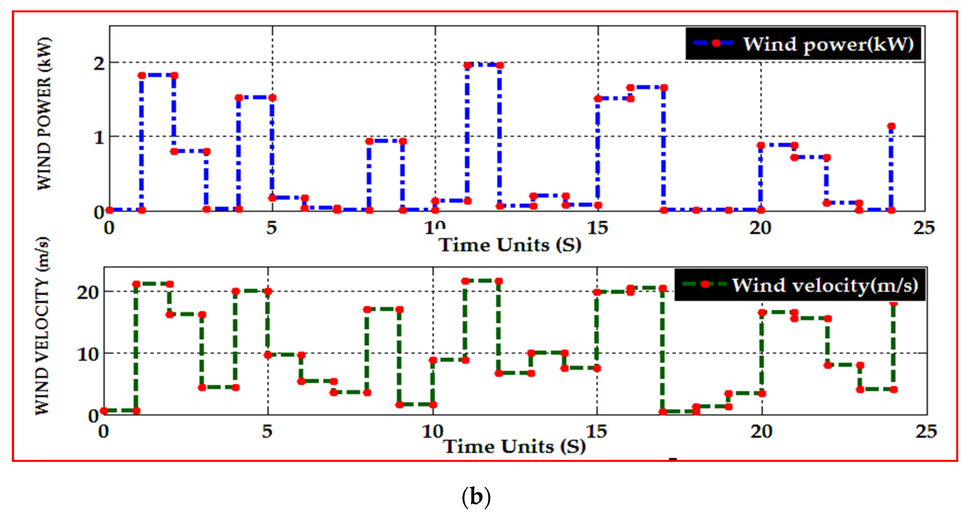
2.1. Design of Virtual VAWT Model

In recent times, VAWTs have becomes more attractive due to its diverse advantages over the HAWT configuration [12,22,34]. The optimum number of blades for a straight-bladed H-type VAWT is three, with a low aspect ratio (height = 0.6 to radius = 0.8 m) that should be less than one. Therefore, Simulink models are constructed for the proposed work by considering these advantages that affect the effective operation of the VAWT model [35,36]. Also, other important factors like the tip speed ratio (TSR) and the power coefficient (Cp) are calculated using a separate subsystem model.
The VAWT model is constructed using wind power Equations (1)–(3) given below and the complete virtual Simulink model, shown in Figure 3a, comprises five sections designated as wind area calculation, turbine speed calculation, power coefficient (Cp) calculating subsystem, and energy calculation unit [37].
In this model, optimum TSR values in the ranges of 0.3 to 2.5 are considered to study the virtual model performance because a better power coefficient exists for the least values [38,39]. The proposed Simulink model accepts the wind speed inputs from 0 m/s to 24 m/s to provide power output from 0 kW to 2 kW, respectively i.e., 0 m/s wind speed velocity is adopted to study the momentary no wind speed effect on total energy generation. Practically, the VAWT model works between cut-in speeds from 2–3 m/s and a maximum cut-out speed of 24 m/s [15,16]. As Per Equation (1), the area occupied by the rotor in contact with the wind flow is proportional to the output power. For a particular area with a selected number of blades, the output is calculated for different wind speeds. The output power is obtained only for the wind speed variations by holding all other values constants in Equation (1).
The simulated power output of the virtual VAWT model and the variation of wind power (kW) output for the random input wind velocity variations from 0 m/s to 24 m/s are given in Figure 3b.
P m = C p ( λ , β ) ρ A V 3   ( W )   where ,   P m = Mechanical   output   power   of   the   turbine   ( W ) C p = P o w e r   C o e f f i c i e n t = R o t o r   p o w e r P o w e r   i n   t h e   w i n d = P m 0.5 ρ ( D H ) V 3 λ = T i p   S p e e d   R a t i o β = B l a d e   p i t c h   a n g l e   ( deg ) ρ = A i r   d e n s i t y   ( kg / m 3 ) = 1.23 A = D H = T u r b i n e   s w e p t   a r e a   ( m 2 ) D = D i a m e t r   o f   t h e V A W T   ( m ) H = H e i g h t   o f   t u r b i n e   ( m ) V = W i n d   s p e e d   ( m / s )
Mechanical   power   ( P m )   normalized   in   p . u P m p u = k p C p p u V 3 P m p u = mechanical   power   ( turbine   power )   in   p . u   for   the   particular   values   of   ρ   and   A
T u r b i n e   s p e e d   ( rpm ) = λ V 60 2 π R   where ,   R = R a d i u s   o f   t h e   w i n d   t u r b i n e   ( m )
Notably, this model is designed to give a maximum power output of 2 kW at 24 m/s cut out speed and it appears at the 11th-time unit and 0 kW at 0 m/s wind velocity is adopted and shown five times in the simulation to study the momentary no wind speed effect on total wind energy generation for 24-time units simulation. Notably, this model is designed to give maximum output power of 2 kW at 24 m/s cut out speed.

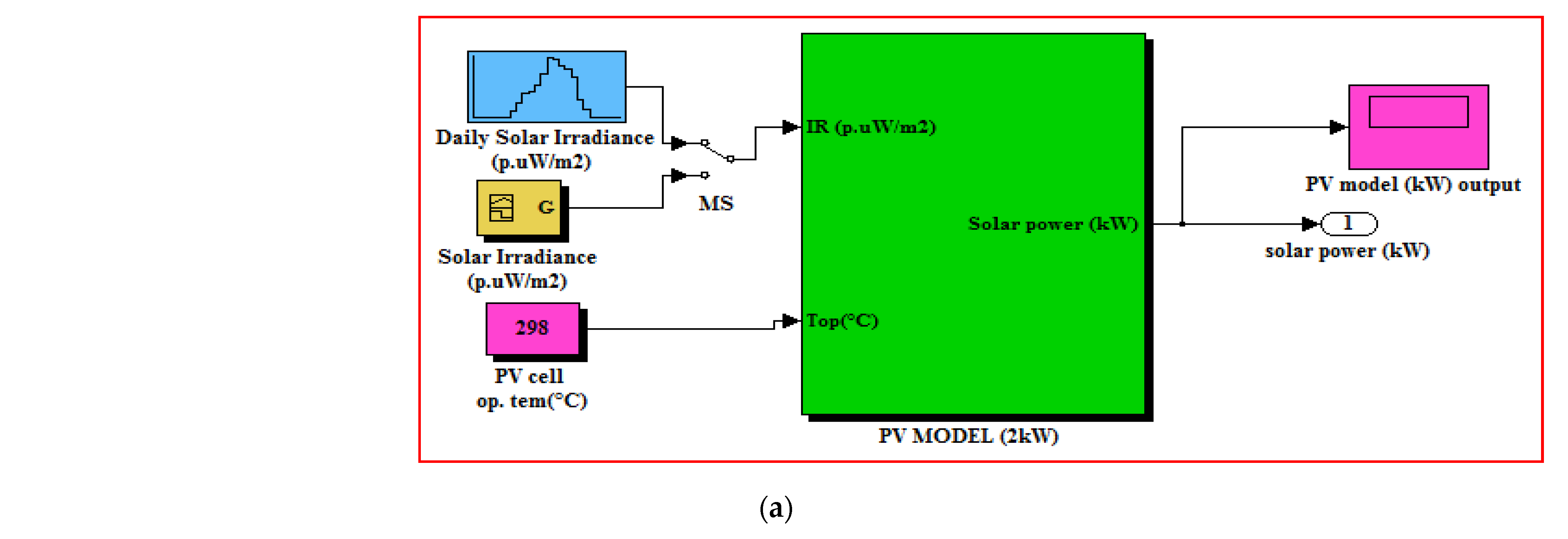
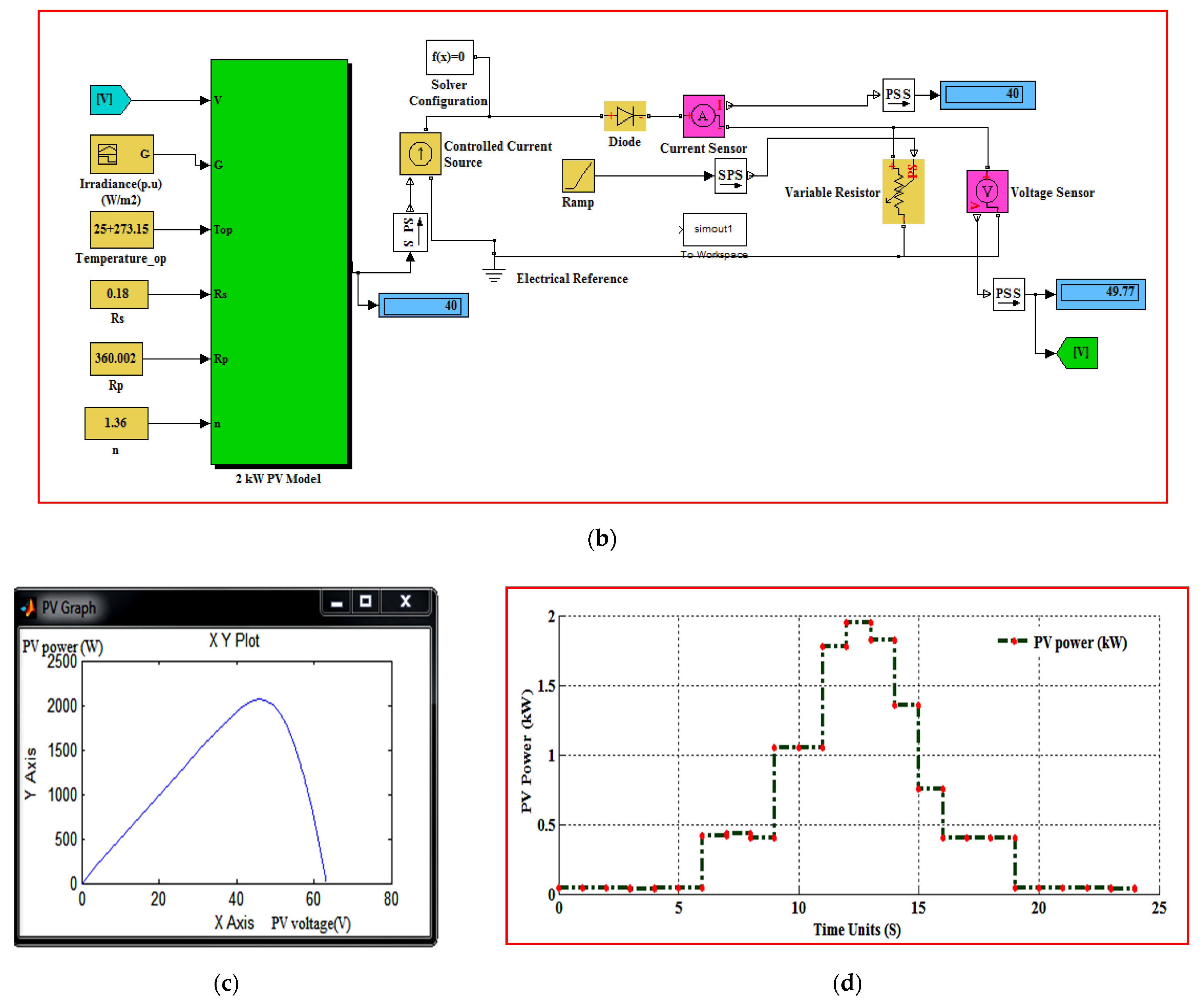
2.2. Design of Virtual PV Module

Energy production using the PV system is the best alternative renewable source for domestic consumers in high solar potential countries like India. Researchers have applied ample efforts to increase the PV module conversion efficiency from 18% to 23% and also progressively reduce the panel cost in the market every year [40]. Attesting to all these factors, the basic PV model in the Simulink environment is shown in Figure 4a and the various internal controllers with their combinations are illustrated in Figure 4b. This PV model is constructed using Equations (4)–(11) for a 60 W Solarex MSX60 PV panel as given below [41]. Further this 60 W PV panel is converted to changing its [NS = 3] series and [NP = 13] parallel connection for the adjustment in PV voltage [51.3 V] and current [45.5 A] (Figure 4c), respectively, to get an approximately 2 kW PV model.
V t = K T o p q w h e r e   V t = Thermal   Voltage   ( V ) K = Boltzmann   constant   1 . 38 × 10 23 T o p = Cell   operating   temperature   in   ° C
q = Electron   Charge   constant   1.6 × 10 19 C V o c = V t ln [ I p h I s ] w h e r e   V o c = Open   circuit   voltage   ( V ) I p h = phase   current   ( A ) I s = Diode   reversed   saturation   current   ( A )
I s = I r s [ T o p T r e f ] 3 e [ q 2 E g n K ( 1 T o p 1 T r e f ) ]
w h e r e   I r s = Diode   reversed   saturation   current   at   Top T r e f = Cell   temperature   at   25 ° C n = Diode   ideality   factor ,   1.36 E g = Band - gap   energy   of   the   cell ,   1.12   eV I p h = G k [ I s c + K I ( T o p T r e f ) ] G k = solar   irradiance   ratio , I s c = Short   circuit   current   ( A )
I = I p h N p I d I s h I = Output   current   from   the   PV   panel   ( A ) N s , N p = No   of   PV   panel   in   series   &   parallel I s h = Shunt   current   ( A )
I s h = [ V + I R s R p ]   R p , R s = Parallel   and   series   resistance   ( Ω )
I r s = I s c [ e ( V o c . q K C T o p . n ) 1 ]
I d = [ e ( V + I R s n V t C N s 1 ) ] [ I s . N p ) ] I d = Diode   current   ( A ) C = No   of   cells   in   a   PV   panel ,   36 STC :   Standard   Test   Condition ,   G = 1   kW / m 2   at   spectral   distribution   of   AM = 1.5   T o p = 25   ° C .
All the above equations are implemented in the Simulink model based on the reference value from a literature survey to obtain the proposed objective. The values of, Tref, Rs, and Rp are considered as 25 °C, 0.18 Ω, and 360 Ω, respectively [42]. Figure 4d illustrates the maximum power output of 2 kW which appears at many samples specifically between 6 to 18-time units based on the solar irradiation profile of the proposed area. Further, the hybrid PV-wind Simulink model is constructed with operating Equations (Equations (1)–(11)), exhibits a good output and may be embedded into a fuzzy logic controller to study the effect of renewable sources on the demand side. The newly designed virtual VAWT and PV model with wind speed variations from 0 m/s (to describe no wind condition) to 24 m/s and the solar module irradiance (G) variation from 250 W/m2 to 1090 W/m2 (0.25 to 1.09 p.u W/m2) [43] are used for effective results. The PV panel output obtained from the simulation model shows the variation rate but exactly matches with the daily solar radiation curve of the selected location [43].

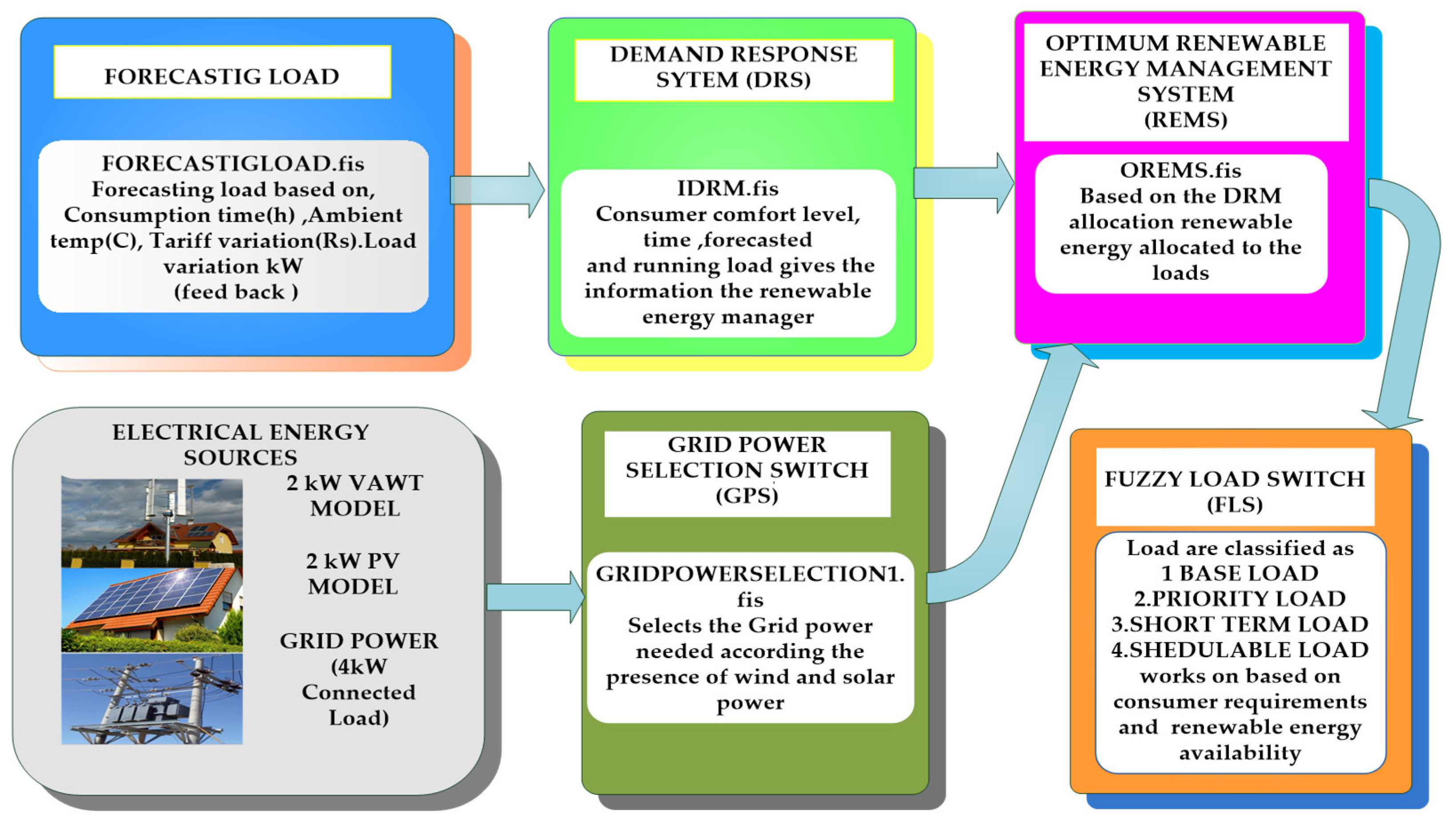
2.3. Proposed Autonomous Fuzzy Controller (AuFuCo)

The architecture of the smart fuzzy logic controller as an autonomous model [44,45] for demand-side management is displayed in Figure 5. This fuzzy controller is designed with the following major components:
  • Virtual Source Model: Wind and PV power resources are designed with their characteristic equations as a virtual model for a rated capacity of 2 kW each and a total capacity of 4 kW. This model is constructed using Simulink and can be easily tunable with input side variations like wind speed and solar irradiance parameters which reflect on the output power.
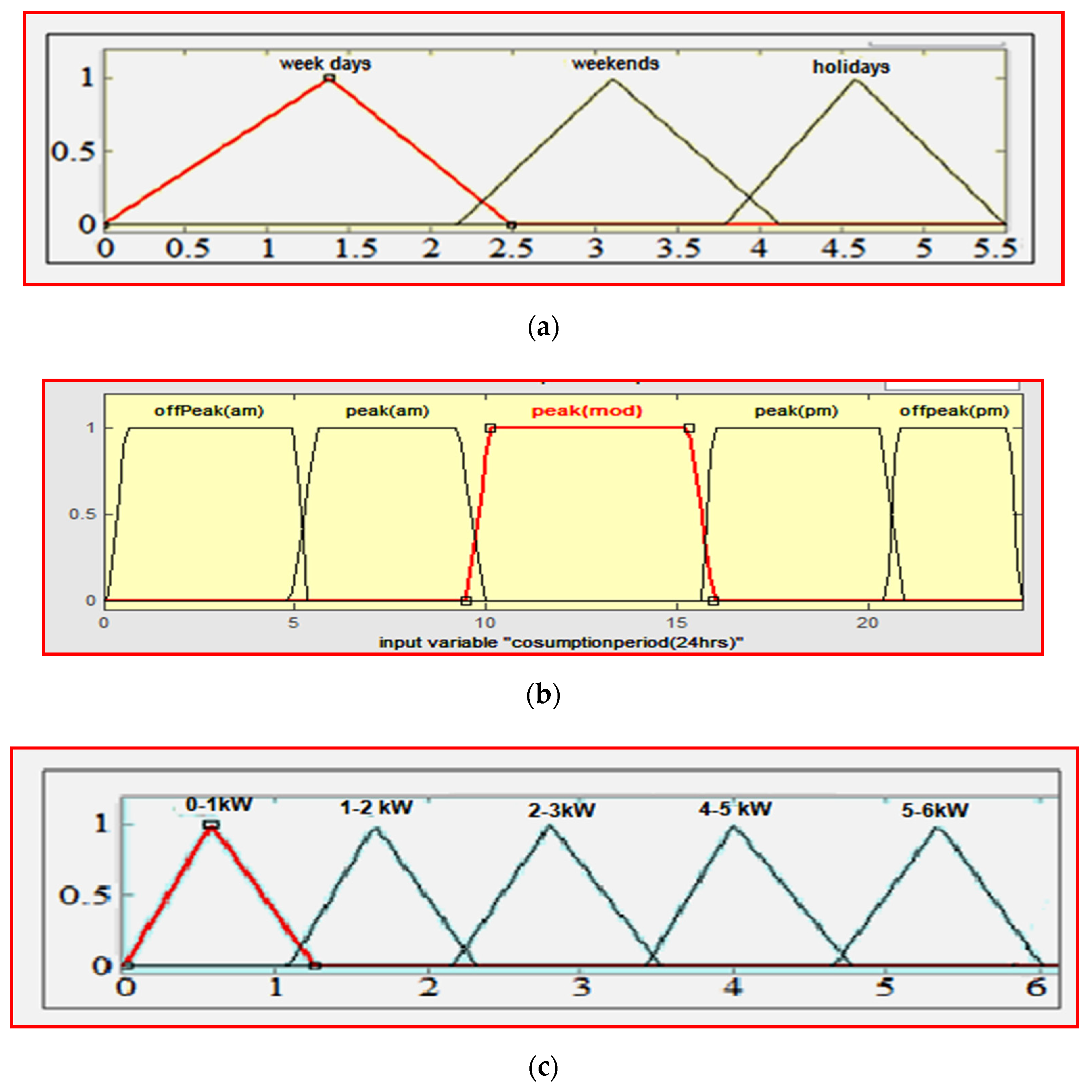
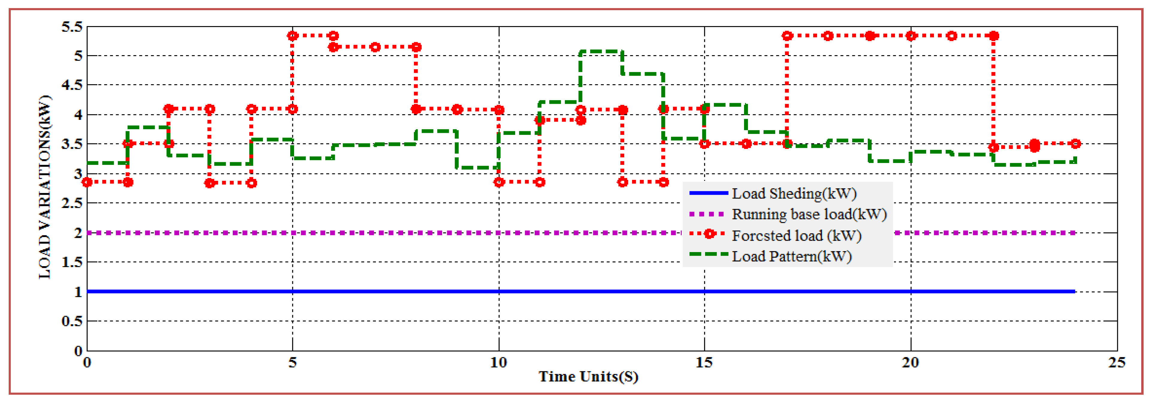
  • Forecasting System (FS): It is constructed with a fuzzy inference system (FIS) for predicting the load demand variations based upon electricity tariff, time of consumption, and ambient temperature.
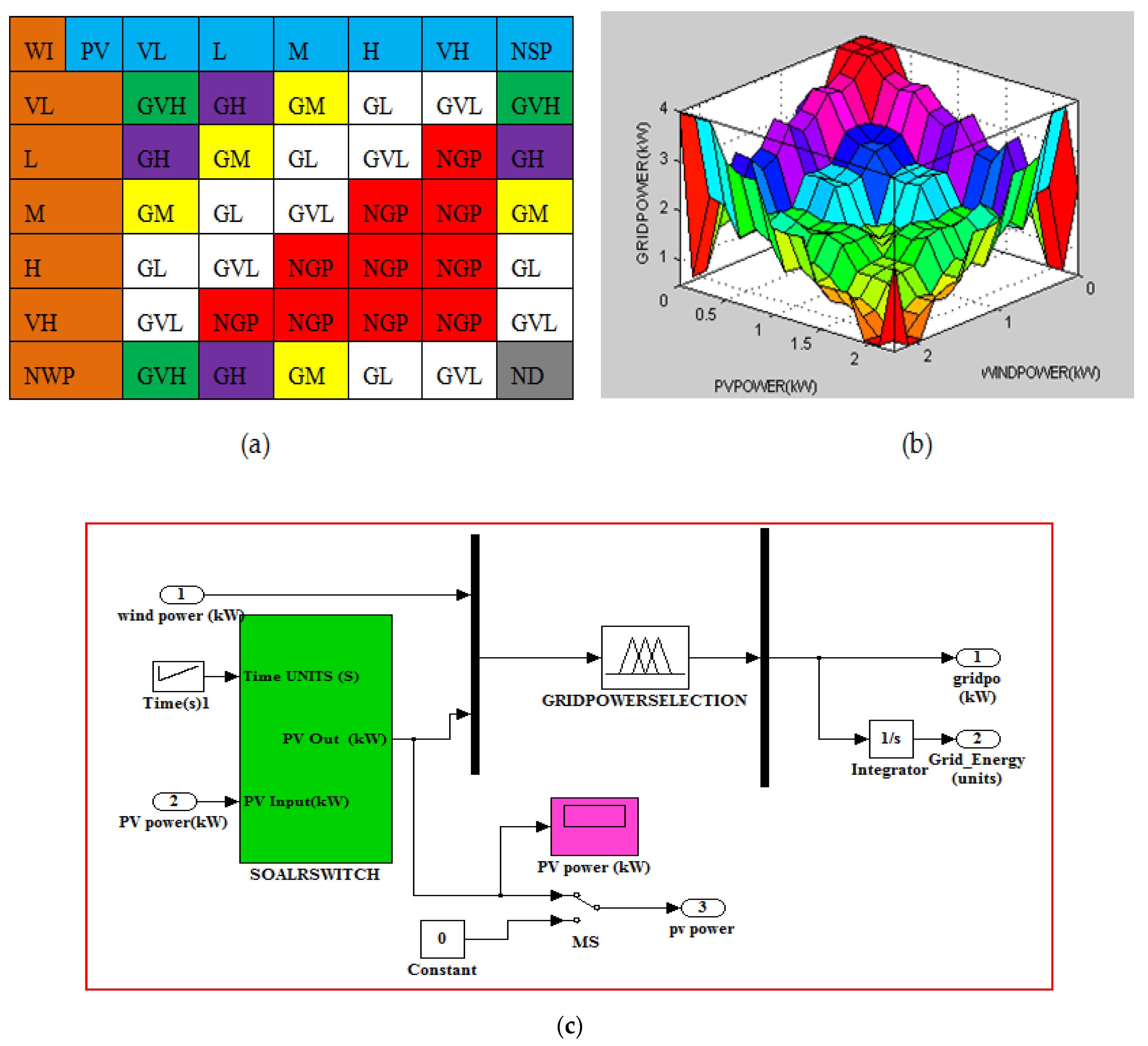
  • Grid Power Selection (GPS) Switch: This component plays an important role in the selection of energy resources for different load conditions at different times and is constructed using a fuzzy inference system. This fuzzy system effectively decides and manages the amount of grid power needed, considering the availability of renewable energy sources on its incidence at all times.
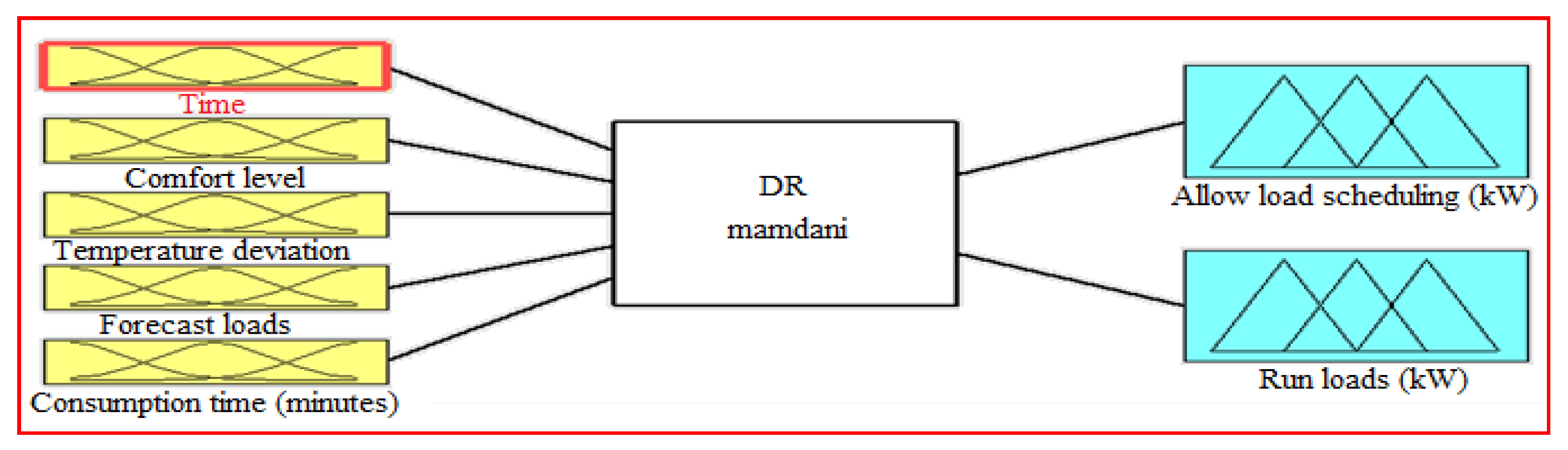
  • Demand Response System (DRS): This unit considers consumption time, comfort level, temperature variations, and energy consumption by sacrificing a little amount of comfort level to calculate the running load in the system.
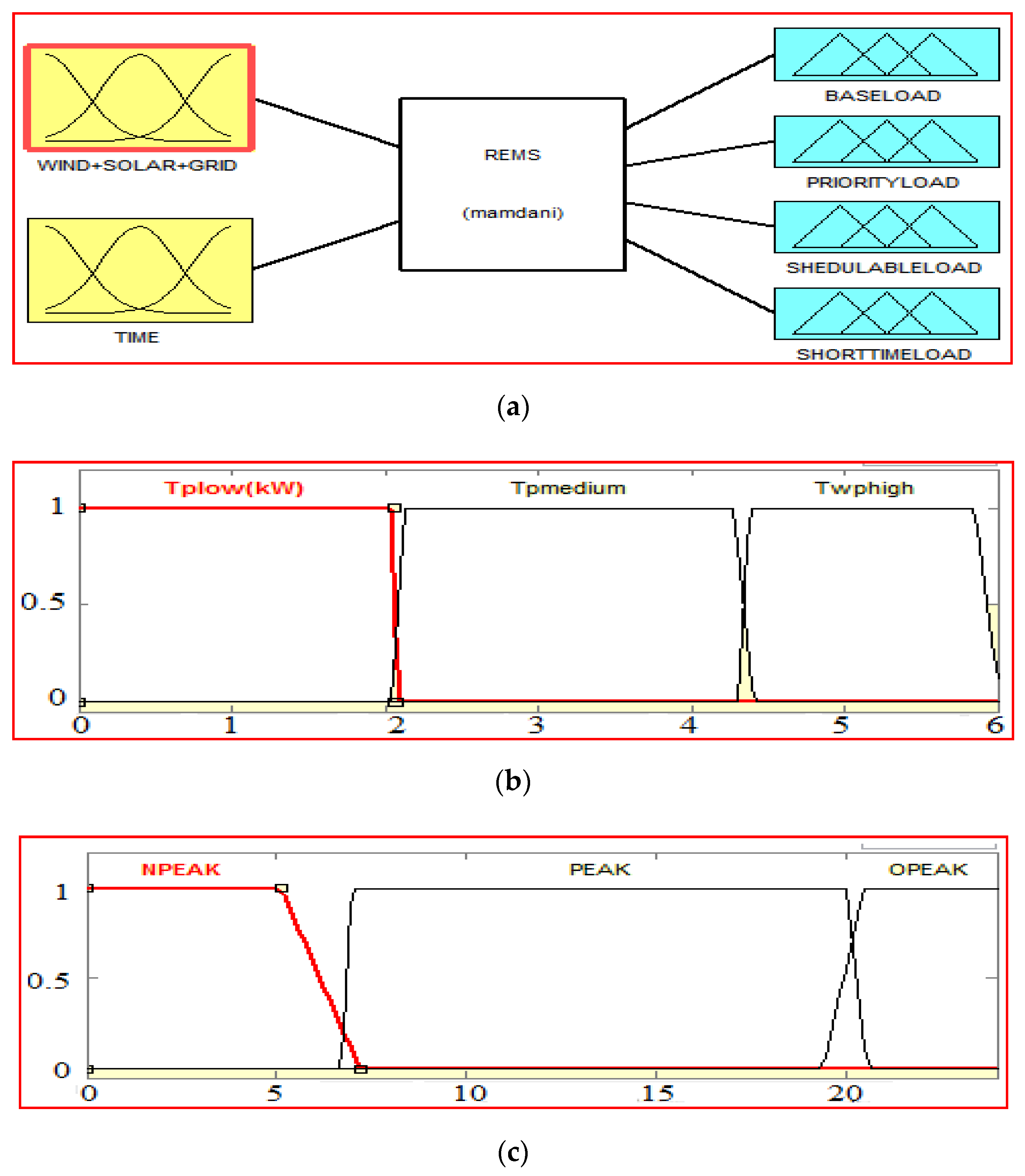
  • REMS: The main purpose of this system is to supply as much renewable energy to different categories of loads available on the domestic consumption side.
  • Fuzzy Load Switch (FLS): This is an intelligent power switch, which enables us to classify different loads to consume power according to the availability of renewable energy sources on the generation side. The loads are classified into four important categories to illustrate the renewable energy impact on demand-side management [40].
    Baseline load: It may be activated at any time or maybe in standby mode to consume the electricity. Example: TV, fan, refrigerator, computer and lighting loads.
    Priority load: It may consume power for a longer time but it can be interrupted for modifying the consumption pattern. Example: air conditioners, heating, and ventilation systems.
    Burst or short term loading: Appliances that consume energy in a single stretch called burst loads. Example: mixers and other cooking appliances
    Schedulable load: Appliances that consume power in a flexible mode. Example: washing machines, wet grinders or pump motors.

3. Methodology

This section describes a smart fuzzy controller using a fuzzy interface system. The fuzzy logic method facilitates the studies for heating, ventilation, and air conditioning (HVAC) demands response systems [46].

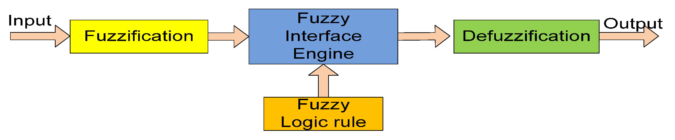
3.1. Introduction to Fuzzy System

The fuzzy logic system uses fuzzy variables for computing its output called inference. All real-valued input data is first fuzzified with membership functions. A membership function assigns a truth value between 0 and 1 to each point in the fuzzy set’s domain. There are four steps used to execute the fuzzy system (1) Fuzzification of input variables (2) rule evaluation, (3) aggregation of the rule outputs and (4) defuzzification, which are illustrated in Figure 6. The rule-based system represents the knowledge of the outside world and specifies how to react to input signals as well. It consists of several simple IF-THEN rules and the controller design proposes the Mamdani-type rules because they provide a natural framework to include expert knowledge in the form of linguistic rules which act as major importance in this problem.
The centre of gravity (COG) approach is used for defuzzification:
COG = i = 1 m μ A ( x ) . x i = 1 m μ A ( x )
where μA is the membership function of the fuzzy set A, x is the elements of the membership function in the universe of discourse and m is the number of rules applied to the controller.

3.2. Fuzzy Inference Systems Used in the Controller

The proposed smart fuzzy logic controller (SFLC) executes output through four major fuzzy inference systems. They are: (1) forecasting system (FS), (2) grid power selection (GPS) switch, (3) renewable energy management system (REMS) and (4) fuzzy load switch (FLS). These fuzzy inference systems are connected with the hybrid wind-solar virtual energy resources and perform the control actions as per the fuzzy rules framed with the real-time input variables.

3.2.1. Forecasting System (FS)

The FS consists of four important variables like consumption time, ambient temperature, tariff variation, and daily load variations [47,48] as shown in Figure 7a–c. The energy consumption variations are recorded on weekdays (normal days), holidays, and weekends and therefore another variable added as a load variation on the fuzzy input side as shown in Figure 7a. The consumption time considers peak and off-peak timings of load in 24-time units (hour) format because the variation of peak demand from 7:00 a.m. to noon and 6:00 to 9:00 p.m. is dominant in the system load consumption as shown in Figure 7b and forecasted load output variation of from 0–6 kW obtained through the fuzzy rules that framed using fuzzy inference system as shown in Figure 7c. The domestic load variations take the upper hand because of the temperature variations and therefore the ambient temperature is also considered in forecasting load. The tariff variations are included to study the cost effect on the load side for investigating demand-side effects on energy cost. The fuzzy forecasting system Simulink model output presented in Figure 8 and also shows that the forecasted load peak exists for domestic consumers are predicted by the FS and managed through a proper allocation load to consume power (running load) or a minimum amount load shedding if it exceeds more than the allocated power at that point of time and all these output information goes to demand response manager. The base load requires the power at any time so that the FS allocates 2 kW.

3.2.2. Grid Power Selection (GPS) Switch

The grid power selection switch collects the input from the virtual hybrid model to the rated capacity of 4 kW, which is simulated for wind speed and solar irradiation variations. The switch proficiently takes the requirement of grid power from the supply mains. These PV and wind power fuzzy variables are classified as very low (VL), low (L), high (H), medium (M), and very high (VH) with 0.4 kW power variations for smooth transitions as shown in Figure 9a,b. Similarly, the output variables are defined using similar classifications at 4 kW with 0.8 kW power variations and are within the variables as shown in Figure 9c.
There are 24 IF-THEN rules framed to collect the right grid output from the supply mains and the rules describe that whenever the wind and solar power remain high there is no necessity for collecting power from the grid mains as shown in Figure 10a. The GPS fuzzy surfaces are shown in Figure 10b explain how this GPS inference system effectively manages the grid power supply from no renewable power duration to maximum renewable power to optimize the usage of hybrid energy on its incidence. GPS collects input energy from the virtual VAWT and PV model for its random wind and irradiance variation and then according to the defined fuzzy rules in GPS decides the amount of power that needs to be fetched from the grid at the given time. The grid power taken is then integrated to convert it into energy calculation as shown in Figure 10c. Silmilarly the wind and PV power supplied also converted in the energy and taken for the energy cost calculation by multiplying its energy cost market prices in $/kWh.

3.2.3. Renewable Energy Management System (REMS)

The REM system collects input from the grid power selection switch and also renewable power added together as another input variable. This input consists of three variables to define total power variations as Tplow, Tpmedium, Tphigh in kW as shown in Figure 11a,b. The other input, variable consumption time, is classified as no peak(NPEAK), peak and off-peak timings (OPEAK) and these are used in REM as shown in Figure 11c and based upon on these two input variables the REM allocates the power to the classified loads according to the requirements of energy consumption. The demand response system considers five input variables as displayed in Figure 12. And the fuzzy variables are named time, comfort level, forecasted load, and temperature deviation and consumption duration. DR based on the fuzzy rules selects the permitted running load and approved load shedding if the load exceeds more than the connected load is given to REM. The load consumption for baseline load is kept ON as illustrated in Figure 13 because this load may be switched ON at any time or kept at standby mode. Therefore, a load of 1 kW is allocated at a time, except for the priority load (1.2 kW).

3.2.4. Fuzzy Load Switch (FLS)

The connected load for domestic consumers is fixed at 4 kW. The fuzzy load switch collects all output of the renewable energy management (REM) system and also collects the output of the wind and the solar energy from the virtual models to allocate power for the schedulable loads. The adapted loads are allowed to consume power whenever the renewable energy generation is in high mode. In this switch, every classification of loads enables its consumption based upon its fuzzy inference system. The base load gathers the inputs from REM and running load output, and tries to keep them alive for all the 24-time units. In priority loads, either air conditioning loads or any other type of room heating appliances are allowed to consume power from available energy resources. Similarly, the short term loads look in the presence of priority load consumptions to allocate power for the short term loadings. The four classified loads are allowed to consume power according to the description as shown in Figure 13. It shows that the base load need turned on at any time in a day and hence FS allocates its power The short term and schedulable load consume a small amount of energy. The schedulable allowed consuming it energy during maximum renewable power availability. All four types of load are allowed to consume 96 units of energy for 24 units of the period, which means that each type of load is allowed to consume 24 units of energy. Figure 14 shows the membership functions of schedulable loads in which the pump motor and the washing machines are allotted to consume power whenever the renewable energy available is high from the source side. All four classified types of loads are allowed to consume a maximum of 1 kW with enabling control from the FLS. In this analysis, the renewable power capacity for wind and solar are assumed to combine at a maximum of 4 kW, and the maximum grid supply is restricted to the domestic consumer with 4 kW to meet their connected load capacity. The simulation was carried out for 24-time units (i.e., 24 × 4 = 96 units) of electrical energy, necessary for supplying all types of loads at any time. To supply this energy, the grid power switch controls the output to satisfy the load energy requirements. The grid power selection switch always looks at the presence of renewable energy for supplying the required load. If this energy level is less or not available, then it allows the grid power to be provided accordingly from grid mains.

4. Results and Discussion

A case study is carried out on this proposed autonomous fuzzy controller (AuFuCo) to optimize the renewable handling on the domestic side. Some assumptions and the list of input values for simulation are given in Table 2. A detailed description of loads from a domestic consumer is listed in Table 3. The assumptions are as follows:
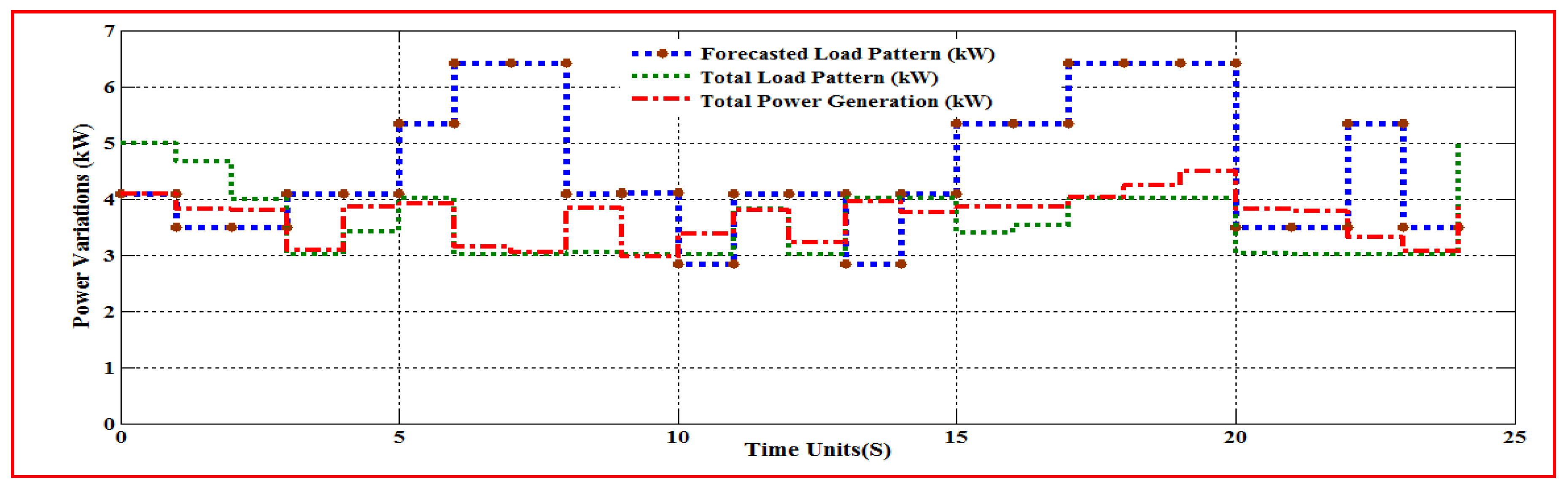
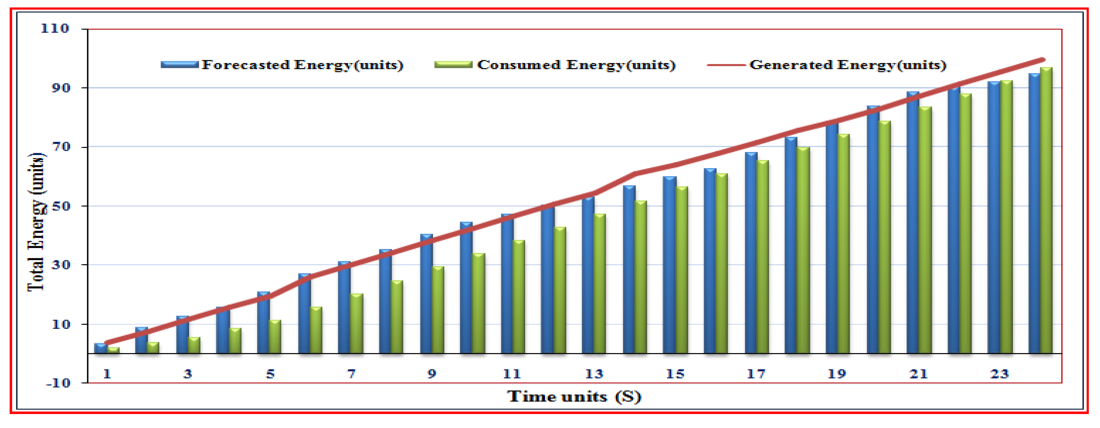
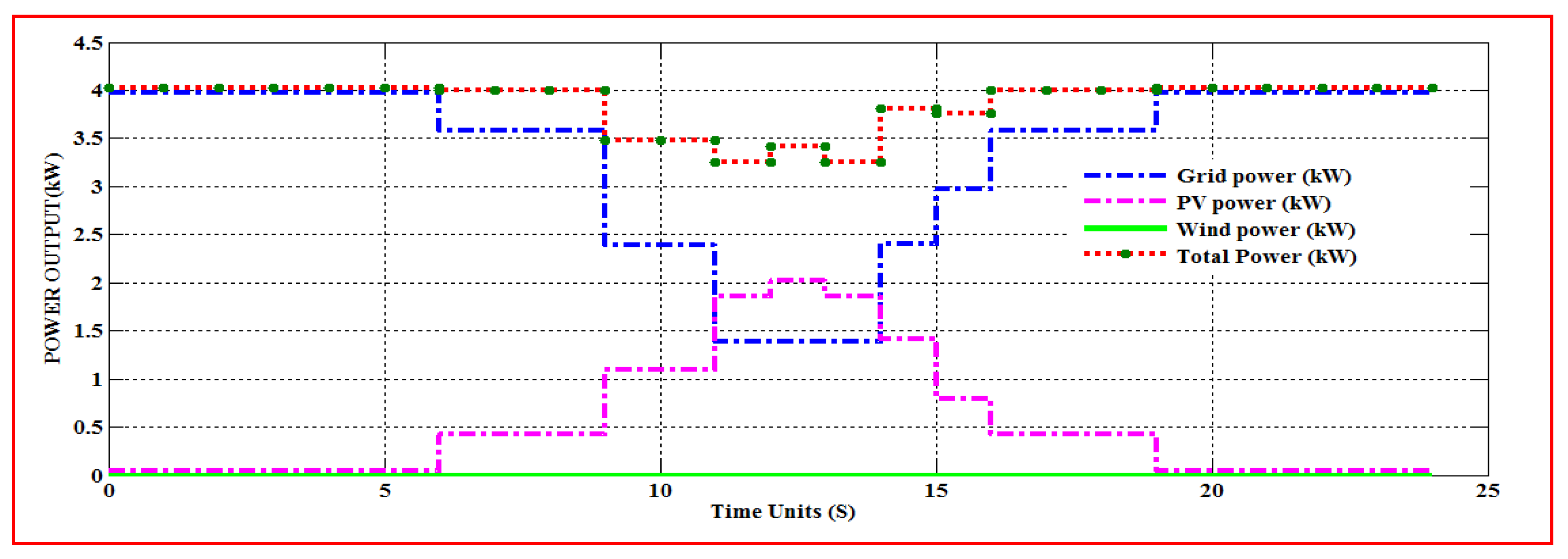
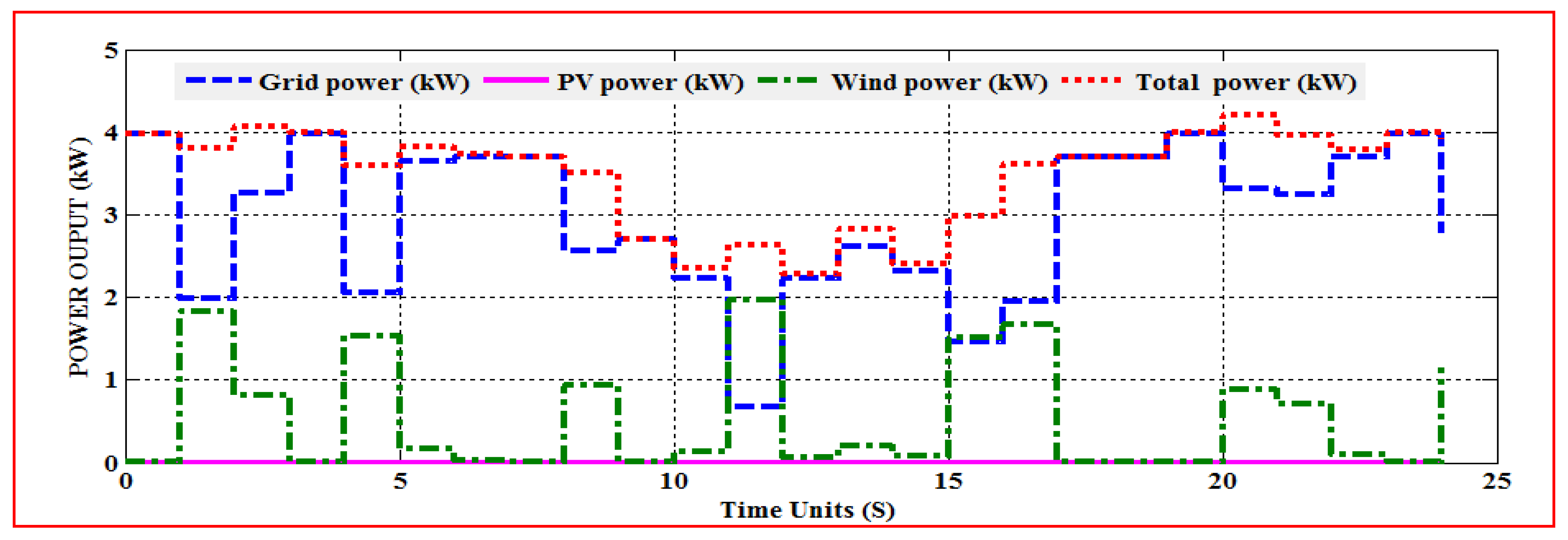
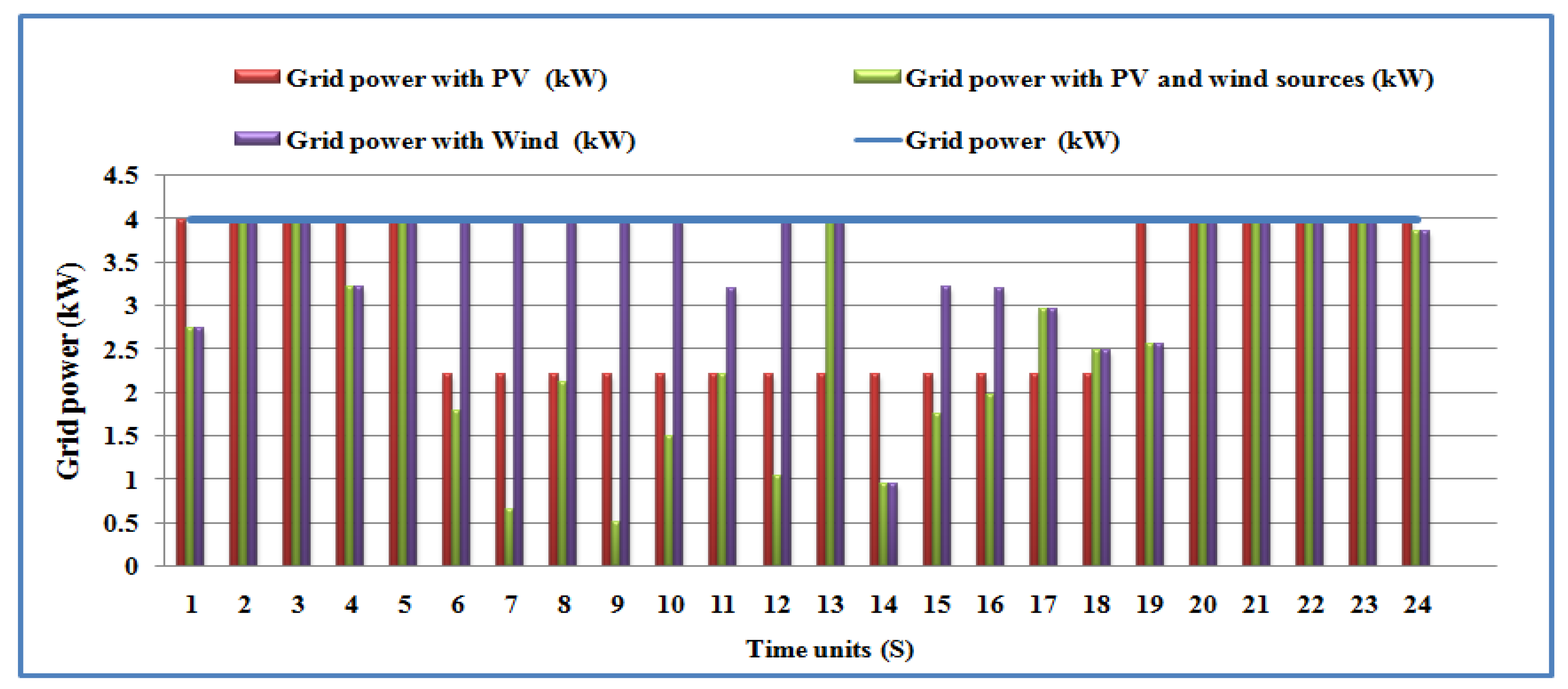
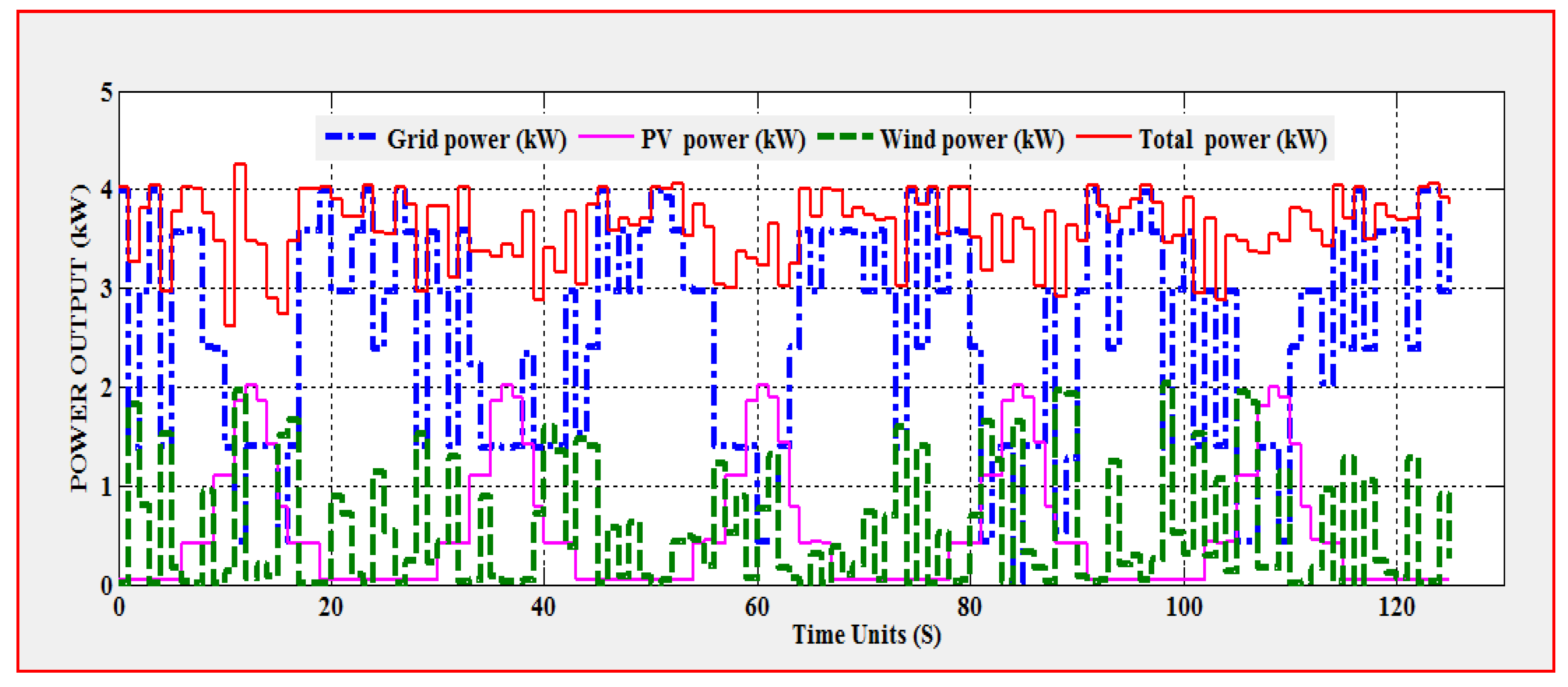
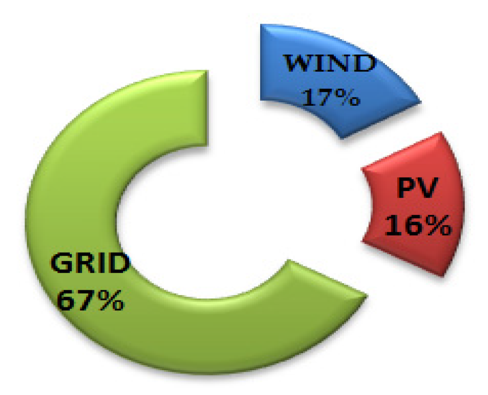
  • The main goal of this analysis is to utilize the hybrid wind and solar energy on its incidence (any time in 24 h) for the maximum possible connected load with grid support through a proposed autonomous (mode) controller and aims to reduce the dependency on the grid.
  • This work is carried out without battery storage support with a high-efficiency inverter configuration (98% percentage of efficiency) but its effect is not considered for output results.
  • Hybrid energy resources are capable of delivering a rated power to a 4 kW connected load.
  • To reduce the peak demand on the grid, a schedulable load is proposed and it consumes energy in the presence of maximum renewable energy incidences.
In this work, all the classification of loads is allowed to consume maximum power of 1 kW at any time by obtaining control from FLS. In this process, the generated energy and its cost on load consumption of 96 Units of energy (4 kW for 24-time units) with the different combinations of energy resources are recognized such as (1) PV with grid supply, (2) wind with grid supply (3) PV, wind, and grid supply and (4) grid supply. These modes are tested to identify the most favourable renewable source which can be adapted for the demand side management techniques. Further, the energy efficiency of the renewable is varied to see the impact of energy availability (total no. of units) on the consumption side. Also, the progress made in the wind and solar power efficiencies with a considerable reduction in energy cost encourages finding the energy cost effect on these hybrid resources by 2030. In a nutshell, this work focuses one to analyse significant factors like the incidence of renewable sources, energy efficiency, the energy cost variations, the future trend in renewable usage on the domestic side using the proposed z.

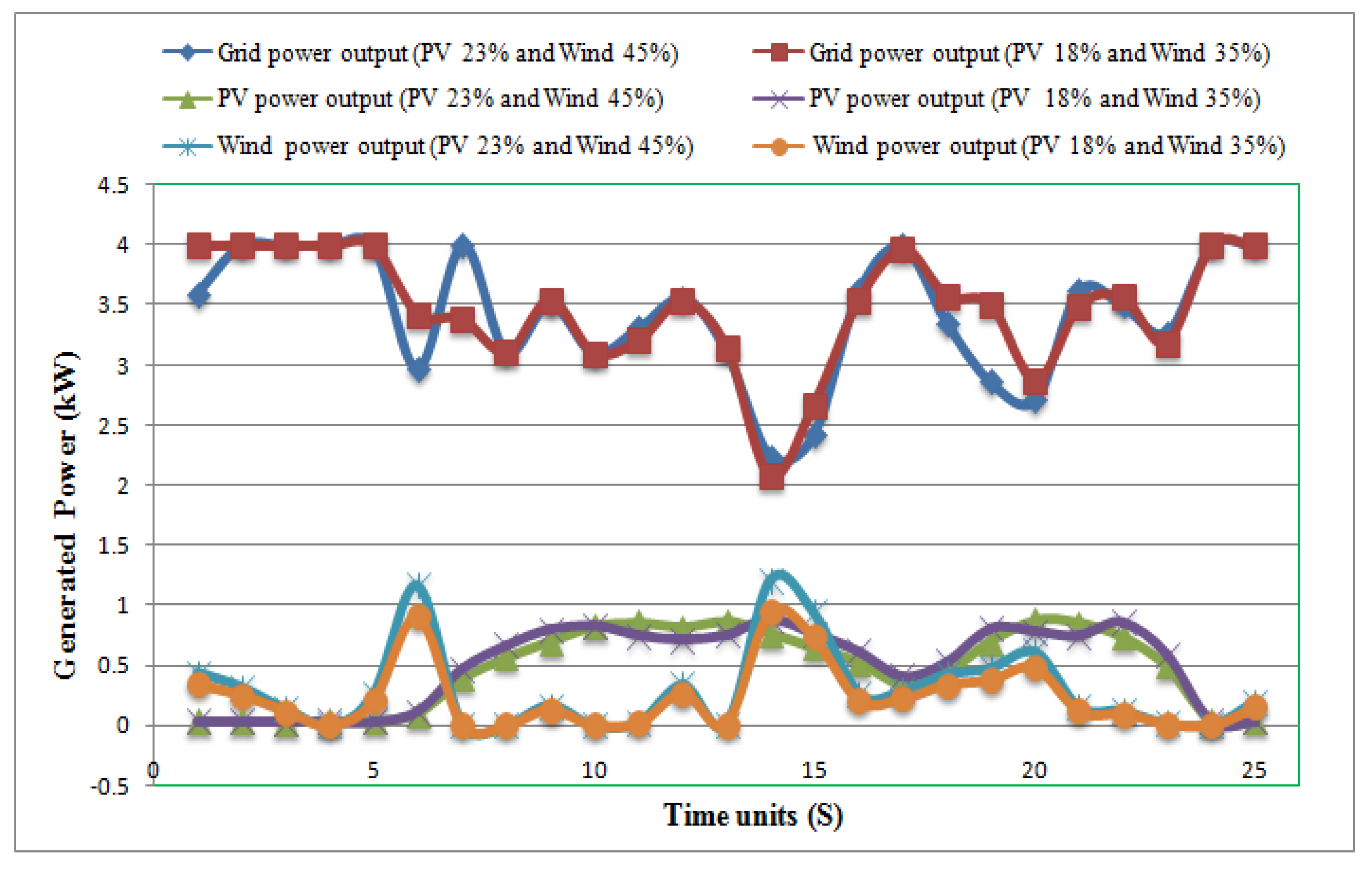
4.1. Analysis of Different Combinations of Hybrid Renewable Energy with Grid Supply

A complete model is designed to meet the total energy and energy cost requirement (Equations (13) and (15)) of the residential consumer loads (listed in Table 2) at any time units with this proposed fuzzy controller (AuFuCo). This analysis focuses to minimize the total grid energy cost of a domestic consumer using Equation (13) subjected to the energy balance constraints as represented in Equation (14). This constraint illustrates several combinations of sources such as grid, PV and wind resources that should meet the demand at any time (t) as per the domestic load requirements. Further, the total energy cost is computed using Equation (15). Notably, the energy supplied by the PV and wind resources is considered to have a negative sign because they are supplied from the domestic side to minimize the total grid energy cost.
Minimize   the   Total   Energy   cost   ( E t cos t ) = t = 1 T ( T O E p r i c e , t × E g r i d , t )   where   T O E p r i c e , t = Energy   cost ( Rs / kWh ) at   time   t   ( hours ) E g r i d , t = Energy   supplied   by   the   grid   ( kWh ( or ) units )   at   time   t   ( hours ) Subjected   to   energy   balance   condition ,
( E g r i d , t + E   P V , t + E w i n d , t ) = E t D     Where ,   t = 1 , 2 , T ( t i m e   u n i t s ) E t R = Energy   request   by   the   consumer   at   time   t   ( hours )
Total   Energy   cos t   ( E t cos t ) / day = t = 1 24 [ ( t a r i f f   f i x e d   p e r   u n i t × E g r i d , t ( t ) ) ( P V   cos t   p e r   u n i t × E P V , t ( t ) ) ( W i n d   cos t   p e r   u n i t × E w i n d , t ( t ) ) ] E P V , t ( t ) = Energy   supplied   by   the   PV   panel   ( kWh ( or ) units )   at   time   t   ( hours ) E w i n d , t ( t ) = Energy   supplied   by   the   wind   VAWT   model   ( kWh ( or ) units )   at   time   t   ( hours )  
The virtual model used in the Simulink environment kept their input values unchanged for all four modes of analysis. The H-type VAWT model assumes the wind velocity varies between 0 m/s to 24 m/s which includes both cut-in speed of 2 m/s and cut-out speed of 24 m/s. The uncertainty in wind availability is simulated to investigate the effect of renewable energy with solar and grid power. Similarly, the solar irradiance (p.uW/m2) variations given in the inputs are between 0.89 to 1.09 [41,49].The unavailability of solar power in the absence of the Sun is also included in this analysis. The wind energy cost (0.036 USD/unit), solar energy cost (0.041 USD/ unit), and average coal energy in the market (as of September 2020, 0.061 USD per unit) is assumed [5] for total energy cost calculations. The Simulink results shown in Figure 15 indicate the energy supply combination of renewable sources with grid supply balanced by the AuFuCocontroller without exceeding 4 kW connected load and these results justify the fetching mode of grid power from the mains when the renewable energy is less or unavailable.
Figure 16 shows the effectiveness of the designed fuzzy controller that balances the forecasted demand and the hybrid renewable generation along with grid support. The controller acquired the forecasted load pattern and effectively manages the peak demand without exceeding the proposed load demand. Figure 17 illustrates the effectiveness of the controller in how it balances the forecasted and generated energy with load energy consumption variations. In addition to this, we verified that the proposed fuzzy controller has the ability to match the load consumption in the absence of wind and PV power along with the grid and it is shown in Figure 18. In this case, the wind power kept at zero levels and the existence of PV power the grid power was fetched from the grid supply and maintains the maximum load at 4 kW. Similarly, Figure 19 illustrates the impact of wind power variation on the grid power supply to meet the 4 kW connected load by keeping the PV power level at zero is also verified with this proposed fuzzy controller.
It is observed that the wind and solar power combination with grid power supply exhibit the least cost (from Equation (15)) to the consumer which is noticeably (16.69%) less than the grid supply. It is also noted that the PV, wind and grid combination provide a net energy savings of 52.81% and a portion of the grid power supply (62.67 kWh) is recorded with the least percentage of 69.63% in PV, wind, and grid combination (Table 4).
This hybrid combination is recommended for domestic applications that allow consumers to load the schedulable demand rate during the off-peak grid period. It is noted in Figure 20 that the peak load forecasted period is shifted with the feasibility in the operation of those schedulable loads. The simulated output of all three combinations with grid supply gives a noticeable result for placement of wind and PV power in the demand side, which supports the demand side management techniques such as Peak shifting and Valley filling [50] as shown in Figure 20. Except for the wind power combination because of its natural wind velocity variation, the other two combinations show peak power consumption (normally happens in the domestic consumption between 9 a.m. to 9 p.m.) shift to the off-peak period. This is an exceptional outcome because of PV power in the generation system with its constant supply of power to the demand side. Therefore, it is concluded that the peak shifting and valley filling PV source of energy generation is preferred extensively over wind power generation. But the presence of wind power throughout the day (even with variations) is considered the best choice of energy source and may be considered as a hybrid system with PV and wind power).

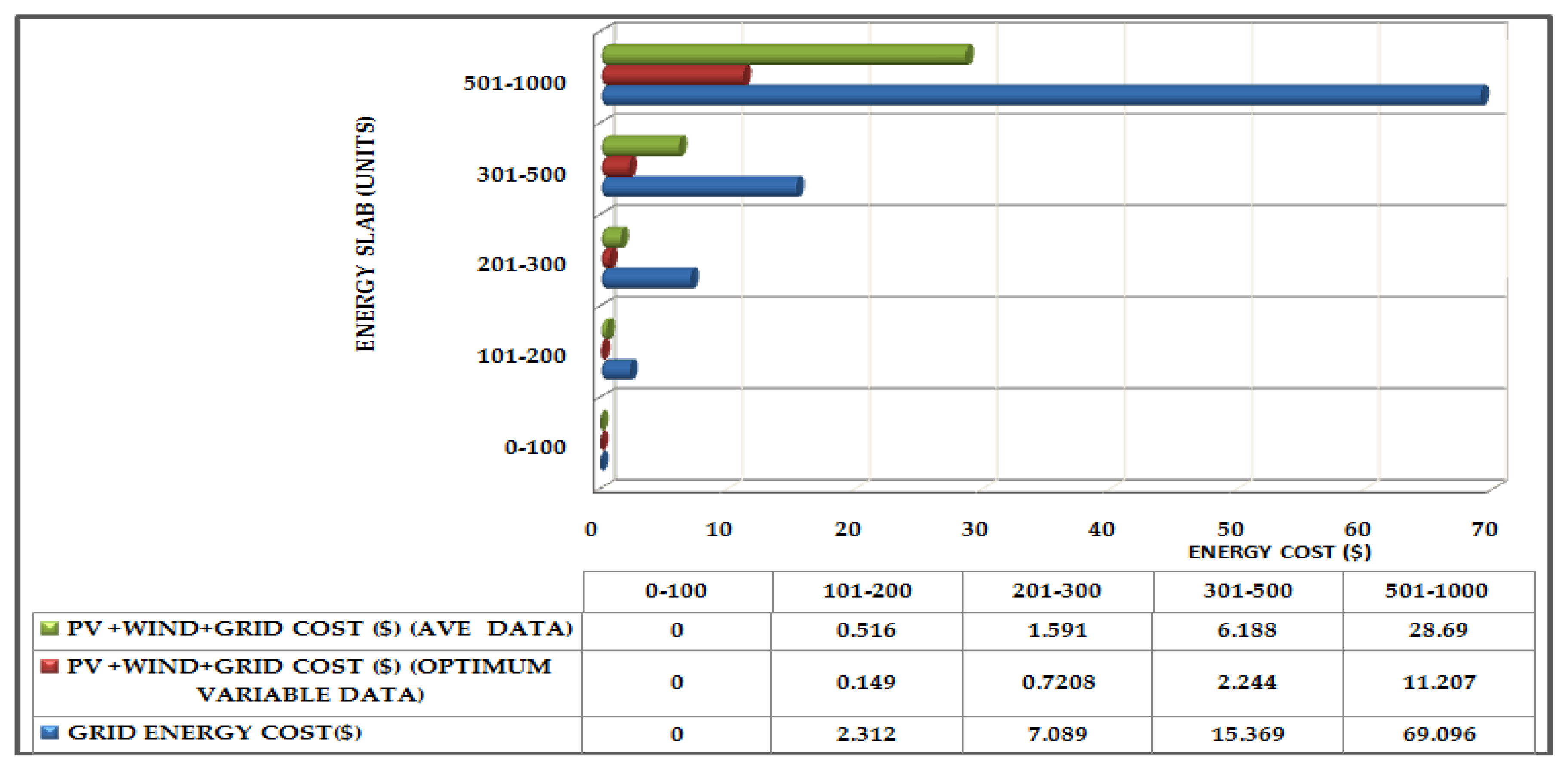
4.2. Analysis of Energy and Cost Savings Based on Home Environment Energy Tariff

Based on the practical local tariff rate of energy, the proposed controller is adapted to evaluate the total energy and cost savings due to the impact of hybrid energy resources with the grid system for a domestic consumer (cost proportional to units consumed). The grid power selection (GPS) switch in the controller has the intelligence to meet the total demand of the consumer based on the presence of PV and Wind renewable energy that is evaluated using Equations (13) and (14). Also, the total energy cost is calculated using Equation (15). As stated earlier, the maximum demand of 4 kW connected load with 24 units is considered for this study that consumes 96 units (kWh) of energy. The electricity tariff slab with corresponding local electricity charges for a domestic consumer is shown in Table 5. In this analysis, simulation is done with 25 units that consume 100 units of electricity. Similarly, run times of 50, 125, and 250 consume 200, 500, and 1000 units respectively. Further, the solar irradiance variations are tuned between 0.4–1.4 p.uW/m2 as optimum data and wind speed is used as a random variable between 0 to 22 m/s. The average irradiance of 0.8 p.uW/m2 and wind speed of 12 m/s is considered to identify the variation between optimum and average renewable energy utilization.
The observed results are shown in Figure 21 for 125-time units for optimum random variable data and the electricity block-based results for optimum and averaged data are tabulated in Table 6. It is observed that there is an inconsistency in wind power compared with solar power generation. Further, Figure 22 demonstrates the participation of all the energy resources in the 1000 units block with optimum data. It is noticed that the wind generation is reduced to the least value of 8% in the case of 10 m/s wind velocity. During good atmospheric conditions, a higher rate of about 60.1% of energy is served by the renewable resources, and the respective energy costs with variations are shown in Figure 23. This cost-based study using hybrid renewable energy resources on the domestic side shows significant cost savings results for consumers. Considering the bi-monthly billing concept, the total cost of energy is about 69.04 USD for grid-based demand management but it is least i.e., 11.20 USD for an optimal data hybrid combination which is 83.77% less compared with grid power cost. The observed results reveal that the total savings of 242.20 USD/year for an average proposed data and 344.35 USD/year for an optimal condition can be accomplished by considering approximate cost function; 750 USD/kW (PV) and 850 USD/kW (VAWT). A total cost savings of 344.35 USD/year can be attained through optimal conditions that can significantly reduce the amortization period by about 8 to 9 years for a domestic consumer. This proposed strategy can be strongly recommended for future expansion of energy demand management and it can act as a potential investment for a domestic consumer toward comfortable energy consumption for more than 25 years without environmental pollution.

4.3. Effect of Energy Conversion on DSM Technique

The effect of energy conversation on the demand side is investigated with this AuFuCo model [39] and it is tested through the increasing single point energy efficiency of wind and PV systems. In the present scenario, solar panels are available at 18% conversion efficiency, and the VAWT model wind turbine available at 35%. This conversion efficiency is increased to 23% and 45% for PV and wind systems respectively. These variations are included in virtual model simulation, which gives similar characteristics of energy conservation of demand-side management techniques. The improved conversion efficiency on PV and VAWT model able to record about (5.76–5.78 USD) 0.5% reduction in energy cost which is least compare with conventional controller (Table 7) and also 1.25% reduction in grid supply. Figure 24 implies that the placement of renewable sources on the demand side improves the source conversion efficiency similar to the energy conservation obtained by increased load efficiency. The above discussed one point source efficiency improvement methods are convincing practice and superior to the multi-points load efficiency practice in DSM technique.

4.4. Effect of Hybridization on Demand-Side by 2030

The motivating outcomes of hybridization specifically are cost reduction and conversion efficiency improvements, which pave the way to reduce the dependency on coal or oil-based energy resources by 2030 [51,52]. In this study, the present energy efficiency and energy cost are included in the simulation by assuming flat capital expenditure (CAPEX) and operational expenditure (OPEX) per kilowatt of solar and wind turbine [53]. The cost of energy is evaluated using the ratio between present value cost (CAPEX and OPEX) and annual energy production with a 40% capacity factor. The rate of CAPEX (7144.76 USD/kW for a wind system and 613.58 USD/kW for PV) and OPEX (231.80 USD/kW for wind system and 272.70 USD/KW for PV) of both installations are considered for the computation of the energy cost. Also, the lifetime of the wind and PV installations are considered to be 25 years.
The improved conversion efficiency of PV panels (25%) and VAWT model (40%) are considered and the energy cost of PV and wind power are assumed about 0.026 USD and 0.031 USD per unit respectively along with the expected coal power energy cost in the energy market of 0.095 USD per unit [8]. The complete analysis of the results is labeled in Table 8.
It is assumed that maintaining the same amount of renewable energy, 30.8% of additional cost need to spend by 2030. Notably, the cost of energy about 6% (39.25–36.59) is reduced optimistically with renewable energy for 24-time unit simulation.
Figure 25 and Figure 26 demonstrate the present and future energy costs for different control algorithms, respectively. From the illustrations, it is observed that the proposed AuFuCo exhibits better characteristics than the conventional controller. Therefore, it is possible to increase the proportion of renewable power participation extensively in the total energy supply in the future. The utility may motivate domestic consumers to enhance the commission of solar panels and wind turbines on the domestic side through government incentives, for a smart grid environment. This proposed demand-side source generation may be the future trend and a vital solution for demand-side management. Further, the authors are interested in extending this essential analysis to facilitate the urban area for multiple domestic consumers with a smart fuzzy neural network controller. Further, this work may be extended to attain more realistic optimization using real time available sources and load patterns that can be demonstrated in future works.

5. Conclusions

The proposed autonomous fuzzy logic controller (AuFuCo) with a virtual hybrid wind-solar model and fuzzy inference system provides effective control for optimum utilization of renewable energy along with grid power supply without storage support. From the results, it is observed that the uncertainties of the renewable sources are effectively balanced with the grid supply using the proposed controller and met the energy demand with the least energy cost due to its predefined energy block of a utility in an urban environment. Moreover, the source combination of PV, wind, and grid supply proposed by the controller concede the least energy cost of about 4.89 USD for 90 units which is the best rate when compared with other combinations. Also, the total cost savings of 242.20 USD/year for an average proposed data and 344.35 USD/year for an optimal condition is achieved. The simulation results revealed that the proposed fuzzy controller properly predicts the forecasted energy cost at a reduced level when compared with an existing controller. It identifies the location of hybrid sources on the demand-side concurrently which improves the peak shifting and valley filling capabilities of demand-side management techniques.
This proposed research work suggests that the application of AuFuCo controller with hybrid renewable energy sources offers a solution to meet future demand growth. Also, this controller on the demand side can present a fundamental solution to reduce the dependence of the high cost and highly polluted coal energy from the grid side. However, the proposed virtual model needs to be implemented in a real-time system through encouraging research and technology advancements to validate its effectiveness on hybrid energy consumption with grid supply by considering all ratings described in the analysis to sustain future energy growth.

Author Contributions

Conceptualization, M.A.; Methodology, M.A.; Software, M.A.; Validation, V.P. and A.J.; Formal Analysis, V.P. and A.A.A.; Data Curation, R.K. and M.H.A.; Writing—Original Draft Preparation M.A. and R.K.; Writing—Review & Editing, S.M. and M.-K.K.; Supervision, M.H.A.; Funding Acquisition, M.-K.K. All authors have read and agreed to the published version of the manuscript.

Funding

This research was supported by the Chung-Ang University Research Grants in 2021. This research was also supported by Basic Science Research Program through the National Research Foundation of Korea (NRF) funded by the Ministry of Education (2020R1A2C1004743). In addition, this research support by the Taif University Researchers Supporting Project number (TURSP-2020/77), Taif University, Taif, Saudi Arabia.

Conflicts of Interest

The authors declare no conflict of interest.

Abbreviations and Symbols

VAWTVertical axis wind turbine
HAWTHorizontal axis wind turbine
PVPhotovoltaic
REMSRenewable energy management system
RERenewable energy
HIHREMHome renewable energy management system
HOMERHybrid Optimization Model for Electric Renewable
HVACHeating, Ventilating and Air conditioning
DRSDemand response system
DSMDemand side management
AuFuCoAutonomous Fuzzy Controller
SFLCSmart Fuzzy Logic Controller
EMSEnergy management system
EPSRElectric power survey report
IEAInternational energy agency
LFLoad forecasting
MASMulti-Agent System
ABCArtificial bee colony
STCStandard test condition
GHGrid power high
GLGrid power low
GMGrid power medium
GPSGrid power selection
GVHGrid power very high
GVLGrid power very low
COGCenter of gravity
Egrid,tEnergy supplied by the grid
EtREnergy request by the consumer at time t
EPV,tEnergy supplied by the PV panel at time t
EtcostTotal energy cost
Ewind,tEnergy supplied by the wind VAWT model at time t
mNumber of rules applied to the controller
NpNo of PV panels in parallel
NsNo of PV panels in series
PmMechanical output power of the turbine
RpParallel resistance
RsSeries resistance
TopCell operating temperature
TrefCell temperature at 25 °C
TOEprice,tEnergy cost at time t
SGDMSSmart Grid Distribution Management System
TERIThe Energy and Resources Institute

References

  1. Elavarasan, R.M.; Selvamanohar, L.; Raju, K.; Vijayaraghavan, R.R.; Subburaj, R.; Nurunnabi, M.; Khan, I.A.; Afridhis, S.; Hariharan, A.; Pugazhendhi, R.; et al. A Holistic Review of the Present and Future Drivers of the Renewable Energy Mix in Maharashtra, State of India. Sustainability 2020, 12, 6596. [Google Scholar] [CrossRef]
  2. Krishnamoorthy, R.; Udhayakumar, K.; Kannadasan, R.; Elavarasan, R.M.; Mihet-Popa, L. An Assessment of Onshore and Offshore Wind Energy Potential in India Using Moth Flame Optimization. Energies 2020, 13, 3063. [Google Scholar]
  3. Yang, J.; Urpelainen, J. The future of India’s coal fired power generation capacity. J. Clean. Prod. 2019, 226, 904–912. [Google Scholar] [CrossRef]
  4. Dubash, N.K.; Khosla, R.; Rao, N.D.; Bhardwaj, A. Corrigendum: India’s energy and emissions future: An interpretive analysis of model scenarios (2018 Environ. Res. Lett. 13 074018). Environ. Res. Lett. 2018, 13, 089501. [Google Scholar] [CrossRef]
  5. Report. Accelerating India’s Transition to Renewables: Results from the ETC India Project. 2017. Available online: https://www.teriin.org/sites/default/files/files/etc-key-messages-summary.pdf (accessed on 12 March 2021).
  6. Guttikunda, S.K.; Jawahar, P. Atmospheric emissions and pollution from the coal-fired thermal power plants in India. Atmos. Environ. 2014, 92, 449–460. [Google Scholar] [CrossRef]
  7. Madhu, S.; Payal, S. A Review of Wind Energy Scenario in India. Int. Res. J. Environ. Sci. 2014, 3, 87–92. [Google Scholar]
  8. Remap 2030 Renewable Energy Prospects for Poland. 2015. Available online: https://www.irena.org/-/media/Files/IRENA/Agency/Publication/2015/IRENA_REmap_Poland_paper_2015_EN.pdf (accessed on 21 March 2021).
  9. Lu, X.; McElroy, M.B. Global Potential for Wind-Generated Electricity. Wind Energy Eng. A Handb. Onshore Offshore Wind Turbines. 2017, 106, 51–73. [Google Scholar]
  10. Venkatesan, C.; Kannadasan, R.; Alsharif, M.H.; Kim, M.-K.; Nebhen, J. A Novel Multiobjective Hybrid Technique for Siting and Sizing of Distributed Generation and Capacitor Banks in Radial Distribution Systems. Sustainability 2021, 13, 3308. [Google Scholar] [CrossRef]
  11. Venkatesan, C.; Kannadasan, R.; Alsharif, M.H.; Kim, M.-K.; Nebhen, J. Assessment and Integration of Renewable. Energy Resources Installations with Reactive Power Compensator in Indian Utility Power System Network. Electronics 2021, 10, 912. [Google Scholar] [CrossRef]
  12. Apelfröjd, S.; Eriksson, S.; Bernhoff, H. A Review of Research on Large Scale Modern Vertical Axis Wind Turbines at Uppsala University. Energies 2016, 9, 570. [Google Scholar] [CrossRef] [Green Version]
  13. Niranjana, S.J. Power Generation by Vertical Axis Wind Turbine. Int. J. Emerg. Res. Manag. Technol. 2015, 2, 1–7. [Google Scholar]
  14. Chong, W.T.; Fazlizan, A.; Poh, S.C.; Pan, K.C.; Hew, W.P.; Hsiao, F.B. The design, simulation and testing of an urban vertical axis wind turbine with the omni-direction-guide-vane. Appl. Energy 2013, 112, 601–609. [Google Scholar] [CrossRef]
  15. Anthony, M.; Prasad, V.; Raju, K.; Alsharif, M.H.; Geem, Z.W.; Hong, J. Design of Rotor Blades for Vertical Axis Wind Turbine with Wind Flow Modifier for Low Wind Profile Areas. Sustainability 2020, 12, 8050. [Google Scholar] [CrossRef]
  16. Mohanasundaram, A.; Valsalal, P. Analysis and Design of a Giromill Type Vertical Axis Wind Turbine for a Low Wind ProfileUrbanArea. J. Electr. Eng. 2020, 20, 363–375. [Google Scholar]
  17. The Future of Cooling, Opportunities for Energy-Efficient Air Conditioning. 2018. Available online: https://www.iea.org/reports/the-future-of-cooling (accessed on 12 March 2021).
  18. Xu, L.; Wang, Z.; Liu, Y.; Xing, L. Energy allocation strategy based on fuzzy control considering optimal decision boundaries of standalone hybrid energy systems. J. Clean. Prod. 2021, 279, 123810. [Google Scholar]
  19. Loukil, K.; Abbes, H.; Abid, H.; Abid, M.; Toumi, A. Design and implementation of reconfigurable MPPT fuzzy controller for photovoltaic systems. Ain Shams Eng. J. 2020, 11, 319–328. [Google Scholar] [CrossRef]
  20. Jeong, J.S.; Ramírez-Gómez, Á. Optimizing the location of a biomass plant with a fuzzy-DEcision-MAking Trial and Evaluation Laboratory (F-DEMATEL) and multi-criteria spatial decision assessment for renewable energy management and long-term sustainability. J. Clean. Prod. 2018, 182, 509–520. [Google Scholar] [CrossRef]
  21. Ma, Y.; Li, B. Hybridized Intelligent Home Renewable Energy Management System for Smart Grids. Sustainability 2020, 12, 2117. [Google Scholar] [CrossRef] [Green Version]
  22. Priyadharshini, B.; Ganapathy, V.; Sudhakara, P. An Optimal Model to Meet the Hourly Peak Demands of a Specific Region With Solar, Wind, and Grid Supplies. IEEE Access 2020, 8, 13179–13194. [Google Scholar] [CrossRef]
  23. Deo, R.C.; Ghorbani, M.A.; Samadianfard, S.; Maraseni, T.; Bilgili, M.; Biazar, M. Multi-layer perceptron hybrid model integrated with the firefly optimizer algorithm for windspeed prediction of target site using a limited set of neighboring reference station data. Renew. Energy 2018, 116, 309–323. [Google Scholar] [CrossRef]
  24. Li, W.; Ng, C.; Logenthiran, T.; Phan, V.-T.; Woo, W.L. Smart Grid Distribution Management System (SGDMS) for Optimised Electricity Bills. J. Power Energy Eng. 2018, 6, 49–62. [Google Scholar] [CrossRef] [Green Version]
  25. Tischer, H.; Verbic, G. Towards a smart home energy management system—A dynamic programming approach. In Proceedings of the 2011 IEEE PES Innovative Smart Grid Technologies, Perth, WA, Australia, 13–16 November 2011; pp. 1–7. [Google Scholar]
  26. Zhang, Y.; Zeng, P.; Zang, C. Optimization algorithm for home energy management system based on artificial bee colony in smart grid. In Proceedings of the 2015 IEEE International Conference on Cyber Technology in Automation, Control, and Intelligent Systems (CYBER), Shenyang, China, 8–12 June 2015; pp. 734–740. [Google Scholar]
  27. Shahgoshtasbi, D.; Jamshidi, M.M. A new intelligent neuro-fuzzy paradigm for energy-efficient homes. IEEE Syst. J. 2014, 8, 664–673. [Google Scholar] [CrossRef]
  28. Kushiro, N.; Suzuki, S.; Nakata, M.; Takahara, H.; Inoue, M. Integrated residential gateway controller for home energy management system. IEEE Trans. Consum. Electron. 2003, 49, 629–636. [Google Scholar] [CrossRef]
  29. Gioutsos, D.M.; Blok, K.; van Velzen, L.; Moorman, S. Cost-optimal electricity systems with increasing renewable energy penetration for islands across the globe. Appl. Energy 2018, 226, 437–449. [Google Scholar] [CrossRef]
  30. Bissey, S.; Jacques, S.; le Bunetel, J.C. The fuzzy logic method to efficiently optimize electricity consumption in individual housing. Energies 2017, 10, 1701. [Google Scholar] [CrossRef] [Green Version]
  31. Keshtkar, A. Development of an Adaptive Fuzzy Logic System for Energy Management in Residential Buildings. Thesis Submitt. 2015. Available online: http://summit.sfu.ca/item/16759 (accessed on 26 August 2015).
  32. Rathaiah, M.; Reddy, P.R.K.K.; Sujatha, P. Adaptive Fuzzy Controller Design for Solar and Wind Based Hybrid System. Int. J. Eng. Technol. 2018, 7, 283. [Google Scholar] [CrossRef] [Green Version]
  33. Nema, P. Smart Controller for Standalone Hybrid Energy System in Mobile Telephony Industry. Int. J. Inf. Technol. Electr. Eng. Smart. 2016, 5, 57–64. [Google Scholar]
  34. Frunzulica, F.; Dumitrache, A.; Cismilianu, A.M. New Urban Vertical Axis Wind Turbine Design. Renew. Energy Power Qual. J. 2016, 7, 997–1001. [Google Scholar] [CrossRef]
  35. Tirkey, A.; Sarthi, Y.; Patel, K.; Sharma, R.; Sen, P.K.; Engg, M. No.81-(2014)-Study on the effect of blade profile, number of blades. Int. J. Sci. Eng. Technol. Res. 2014, 3, 3183–3187. [Google Scholar]
  36. Rathod, P.; Shah, K.; Desai, H.; Shah, J.; Professor, A. A Review on Combined Vertical Axis Wind Turbine. Int. J. Innov. Res. Sci. Eng. Technol. 2007, 3297, 5748–5754. [Google Scholar]
  37. Balaguru, V.S.S.; Swaroopan, N.J.; Raju, K.; Alsharif, M.H.; Kim, M.-K. Techno-Economic Investigation of Wind Energy Potential in Selected Sites with Uncertainty Factors. Sustainability 2021, 13, 2182. [Google Scholar] [CrossRef]
  38. Rezaeiha, A.; Kalkman, I.; Blocken, B. CFD simulation of a vertical axis wind turbine operating at a moderate tip speed ratio: Guidelines for minimum domain size and azimuthal increment. Renew. Energy 2017, 107, 373–385. [Google Scholar] [CrossRef] [Green Version]
  39. Pujol, T.; Massaguer, A.; Massaguer, E.; Montoro, L.; Comamala, M. Net power coefficient of vertical and horizontal wind turbines with crossflow runners. Energies 2018, 11, 110. [Google Scholar] [CrossRef] [Green Version]
  40. Photovoltaic Module HIT® VBHN330SA16/VBHN325SA16. 2019. Available online: https://www.solaris-shop.com/content/VBHN330SA16%20Specs.pdf (accessed on 12 March 2021).
  41. A Photovoltaic Panel Model in Matlab/Simulink. Available online: https://www.researchgate.net/publication/308173153_A_PHOTOVOLTAIC_PANEL_MODEL_IN_MATLABSIMULINK (accessed on 12 March 2021).
  42. Pukhrem, S. A Photovoltaic Panel Model in Matlab/Simulink; Wroclaw University of Technology: Wrocław, Poland, 2014. [Google Scholar] [CrossRef]
  43. Prakash, D.; Ravikumar, P. Transient Analysis of Heat Transfer Across the Residential Building Roof with Pcm and Wood Wool- A Case Study by Numerical Simulation Approach. Arch. Civ. Eng. 2013, 59, 483–497. [Google Scholar] [CrossRef]
  44. Tommaso, G. Demand Side Management in the Smart Grid a Direct Load Control Approach. Ph.D. Thesis, 2015. Available online: https://backend.orbit.dtu.dk/ws/files/137328321/PhD_Thesis_Costanzo.pdf (accessed on 12 March 2021).
  45. Khan, A. A Generic Demand Side Management ( G-DSM ) Model for Smart Grid MS. Electr. Eng. 2014, 39, 954–964. [Google Scholar]
  46. Keshtkar, A.; Arzanpour, S. A fuzzy logic system for demand-side load management in residential buildings. In Proceedings of the 2014 IEEE 27th Canadian Conference on Electrical and Computer Engineering (CCECE), Toronto, ON, Canada, 4–7 May 2014; pp. 1–5. [Google Scholar]
  47. Piyali, G.; Akhtar, K.; Aladin, Z. Short Term Load Forecasting Using Fuzzy Logic. In Proceedings of the Conference: International Conference on Research in Education and Science (ICRES), Ephesus-Kusadasi, Turkey, 18–21 May 2017. [Google Scholar]
  48. Taylor, E.L. Short-term Electrical Load Forecasting for an Institutional/Industrial Power System Using an Artificial Neural Network. 2013. Available online: https://trace.tennessee.edu/cgi/viewcontent.cgi?referer=&httpsredir=1&article=2753&context=utk_gradthes (accessed on 12 March 2021).
  49. Bae, S.; Kwasinski, A. Dynamic modeling and operation strategy for a microgrid with wind and photovoltaic resources. IEEE Trans. Smart Grid. 2012, 3, 1867–1876. [Google Scholar] [CrossRef]
  50. Šipoš, M.; Primorac, M.; Klaić, Z. Demand Side Management inside a Smart House. Int. J. Electr. 2015, 6, 45–50. [Google Scholar]
  51. Hemeida, A.; El-Ahmar, M.H.; El-Sayed, A.M.; Hasanien, H.M.; Alkhalaf, S.; Esmail, M.F.C.; Senjyu, T. Optimum design of hybrid wind/PV energy system for remote area. Ain Shams Eng. J. 2020, 11, 11–23. [Google Scholar] [CrossRef]
  52. Ataei, A.; Nedaei, M.; Rashidi, R.; Yoo, C. Optimum design of an off-grid hybrid renewable energy system for an office building. J. Renew. Sustain. Energy 2015, 7, 053123. [Google Scholar] [CrossRef]
  53. Subramanian, S.; Sankaralingam, C.; Elavarasan, R.M.; Vijayaraghavan, R.R.; Raju, K.; Mihet-Popa, L. An Evaluation on Wind Energy Potential Using Multi-Objective Optimization-Based Non-Dominated Sorting Genetic Algorithm III. Sustainability 2021, 13, 410. [Google Scholar] [CrossRef]
Figure 1. The basic structure of the Indian power system.
Electronics 10 01618 g001
Figure 2. Schematic representation of the proposed work.
Electronics 10 01618 g002
Figure 3. Performance of the Virtual VAWT model (a) Virtual Simulink model for VAWT. (b) Simulation of power output with wind velocity variations for a VAWT model.
Electronics 10 01618 g003aElectronics 10 01618 g003b
Figure 4. Performance of the PV system Model (a) PV Simulink virtual model (b) PV model controllers (c) PV characteristics in Simulink (d) PV power output.
Electronics 10 01618 g004aElectronics 10 01618 g004b
Figure 5. The architecture of the proposed smart (AuFuCo) controller.
Electronics 10 01618 g005
Figure 6. Basic fuzzy logic controller model.
Electronics 10 01618 g006
Figure 7. Forecasting system (a) input variable “daily load variation” (fuzzification variable versus power in kW) (b) input variable “consumption period for 24 h” (fuzzification variable versus time in hours) (c) output variable “forecasted load” (fuzzification variable versus power in kW).
Electronics 10 01618 g007
Figure 8. Fuzzy forecasting system output in Simulink.
Electronics 10 01618 g008
Figure 9. Grid power selection input and output fuzzy variables (fuzzification variable versus power in kW) (a) PV power (kW) (b) wind power (kW) (c) grid power (kW).
Electronics 10 01618 g009
Figure 10. Grid power selection switch description (a) IF-THEN rules table; (b) GPS surfaces (c) GPS with PV and wind energy output blocks in Simulink.
Electronics 10 01618 g010
Figure 11. Renewable energy management (REM) system (a) input and output fuzzy variables (b) Input variable “wind + solar + grid” versus power in kW (c) Input variable versus time in hours.
Electronics 10 01618 g011
Figure 12. Demand Response input and output fuzzy variables.
Electronics 10 01618 g012
Figure 13. Fuzzy load allocation four types of loads in Simulink model.
Electronics 10 01618 g013
Figure 14. Schedulable load membership function and its fuzzy ON&OFF control.
Electronics 10 01618 g014
Figure 15. Simulation output for renewables with grid combination.
Electronics 10 01618 g015
Figure 16. Simulation output of Load management by the proposed Controller.
Electronics 10 01618 g016
Figure 17. Effective energy management of the controller.
Electronics 10 01618 g017
Figure 18. PV with grid energy generation in the absence of wind energy.
Electronics 10 01618 g018
Figure 19. Wind with grid energy generation in the absence of PV.
Electronics 10 01618 g019
Figure 20. Hybrid sources supporting the demand side management technique.
Electronics 10 01618 g020
Figure 21. Grid with hybrid energy resources variations for 100-time units simulation for optimum data.
Electronics 10 01618 g021
Figure 22. Grid with hybrid energy resources for optimum data.
Electronics 10 01618 g022
Figure 23. Electrical tariff-based cost-saving for different combinations of energy mixing.
Electronics 10 01618 g023
Figure 24. Hybrid sources energy conservation by improving energy efficiency.
Electronics 10 01618 g024
Figure 25. Comparison of present energy cost variation.
Electronics 10 01618 g025
Figure 26. Comparison of energy cost variation by 2030 (for present energy consideration).
Electronics 10 01618 g026
Table 1. Inferences from the existing works.
Method AdoptedInferences
Fuzzy controller with decision boundaries.Presented a flexible allocation strategy based on a two-stage fuzzy logic controller to address energy management and cost control [18].
Reconfigurable MPPT fuzzy controller.Proposed adoption of a fuzzy logic system in the actual implementation of the MPPT controller. Was tested under various environmental limitations [19].
Fuzzy-DEcision-MAking Trial and Evaluation Laboratory (F-DEMATEL).An integrated model for determining the best locations for sustainable biomass plants were established. The optimal locations for biomass plants were demonstrated to be those near forested areas to ensure low transport costs [20].
Home renewable energy management system (HIHREM)Proposed a hybridized intelligent home renewable energy management system (HIHREM) that integrates solar energy and energy storage services and a smart home is designed based on the demand response. The energy consumption rate is reduced significantly, specifically during high-demand periods [21].
Fuzzy based Hybrid Optimization Model for Electric RenewableApplied the fuzzy logic rule in the Hybrid Optimization Model for Electric Renewables (HOMER) software for an analytical model of solar, wind, and hydropower, which are merged with cost criteria to form an objective function [22].
Bio-inspired firefly optimizerReported a hybrid wind speed prediction model with a bio-inspired firefly optimizer algorithm integrated with a multilayer perceptron [23].
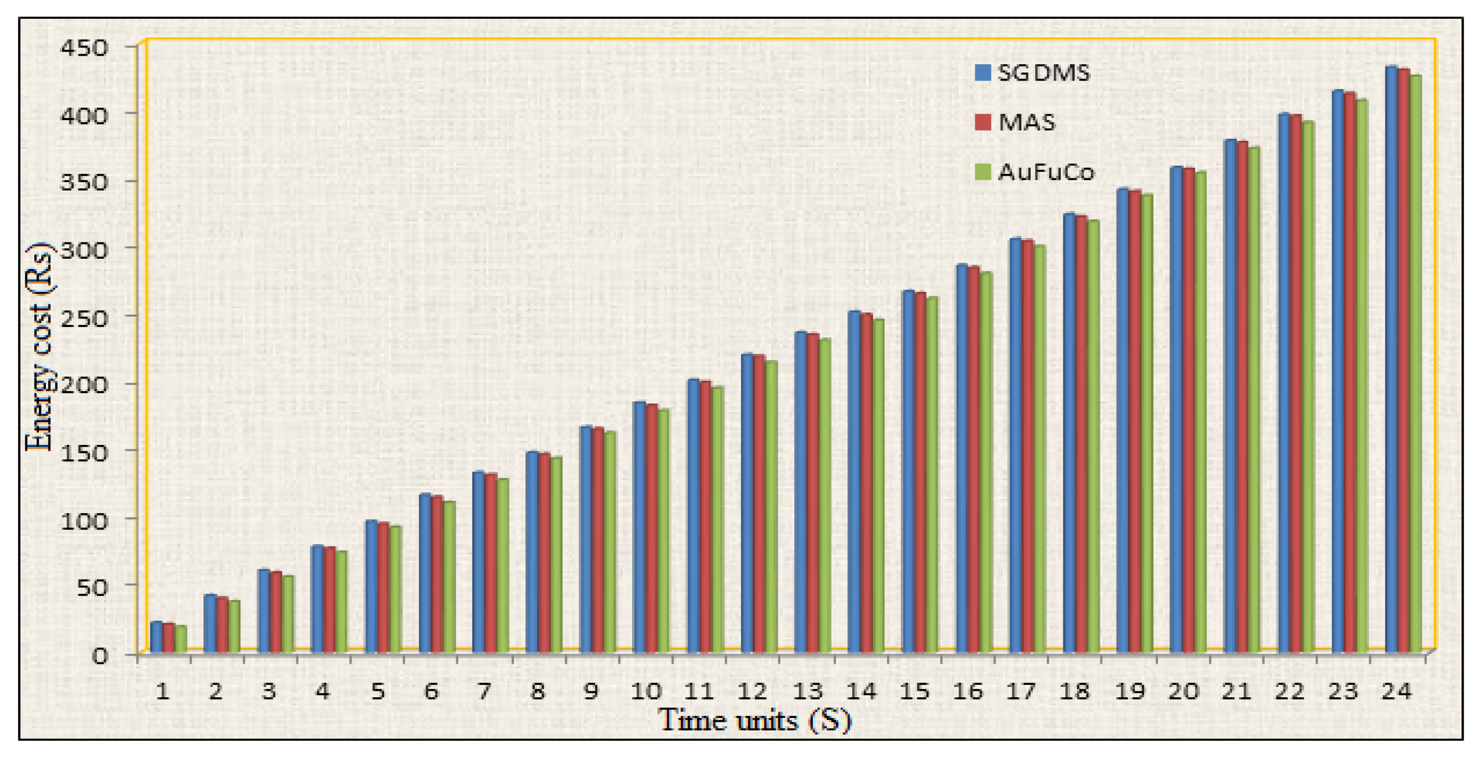
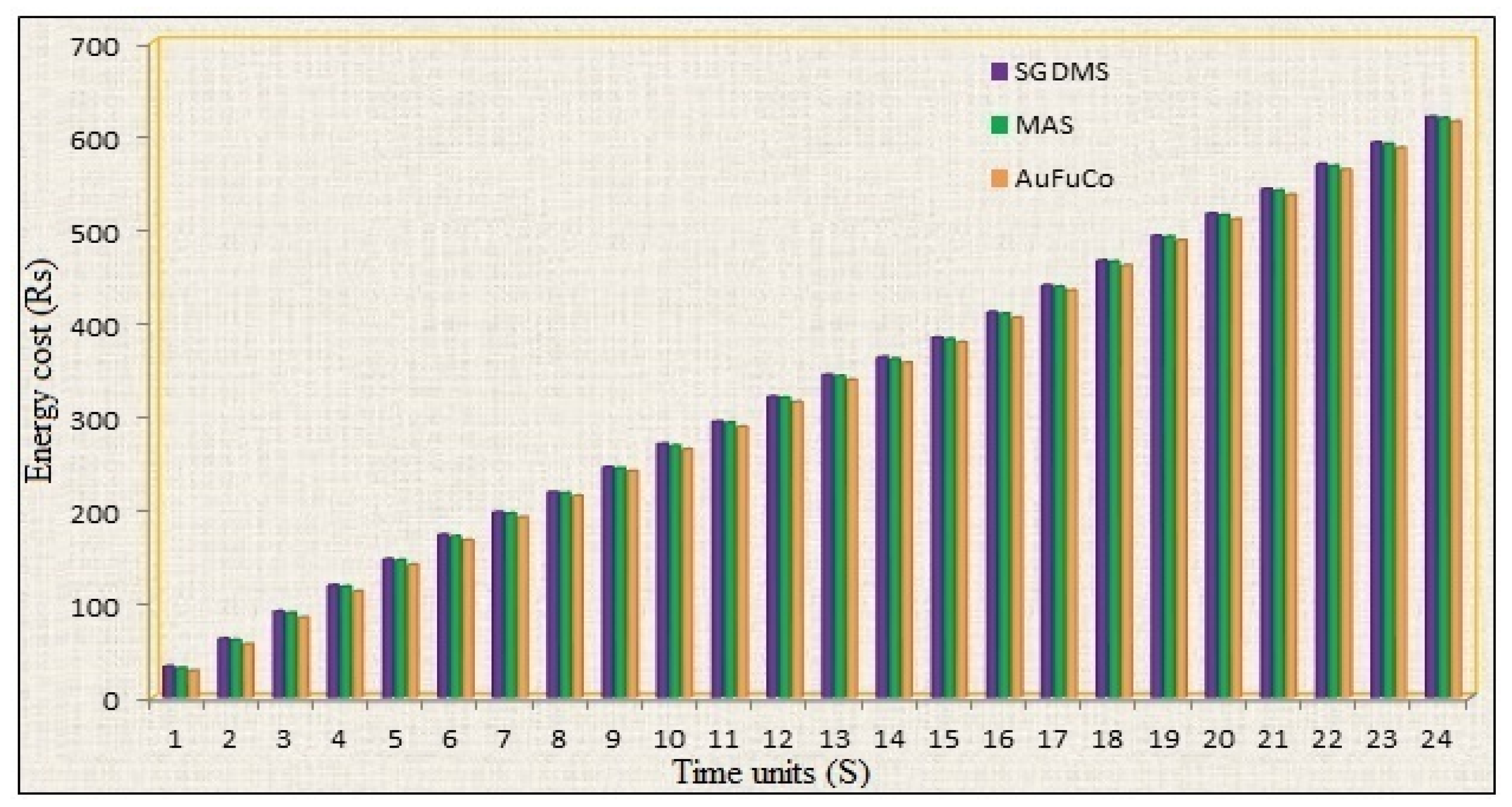
A multi-agent system (MAS)Presented a smart grid distribution management system (SGDMS) for contestable and non-contestable consumers. Multi-agent system (MAS) technology reduced the electricity price of consumers but foresting prices are not presented [24].
Integrated energy management systemReported an integrated energy management system (EMS) with PV, an electric vehicle, a battery, and thermal power storage devices with complex forecasting [25].
Artificial bee colony (ABC)Implemented an artificial bee colony (ABC) as an optimizer to improve the HEMS but cost optimization concepts are not incorporated [26].
Intelligent energy management systemA suggested intelligent energy management system that finds the optimal energy efficiency to maximize energy usage. However, energy forecasting and cost optimizations are not presented [27].
Energy controller systemAn implemented energy controller system to control household appliances such as air conditioners and lighting. The concepts of cost optimization with hybrid renewable sources are not incorporated [28].
Levelized cost functionSuggested Levelized cost of systems for electricity generation and reported that the cost can be reduced considerably with increased renewable energy penetration at no extra cost. However, individual energy and forecasting prices are not discussed greatly [29].
Table 2. List of main inputs for the simulation process.
PV InputsWind Power Inputs
Reference Temperature (Tref in °C)25.00Cut in speed (m/s)2.00
Operating Temperature range (Top in °C) 25.00–50.00Cut out speed (m/s)24.00
Solar Radiation variations (puW/m2)0.25–1.09Wind speed variations (m/s)0.00–24.00
PV Power variation (kWP)0.00–2.00Wind Power variation (kW)0.00–2.00
Table 3. Domestic consumer load classification.
Base LoadPriority Load
Appliance NameNumbers & individual Ratings (kW)Power Ratings (kW)Appliance NameNumbers & Individual Ratings (kW)Power Ratings (kW)
Refrigerator1 (0.50)0.50Air conditioning1 (1.50)1.50
Lights5 (0.04)0.20
Fan3 (0.08)0.24Heating load1 (0.50)0.50
Television1 (0.15)0.15
Computers1 (0.15)0.15
Total power (kW)1.24Total power (kW)2.00
Schedulable LoadShort Term or Burst Load
Appliance NameNumbers & Individual Ratings (kW)Power Ratings (kW)Appliance NameNumbers &Individual Ratings (kW)Power Ratings (kW)
Washing machine1 (0.50)0.50Mixer1 (0.50)0.50
Wet grinder1 (0.40)0.40Pump motor 1 (0.50)0.50
Iron box 1 (0.50)0.50Induction stove1 (1.00)1.00
Total power (kW)1.40Total power (kW)2.00
Table 4. Summary of results for the different source combinations.
Energy CombinationsPV and GridWind and GridPV, Wind, and GridGrid Supply
Energy
(kWh)
Cost
(USD)
Energy
(kWh)
Cost
(USD)
Energy
(kWh)
Cost
(USD)
Energy
(kWh)
Cost
(USD)
PV (EPV,t)13.23−0.550013.23−0.5500
Wind (Ewind,t)0014.10−0.5114.10−0.5100
Grid (Egrid,t)76.804.7085.905.2562.673.8396.045.87
Total (EtR)90.034.1599.224.7490.002.7796.045.87
Table 5. Domestic consumer energy tariff rates at the proposed location.
S. No.Energy BlockEnergy Cost /Unit
10–100 units (bimonthly) 0.034 USD/unit and no Fixed charges [No Energy bill scheme]
2101–200 units (bimonthly)0.048 USD/unit and fixed charges 0.410 USD/Service
3201–500 units (bimonthly) 0.063 USD/unit and fixed charges 0.540 USD/Service
4Above 501 units (bimonthly) till 1000 units 0.090 USD/unit and fixed charges 0.680 USD/Service
Table 6. Energy generation and tariff-based energy rates for domestic consumers.
Energy
Block
(kWh)
Wind Energy
(kWh)
PV Energy
(kWh)
Grid Energy
(kWh)
Total Energy
(kWh)
OptimumAverageOptimumAverageOptimumAverageOptimumAverage
0–10015.3617.3512.9013.2071.4672.7099.72103.25
101–20031.1134.7026.3826.70143.20138.60200.69200.60
201–30043.8052.0539.5840.30216.90207.70300.28300.80
301–50076.4086.6066.2069.20357.40344.20500.00513.20
501–1000161.80175.10142.10130.20709.40703.901013.301000.90
Table 7. Summary of results for the energy efficiency improvements.
Source CombinationsControllerWind Power Cost (USD)PV Power Cost (USD)Grid Power Cost (USD)Total Cost (USD)
Wind 45% and PV 23% efficiencySGDMS0.280.505.045.82
MAS0.270.495.025.78
AuFuCO0.270.495.005.76
Wind 35% and PV 18% efficiencySGDMS0.220.525.095.83
MAS0.220.525.085.81
AuFuCO0.210.515.075.78
Table 8. Hybrid PV-wind energy resources with grid supply: energy, power, and energy cost details for present and future scenarios.
Time Units
(S)
Forecasted Energy
(Units)
Generated
Energy
(Units)
Consumed
Energy
(Units)
Grid
Power
(kW)
PV
Power
(kW)
Wind
Power
(kW)
Energy Cost at Present (USD)Energy Cost by 2030 (USD)
Wind (USD)PV (USD)Total (USD)PV (USD)Wind (USD)Total (USD)
13.50003.70001.80003.200000.70000.01260.00140.26600.03280.00411.1767
28.80007.60003.70004.000000.30000.02240.00280.52780.05740.00412.3452
312.700011.90005.50004.0000000.02660.00420.78400.06560.00823.5014
415.600015.90008.30003.200000.60000.02660.00561.03740.06560.00824.6494
520.900019.700011.20004.000002.40000.03360.0071.29780.08610.01235.8138
626.900026.100015.70001.80001.80000.06720.01121.55260.17220.02056.8880
731.000029.700020.20000.60001.90000.06720.03221.78640.17220.05747.8925
835.100032.200024.70002.10001.9000.30000.06720.06022.01040.17220.11078.8314
940.300036.600029.20000.50001.90000.07280.09382.27220.18450.17229.9179
1044.400039.100033.70001.50001.90000.07280.13022.50320.18450.237810.8690
1147.300042.600038.20002.20001.8000.70000.07280.16242.73700.18450.295211.8490
1250.100047.300042.70001.00002.00000.08260.19183.00020.20910.352612.9390
1352.900050.300047.20004.00002.0002.50000.08260.22543.23120.21320.410013.9010
1456.700056.900051.70001.00002.0002.00000.11760.26183.43560.29930.479714.6540
1559.600059.800056.20001.70001.9000.60000.14560.29543.66240.36900.537115.5420
1662.500064.100060.70002.00001.9000.60000.15260.32063.92000.38950.586316.6250
1767.800068.500065.20003.00001.9000.90000.16100.33884.19580.41000.619117.8150
1873.200072.400069.70002.50001.8001.00000.17360.36124.45620.44280.660118.9020
1978.500075.900074.20002.600001.30000.18760.39624.72500.47560.721620.0110
2083.800079.800078.70004.000000.30000.20580.42984.95740.52070.783120.9370
2188.300084.100083.20004.000000.30000.21000.46065.21360.5330.840522.0080
2290.200088.400087.70004.0000000.21280.49705.47820.54120.906123.1050
2391.900092.400092.20004.0000000.21420.52365.70500.54530.955324.0690
2494.700096.400096.10003.900000.40000.21420.52505.95700.54530.955325.2190
Publisher’s Note: MDPI stays neutral with regard to jurisdictional claims in published maps and institutional affiliations.

