Abstract
Renewable sources of energy (RES), especially photovoltaic (PV) micro-sources, are very popular in many countries. This way of clean power production is applied on a wide scale in Poland as well. The Polish legal regulations and tariffs specify that every prosumer in a low-voltage network may feed this network with a power not higher than the maximum declared consumed power. In power networks with RES, the voltage level changes significantly along the power line and depends on the actually generated as well as consumed power by particular prosumers. There are cases that prosumers connected to this line cannot produce and inject the full permissible power from PV sources due to the level of a voltage higher than the technically acceptable value. In consequence, it leads to the lack of profitability of investments in installations with PV sources. In this paper, voltage variations in a real rural low-voltage network with PV micro-sources are described. The possible two general solutions of voltage levels improvement are discussed—increase in the cross-sectional area of the bare conductors in the existing overhead line as well as the replacement of the overhead line with a cable line. The recommended solution for the analyzed network, giving the best reduction of voltage variations and acceptable cost, is underlined. Such a recommendation can also be utilized in other rural networks.
1. Introduction
In recent years, a significant increase in the number of installed photovoltaic (PV) sources has been noticed. According to the report from 2019 [1], photovoltaic energy sources produce almost 1200 MW in Poland. PV sources are the most popular renewable energy sources (RES) among prosumers [2], especially in the so-called micro-installations (up to 50 kW). In general, the weather-related instability of PV energy production is a problem for the entire power system [3]. Moreover, as the power of installed micro-sources in the distribution network increases, problems begin to appear related to maintaining the required voltage. During the peak of the power generation by PV sources, the energy consumption by prosumers is most often low. These phenomena lead to a voltage level that exceeds the permissible value. According to the national legal regulation [4] and standard EN 50160 [5], the permissible range of the network voltage is (0.9–1.1) Vn, where Vn is the nominal voltage of the network. Furthermore, too high a voltage in the network may cause automatic disconnection of PV sources, which disables the production of clean power and is unfavorable from the economical point of view.
The discussed state of affairs was presented in publications [6,7]. The problems most often concern rural networks, which are characterized by long circuits [8,9]. For the network analyzed in the paper [10], it was shown that only with a 20% share of power generation by PV sources installed in the low-voltage (LV) network, no voltage problems were noted. Therefore, it seems to be reasonable to apply restrictions regarding the maximum installed power of renewable sources. In Poland, this limitation is defined by the maximum declared consumed power, which, according to [4,11], is active power drawn or injected into the network based on the concluded contract. In turn, the contracted power may not exceed the power for which the line supplying a consumer has been designed. It has been proved in the article [12] that limitations regarding the installed power of PV sources cannot be rigid because voltage problems for each network start at a different power value of these sources. The voltage problems depend on, among others, the length of the circuits, cross-sections of the power lines, load profiles and the location of the PV source. An interesting idea is to specify the active power limit that can be used for voltage control purposes, as shown in the paper [13].
In the power system, the topic related to voltage variations/deviations is important—it initiates the search and study of the possibility of reducing voltage variability [14]. In order to reduce too high voltage level in the distribution network resulting from the production of power by PV sources, the following solutions are considered/applied nowadays:
- The reconfiguration of the LV network or construction of new LV networks in such a way that the LV power lines supplying consumers are as short as possible. Such assumptions can be taken into account when a new power infrastructure is built, as presented in the paper [15]. For economic reasons, such a method is not feasible in the situation of the existing power infrastructure due to the necessity to add/relocate medium-voltage/low-voltage (MV/LV) power substations, demolition of existing lines and construction of new ones.
- The application of the on-load tap changer on a transformer in the MV/LV power substation. This solution is presented in papers [16,17]. Such control of voltage is justified when the entire LV network is saturated with PV sources. If at least one circuit from the power substation has no PV sources, it may turn out that the voltage at this point in the network will be inappropriate. The control is global in nature and does not reduce voltage problems occurring along the power line.
- Control the reactive power at the photovoltaic sources. Due to the possibility of receiving/supplying reactive power by the inverter, it is possible to control the voltage in the network—such a solution is presented in papers [18,19,20,21]. The disadvantage of this solution is that, due to the significantly higher value of resistance over reactance in the LV network, the control is carried out in a narrow range. Some solutions combine both local voltage control by inverters in the depth of the network and global control by an on-load tap changer [22,23]. However, such a method of control requires the possibility of making the device, which is an inverter belonging to the customer but available to the Distribution System Operator (DSO). Additionally, the solution requires sophisticated communication systems that allow sharing information between power network components about their state, taking into account various transmission disturbances. In such networks, a fully distributed cooperative control protocol, as presented in [24], which allows for appropriate cooperation of devices in the power network, can be utilized. Unfortunately, such a solution involves additional costs related to the use of special data transmission and processing technologies.
- The use of energy storage units and, thus, control over the flow of active and reactive power in the network. This solution has been heavily analyzed in recent years. There are many publications on this subject, including [25,26,27,28,29]. It should be noted here that the cost of this solution is high. Additionally, the estimated lifetime of energy storage units is not long, approx. 10 years. Therefore, the question arises whether it is not more economical to replace the power lines with larger cross-section lines, which can be utilized for at least 25 years.
- The identification of places/nodes in the network where it is possible to install PV sources or limit the produced power. These methods are not used in practice because they assume unequal treatment of consumers in terms of the possibility of generating power by renewable sources.
- The use of electric vehicles—especially since electric vehicle charging techniques are becoming more and more advanced and user-friendly [30]. However, it will take time to implement these solutions in many countries, and the power network problems related to PV sources are already present.
- Replacement of power lines with larger cross-section lines. This method does not involve placing additional devices in the network that require additional maintenance. Additionally, it does not require a complete reconstruction of the network in overhead lines, and it may be enough to replace the wires. It is clearly simpler than the reconfiguration mentioned in point 1. The authors’ investigation is focused on this method.
This article presents an analysis of the voltage conditions in a real rural low-voltage network located in northern Poland. The analysis of the current state of this network shows that in the case of no PV generation, the voltage in some nodes may be very close to the lower permissible limit (0.9 Vn). However, when PV generation is active, the voltage may exceed the upper permissible limit (1.1 Vn). The solutions that enable a decrease in voltage variations, especially that enable keeping them within the permissible normative range, are proposed. The most suitable solution related to the voltage improvement, which can be implemented by the operator of the analyzed network, is expressed.
The rest of this paper is organized as follows. In Section 2, the description of the analyzed real low-voltage network and its computer model are presented. Section 3 discusses the effect of the increase in the cross-sectional area of the bare conductors on the voltage variations, the possibility of voltage variations reduction by the replacement of the overhead line with a cable line as well as includes economic calculations. Conclusions flowing from the investigations, along with the recommendation for the operator of the analyzed network, are included in Section 4.
2. Materials and Methods
2.1. Description of the Analyzed Network
The analyzed low-voltage network is an overhead rural network in which the main supply line is 4 × AL 35 mm2 (four-wire, aluminum bare conductors of nominal cross-sectional area 35 mm2). The farthest prosumer is 1.15 km away from a 15/0.4 kV power transformer substation. The loads are mainly single-family or summer-holiday houses (profile 3 and 4, respectively—Figure 1). Other loads are a shop and small farms, which correspond to load profiles 2 and 1, respectively (Figure 1). The maximum declared consumed power of individual loads is presented in Table 1. To perform the computer analysis, the profiles of the loads from Figure 1 were assumed.
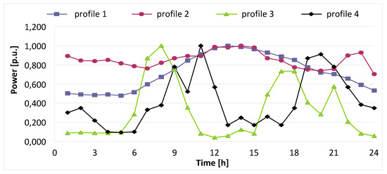
Figure 1.
Assumed profiles of the loads: profile 1: shop; profile 2: agricultural; profile 3: detached house; profile 4: detached (summer) house.

Table 1.
The maximum declared consumed power by loads in the analyzed network.
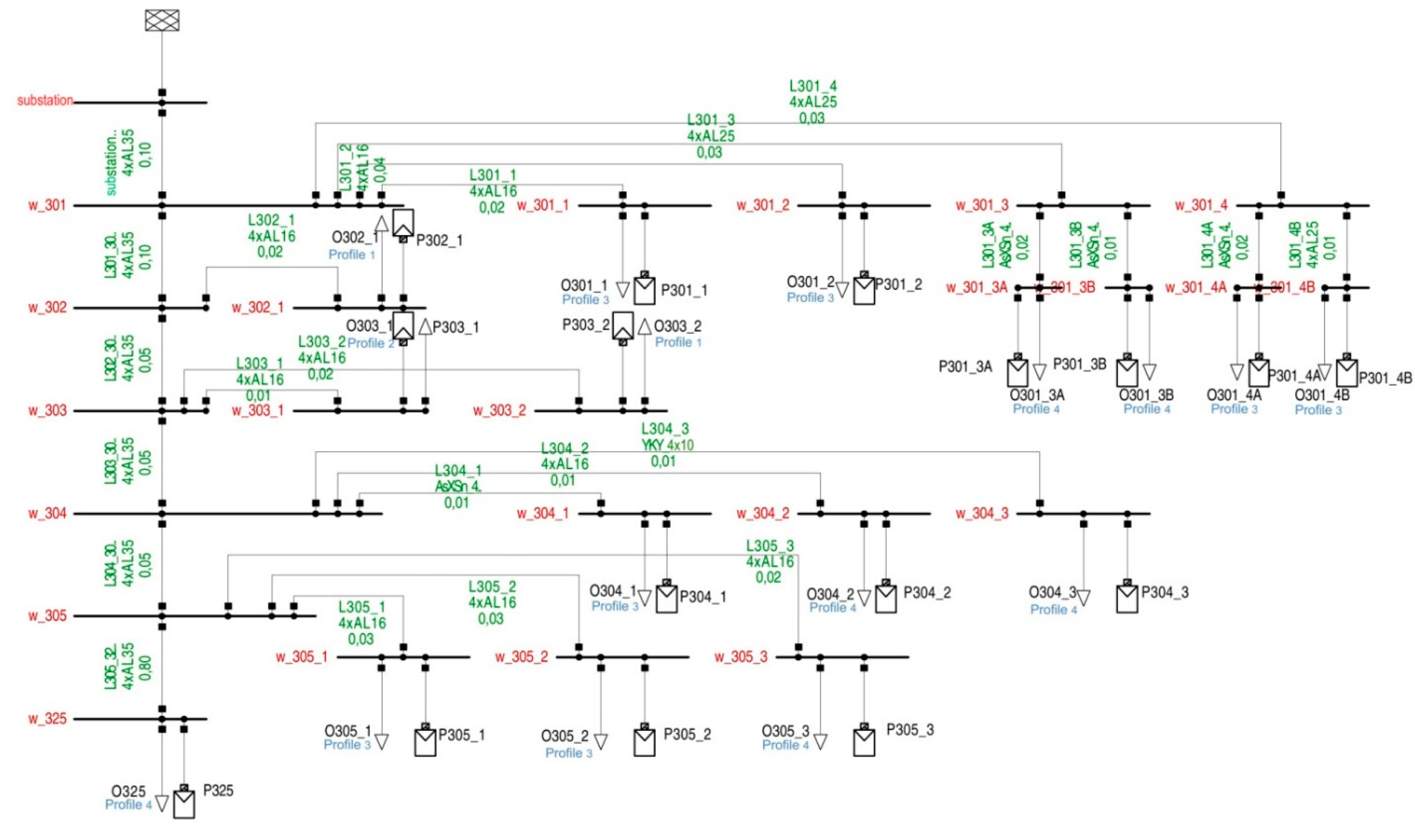
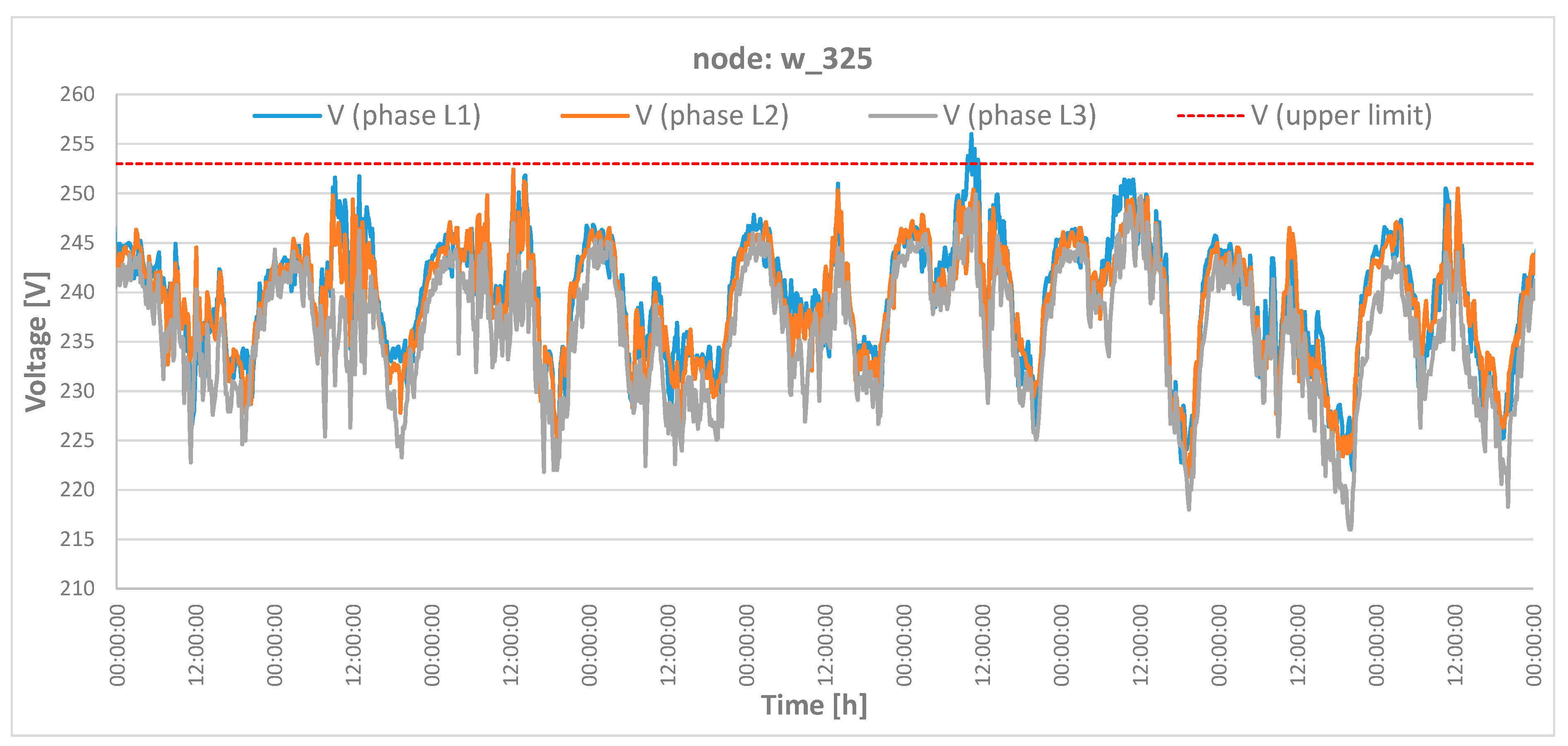
The maximum permissible generated power is equal to the maximum consumed power [11]. The modelled structure of the analyzed low-voltage network is depicted in Figure 2. For the node relatively far from the transformer substation (node w_325), daily voltage variations have been measured (Figure 3). One can see that these variations (recorded for 9 days) are within the wide range and even exceed the upper permissible limit (dashed trace). It is an example to show that voltage variations/deviations in this network may really exceed the upper limit, which is unacceptable. Therefore, this real low-voltage network was modelled to perform extended voltage analysis.
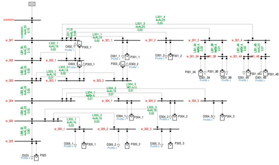
Figure 2.
A diagram of the analyzed low-voltage network. Example symbols: Numbers of nodes: w_301, w_301_4 and w_325; section of the main distribution line between nodes w_301 and w_302: L301 302; power line supplying node w_301_4: L301_4; 4 × AL16: overhead line composed of 4 bare aluminum conductors of cross-sectional area 16 mm2; AsXSn4: overhead line composed of 4 insulated aluminum conductors; YKY 4 × 10: cable line composed of 4 copper conductors of cross-sectional area 10 mm2; O301_1, Profile 3: modelled load in node w_303_1, the prosumer has profile 3 (see Figure 1); P301_1: modelled PV generation in node w_301_1; 0.10 and 0.06—the length of the power line, 0.10 km and 0.06 km, respectively.
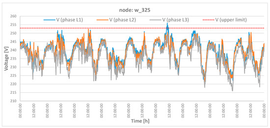
Figure 3.
Measured voltage-to-neutral (August 2020, 10-min average) at node w_325 in the analyzed network of the nominal voltage 230 V (daily variations of voltage recorded for 9 days).
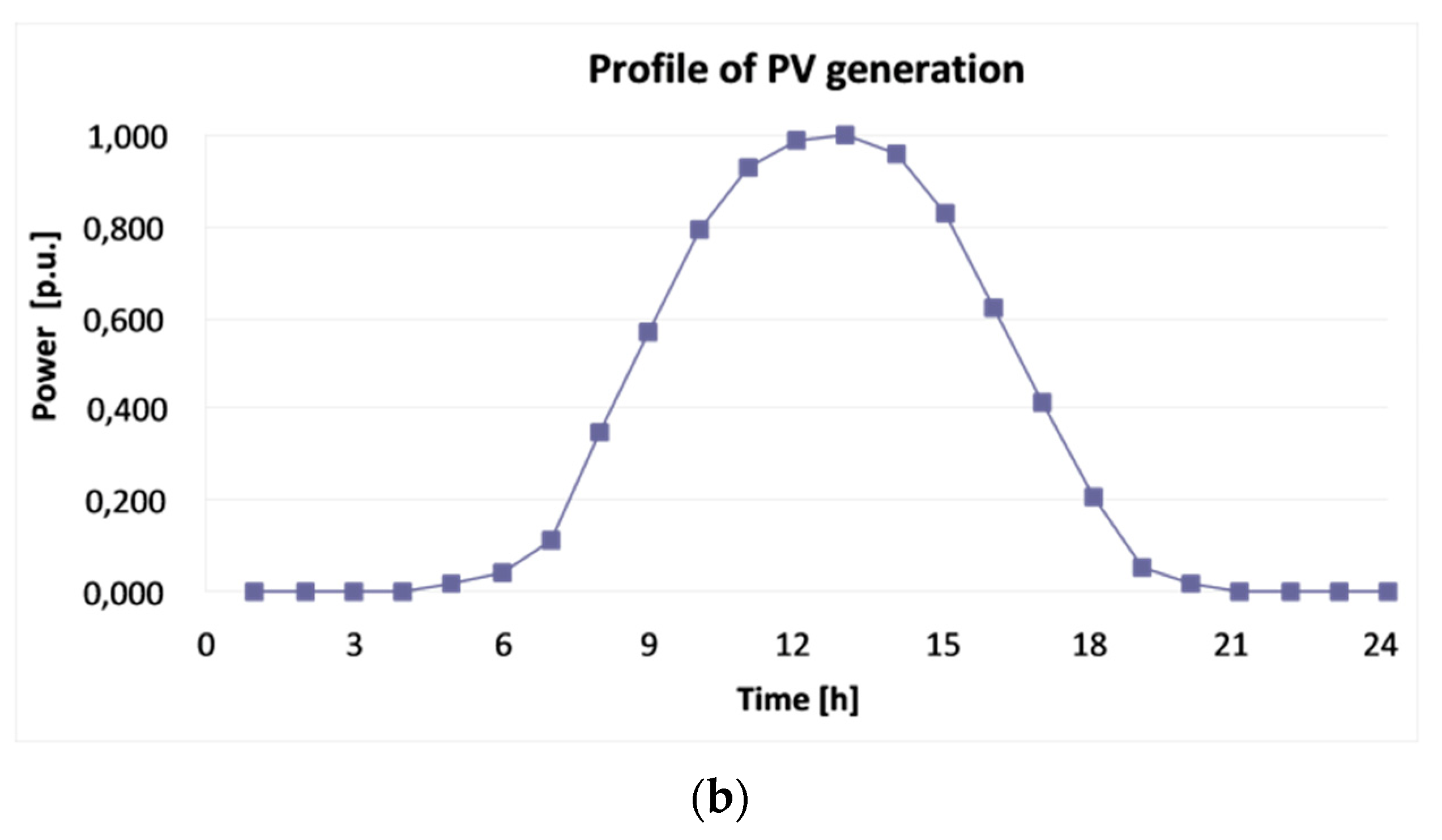
The main line, which parameters are changed in subsequent computer simulations, runs from the substation node to node w_325 (Figure 2). Connections to prosumers or another intermediate node depart directly from the selected nodes. The network is a radial type. The analyzed low-voltage network has been modelled with the use of DIgSILENT Power Factory software. Voltage conditions (daily variation) in selected nodes (w_301—nearest to the transformer; w_303—in the middle of the main line; w_325—at the end of the main line) for the current network status are presented in Figure 4a, whereas Figure 4b presents assumed daily profile of the PV generation.
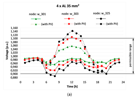
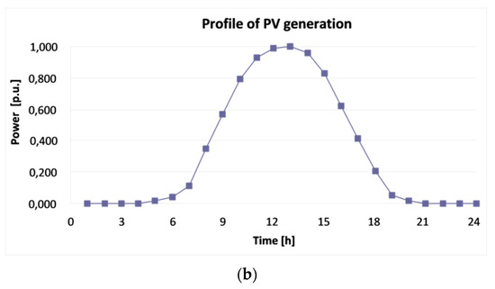
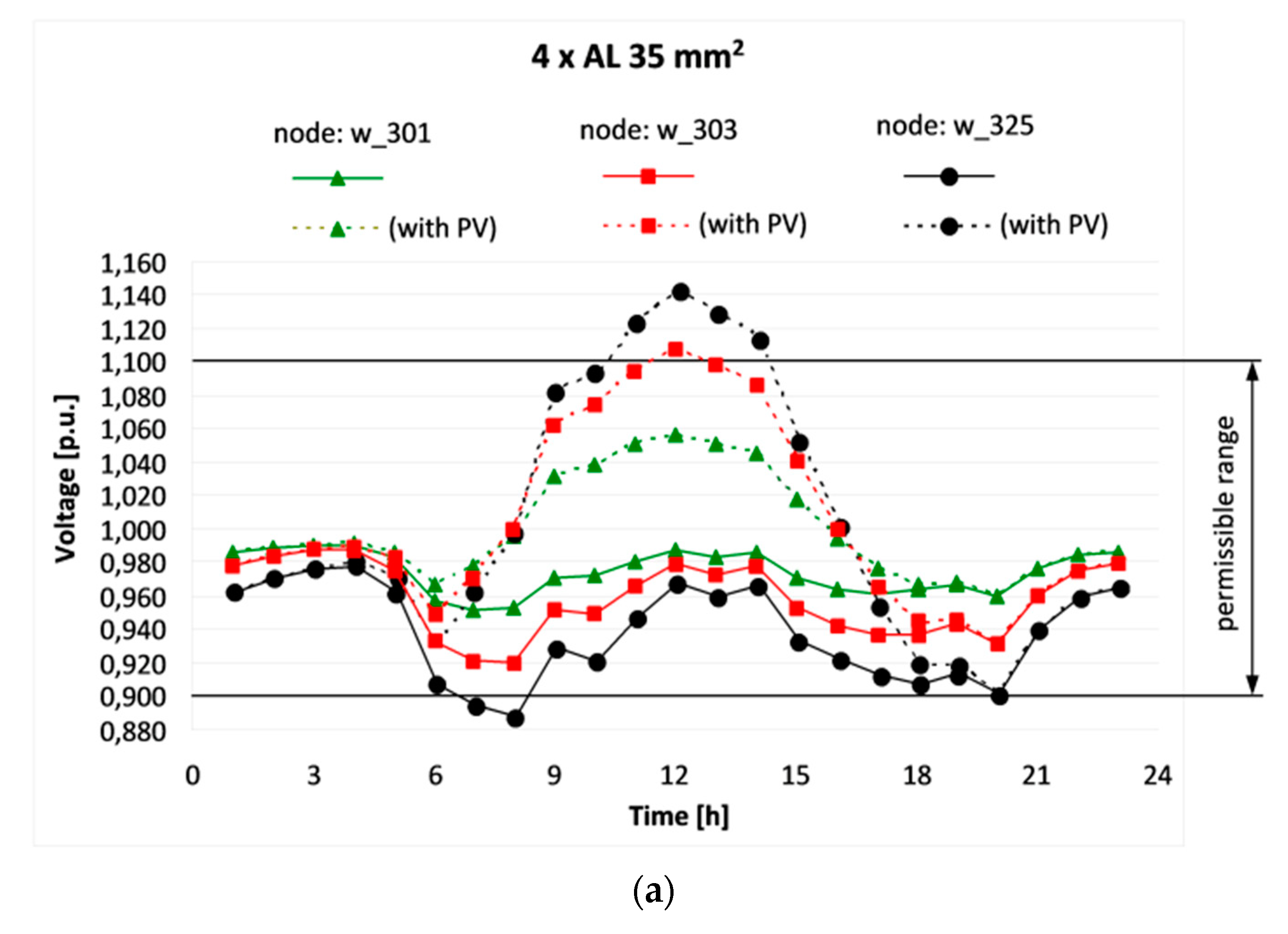
Figure 4.
Daily voltage variations in selected nodes w_301, w_303 and w_325 (a) and the daily profile of PV generation (b).
The most favorable voltage conditions are observed in node w_301 (Figure 4a). For the whole day (24 h), the voltage is within the permissible range—the lowest voltage is around 0.95 Vn (the case without PV generation, ca. 7:00 a.m.), and the highest voltage is almost 1.06 Vn (the case with PV generation, ca. 12:00 p.m.). A much wider range of voltage is noted in the case of node w_303. Moreover, during the maximum PV generation, the voltage value exceeds the upper permissible level of 1.1 Vn. The worst voltage conditions are observed in node w_325. This node (w_325) is far from the transformer (1.15 km) and, due to the voltage drop, the voltage at the period 7:00 a.m.—8:00 a.m. is below permissible 0.9 Vn. What is worse, during the period with the maximum PV generation (11:00 a.m.—2:00 p.m.), the voltage value significantly exceeds permissible 1.1 Vn. It may lead to the damage of the prosumer’s current-using equipment. Additionally, PV generators can be disconnected automatically. The voltage conditions in the analyzed network are not acceptable, so local DSO is searching for the solution, which in a relatively simple way could improve levels of voltage.
2.2. General Assumptions
To improve voltage conditions in the analyzed low-voltage network, the following main solutions are considered:
- Replacement of the actually utilized bare conductors of the overhead main line 4 × AL 35 mm2 with bare conductors consecutively: 4 × AL 50 mm2, 4 × AL 70 mm2;
- Replacement of the overhead main line 4 × AL 35 mm2 with a cable line YAKY 4 × 35 mm2.
The aforementioned first solution makes that the reactance of the line practically does not change, but the resistance decreases significantly. In the second solution, the line resistance is almost constant, but the reactance decreases around 4 times. As an extension, the effect of cables YAKY 4 × 50 mm2 and YAKY 4 × 70 mm2 is also analyzed. Table 2 presents the nominal parameters of the overhead lines and the cable lines.
Table 2.
Nominal parameters of the considered bare conductors and cable lines.
Voltage conditions along a line mainly depend on the voltage drop in it. Figure 5 presents the general relation between voltages in two nodes. Voltage VfB at node B depends on the geometric difference of the voltage phasor VfA at node A and the voltage drop ΔVAB across the A-B section. Due to the fact that for MV and LV networks, the angle β reaches small values (VfA ∙ cos(β) ≈ VfA), the following formula can be used to calculate the voltage at node B:
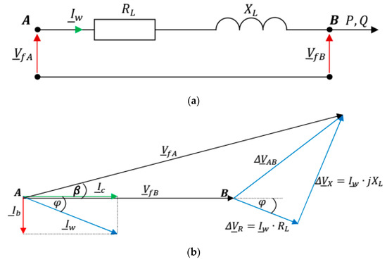
Figure 5.
Simplified equivalent circuit (for a single-phase) between nodes A and B (a), and its phasor diagram (b); VfA—line-to-neutral voltage in node A; VfB—line-to-neutral voltage in node B; RL—resistance of the section A-B; XL—reactance of the section A-B; ΔVAB—voltage drop between nodes A and B; ΔVR—voltage drop between nodes A and B across the resistance of the line; ΔVX—voltage drop between nodes A and B across the reactance of the line; Iw—load current in the line; Ic—the active component of the load current; Ib—reactive component of the load current; P—active power flow; Q—reactive power flow.
VfA—line-to-neutral voltage in node A;
VfB—line-to-neutral voltage in node B;
RL—resistance of the section A-B;
XL—reactance of the section A-B;
P—active power flow (consumed at node B);
Q—reactive power flow (consumed at node B).
Based on the aforementioned description (Figure 5 and Equation (1)), the computer simulation assumes that PV sources generate only active power (it refers to practice), so the voltage drop in the line is affected by its resistance. During consumption of energy, the assumed load reactance-to-resistance ratio is 0.2.
3. Results
3.1. Increase of the Cross-Sectional Area of the Bare Conductors in the Main Line
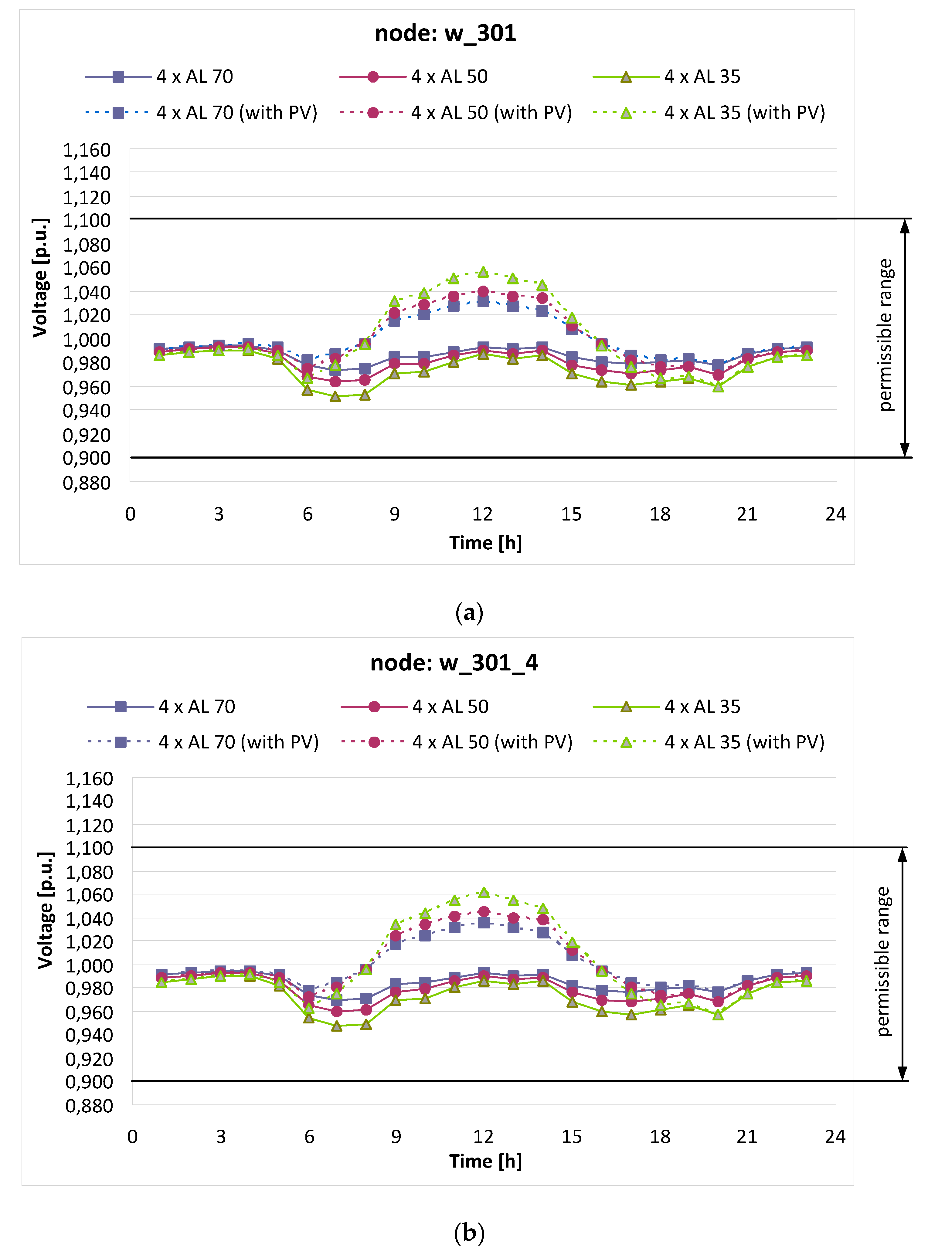
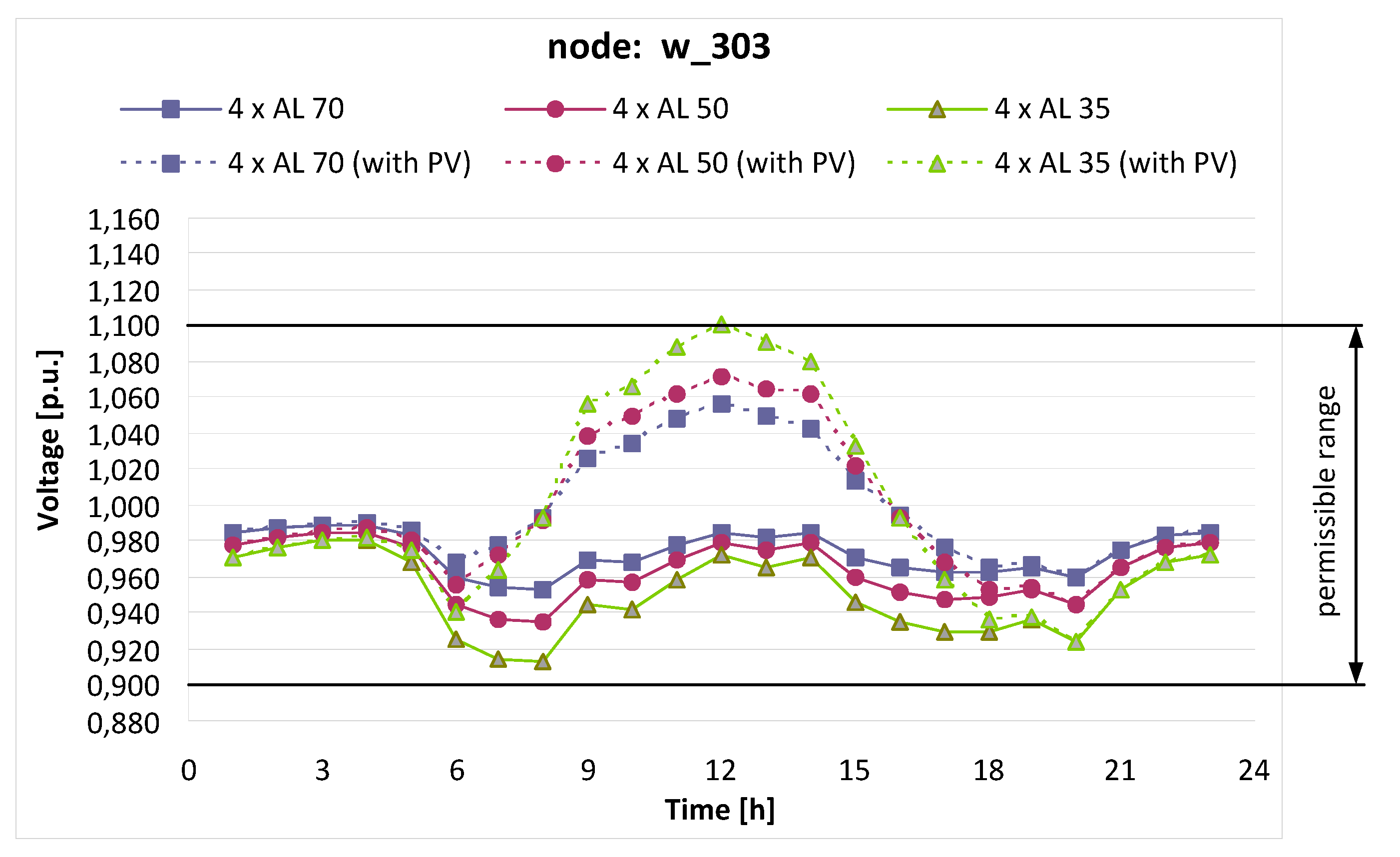
Figure 6, Figure 7, Figure 8 and Figure 9 present daily variation of the voltage in selected nodes for various cross-sectional areas of bare conductors without PV generation as well as with PV generation. For the nodes that are located relatively close to the transformer substation (Figure 6—nodes w_301 and w_301_4), voltage variations are quite narrow for all the cases (35 mm2, 50 mm2 and 70 mm2). Node w_303 (Figure 7) has worse voltage conditions but acceptable from the normative point of view (voltage is within the range 0.9–1.1 Vn).
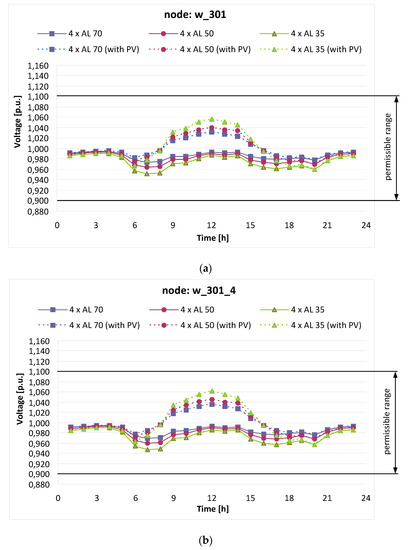
Figure 6.
Daily voltage variations in nodes: (a) w_301 (node nearest the transformer substation); (b) w_301_4; for three variants of the overhead bare conductors of the main line: 4 × AL 35 mm2, 4 × AL 50 mm2 and 4 × AL 70 mm2.
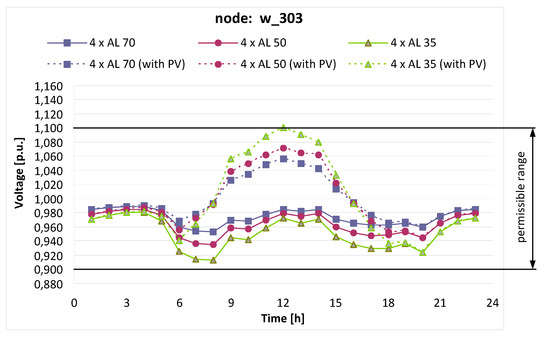
Figure 7.
Daily voltage variations in node w_303 for three variants of the overhead bare conductors of the main line: 4 × AL 35 mm2, 4 × AL 50 mm2 and 4 × AL 70 mm2.
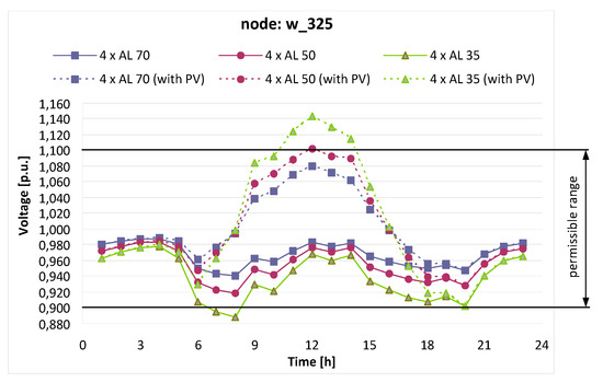
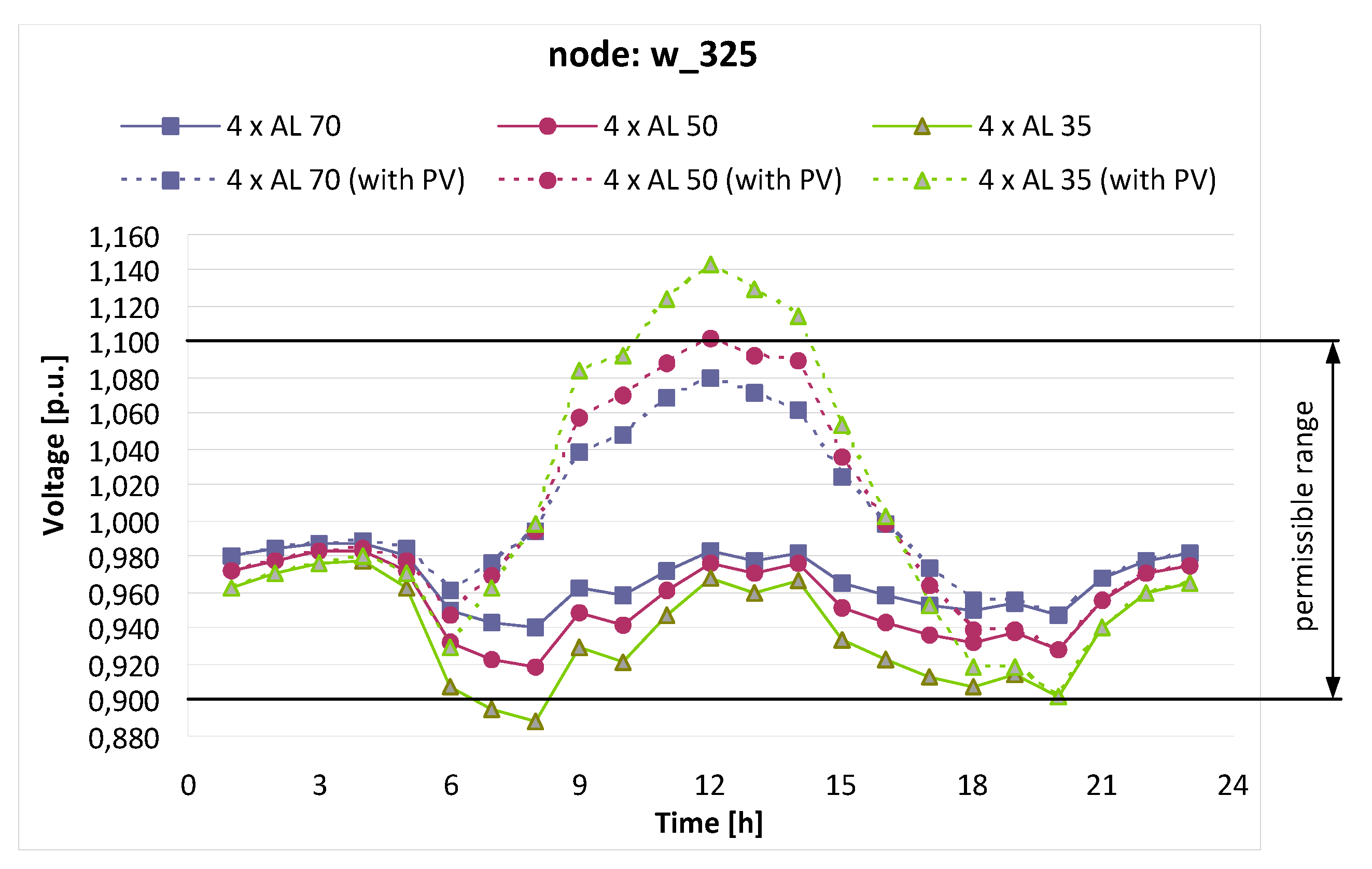
Figure 8.
Daily voltage variations in node w_325 (end of the main line) for three variants of the overhead bare conductors of the main line: 4 × AL 35 mm2, 4 × AL 50 mm2 and 4 × AL 70 mm2.
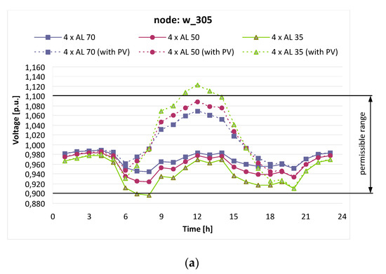
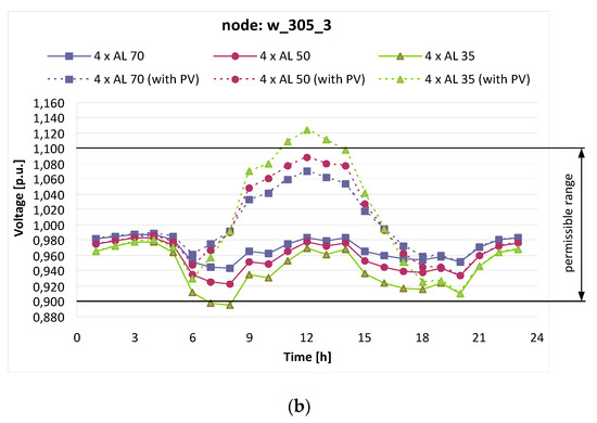
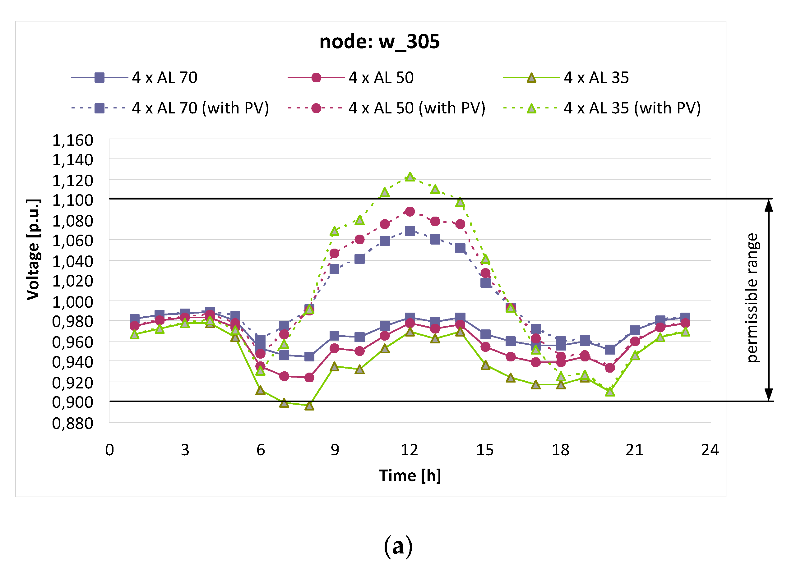
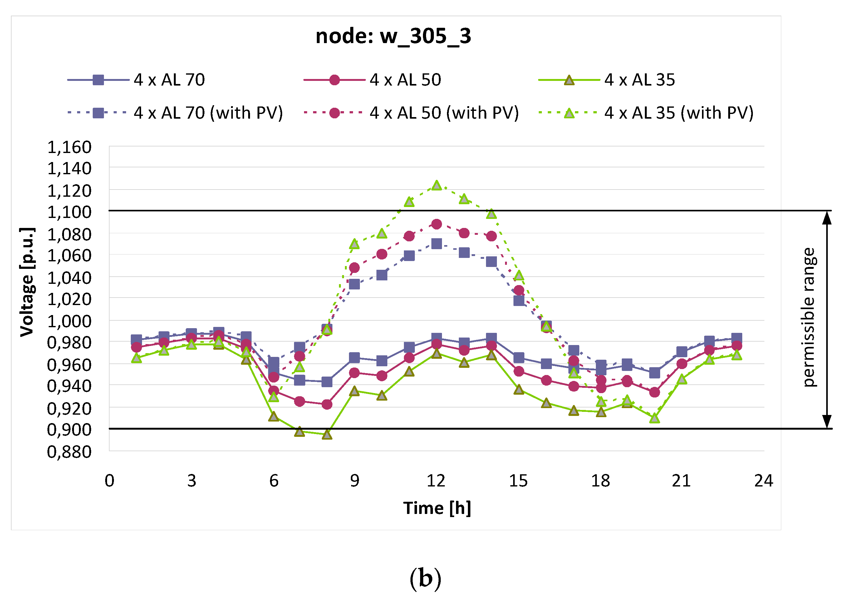
Figure 9.
Daily voltage variations in nodes: (a) w_305; (b) w_305_3; for three variants of the overhead bare conductors of the main line: 4 × AL 35 mm2, 4 × AL 50 mm2 and 4 × AL 70 mm2.
In the case of the nodes w_325 (Figure 8), w_305 and w_305_3 (Figure 9), the voltage exceeds the permissible range (in selected periods of the day) when the cross-sectional area of the conductors is equal to 35 mm2. For other cross-sections (50 mm2, 70 mm2), the voltage varies in the permissible range.
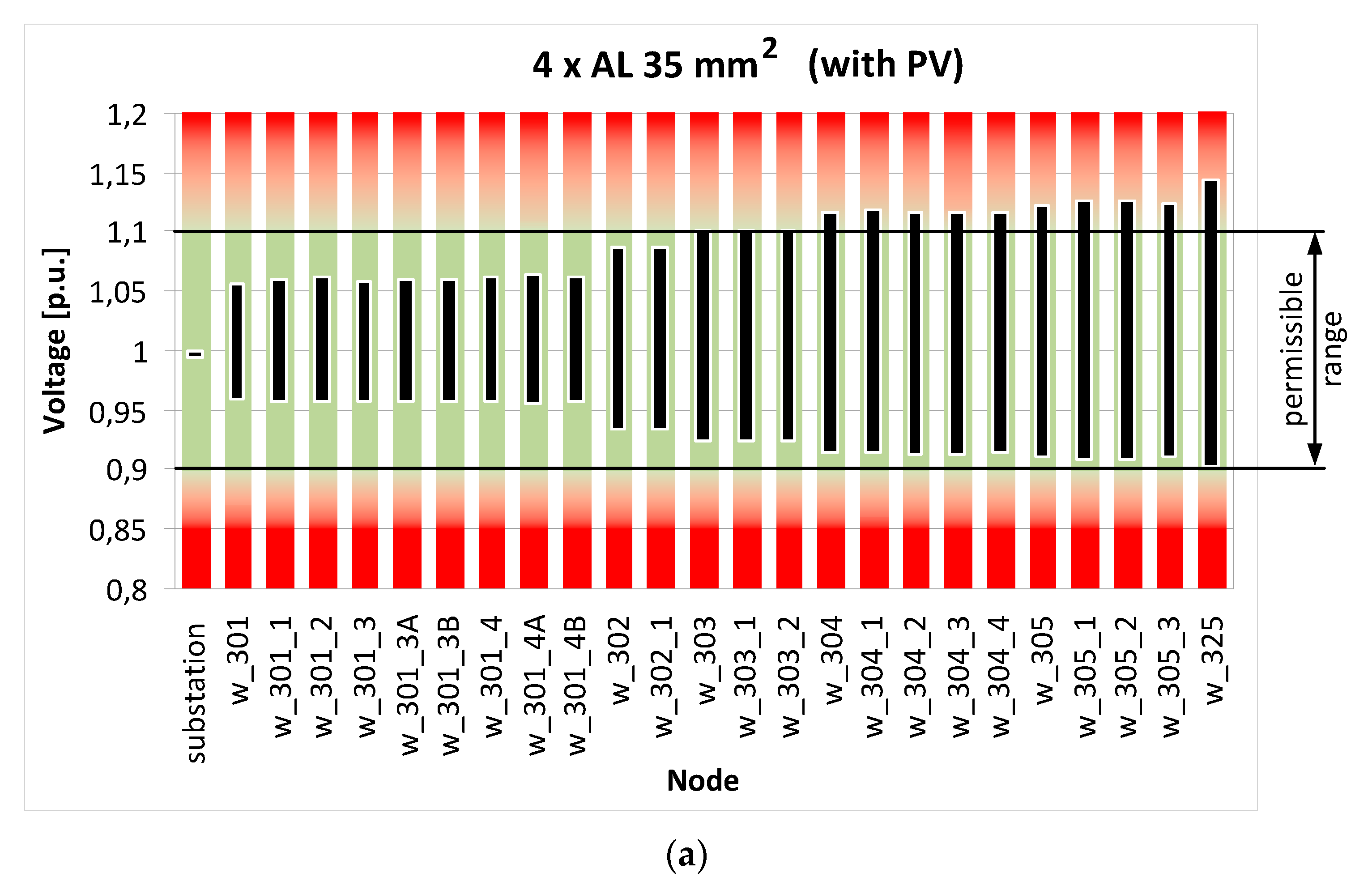
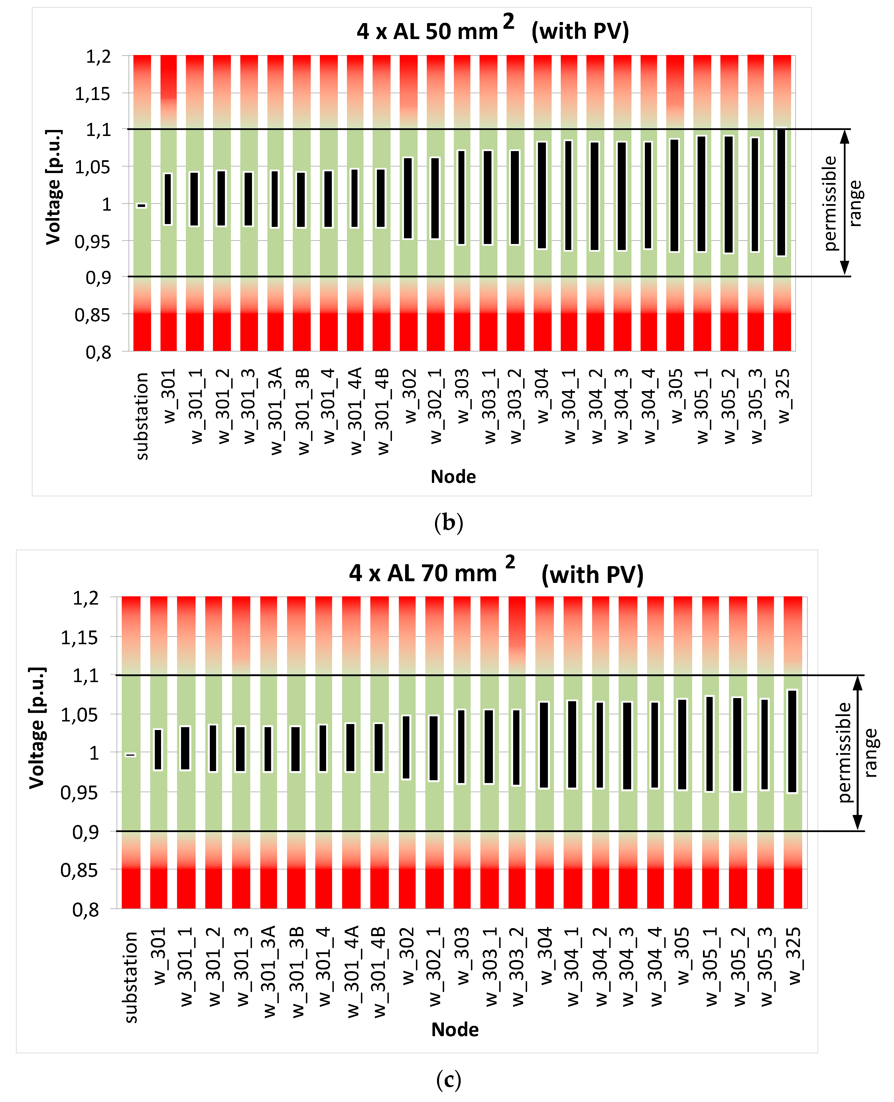
Aggregated results of the voltage variations for the cross-sections 35 mm2, 50 mm2 and 70 mm2 are presented in Figure 10. The highest voltage variations are at node w_325—the farthest analyzed node from the power transformer substation.
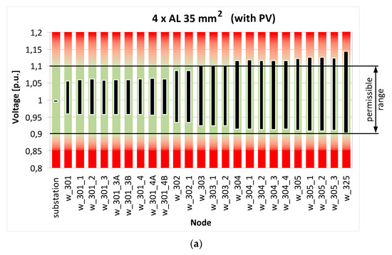
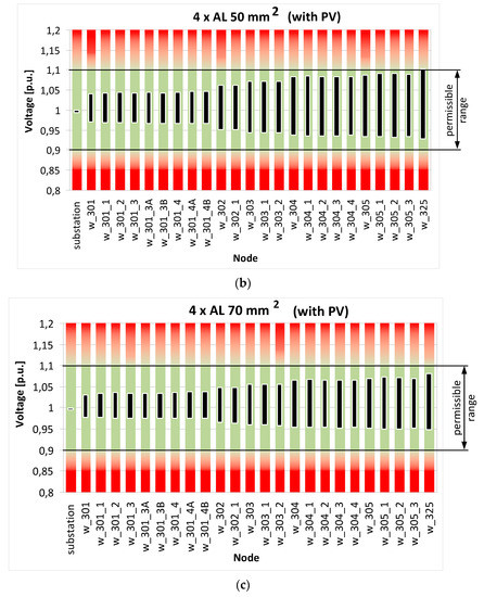
Figure 10.
Aggregated results of the daily voltage variations (vertical black bars) for all nodes, during PV generation, for the following cross-sectional areas of the bare conductors of the main line: (a) 4 × AL 35 mm2; (b) 4 × AL 50 mm2; (c) 4 × AL 70 mm2.
The voltage variations in the main line are the critical point of concern because, for radial power networks, they are of the greatest importance from the voltage stability point of view. If there are no significant voltage variations in the main line, the branches can be analyzed then. Figure 10a shows that the highest voltage variations (especially changes from node to node) are in the main line—compare relative changes in the main line (e.g., node w_301 vs. node w_302) and relative changes in the branch line (e.g., node w_301 vs. nodes w_301_1/w_301_2/w_301_3). Therefore, it is reasonable to reduce the voltage variations/deviations by the main line modernization.
It is clearly seen that replacing currently installed conductors 4 × AL 35 mm2 with conductors 4 × AL 70 mm2 gives a positive result, and voltage variations are limited to the acceptable range (with some excess) in every node. Thus, taking into account the obtained results, one can conclude that the decrease in the line resistance results in a significant decrease in the voltage variation/deviations in the considered network.
3.2. Replacement of the Overhead Line with a Cable Line
As an alternative to the low-voltage overhead line, a cable line can be installed. Such a solution is favorable from the point of view of the reliability of supply but requires that the power line is completely rebuilt. In the computer simulations, a cable line, as an alternative to the overhead line with the same cross-section, is considered. The investigation aims to verify the effect of the power line reactance reduction on voltage variations.
The results of the simulations for two selected characteristic nodes: w_301 and w_325, are presented in Figure 11, Figure 12 and Figure 13. In each case, both compared power lines (overhead AL vs. cable YAKY) have the same nominal cross-sectional areas of the conductors (almost the same resistance), but the cable line reactance is around 4 times lower than the overhead line (see Table 2). On the basis of these simulations, one can conclude that a significant decrease in the line reactance (the use of the cable line instead of the overhead line) does not give the expected result.
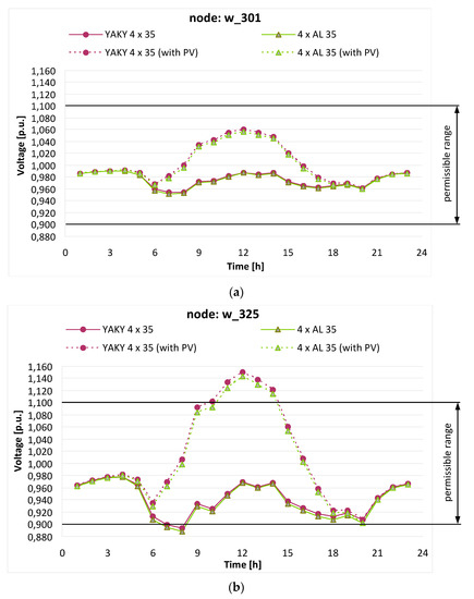
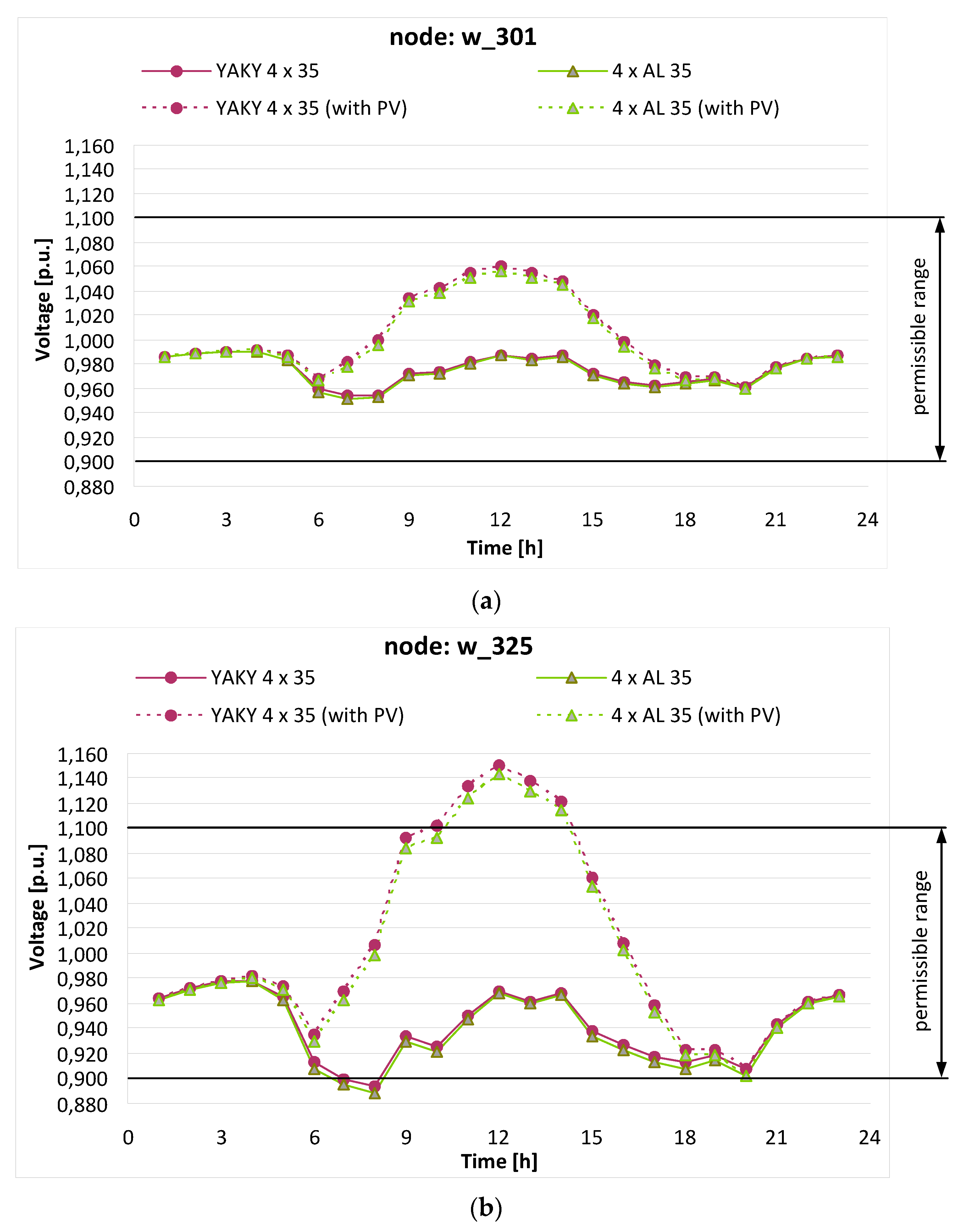
Figure 11.
Daily voltage variations in nodes: (a) w_301; (b) w_325; for two variants of the main line: overhead line 4 × AL 35 mm2 vs. cable line YAKY 4 × 35 mm2.
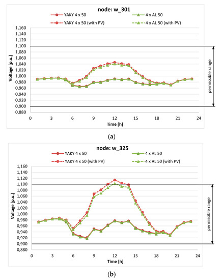
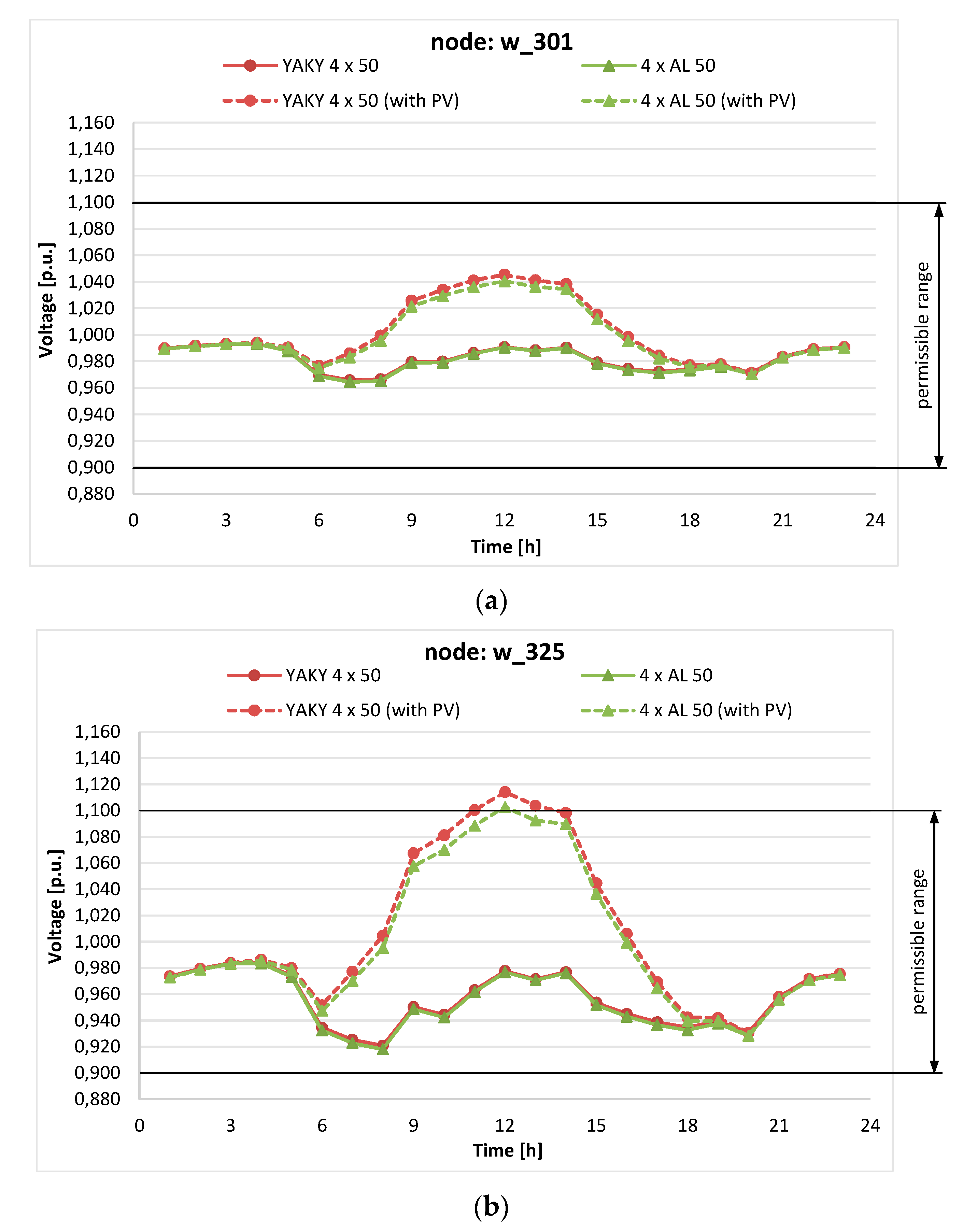
Figure 12.
Daily voltage variations in nodes: (a) w_301; (b) w_325; for two variants of the main line: overhead line 4 × AL 50 mm2 vs. cable line YAKY 4 × 50 mm2.
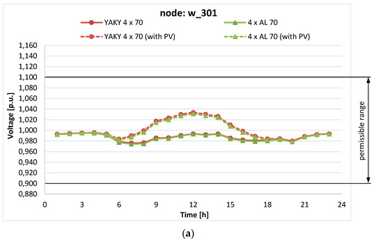
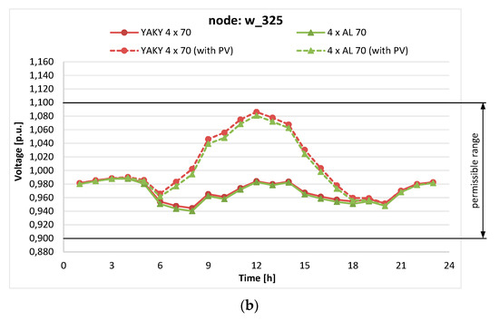
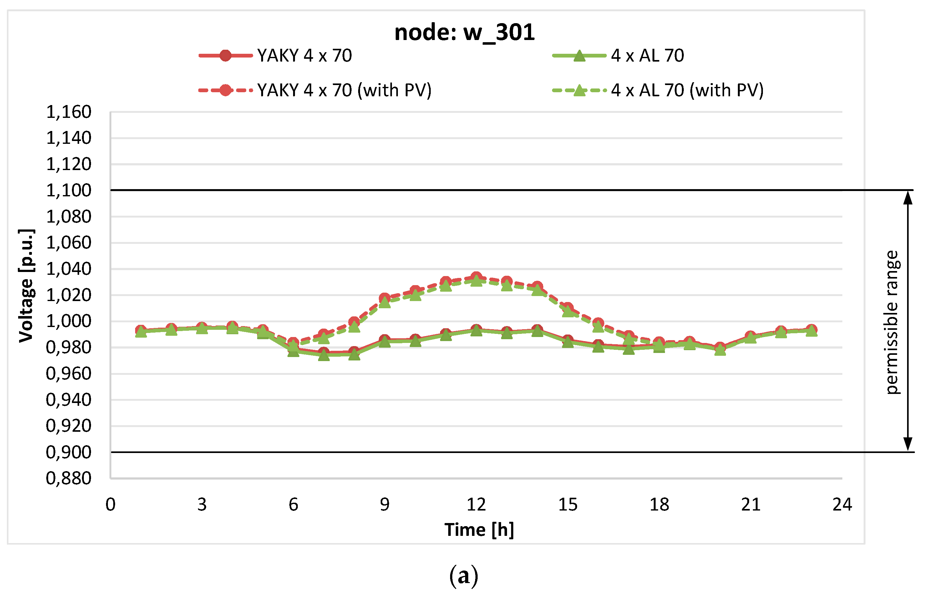
Figure 13.
Daily voltage variations in nodes: (a) w_301; (b) w_325; for two variants of the main line: overhead line 4 × AL 70 mm2 vs. cable line YAKY 4 × 70 mm2.
Generally, the voltage is slightly higher than for the overhead line, but in the case of high PV generation, this further aggravates the voltage conditions in the network. In the case of node w_325, during the highest PV generation (around 12:00 p.m.), power cables YAKY 4 × 35 mm2 (Figure 11b) and YAKY 4 × 50 mm2 (Figure 12b) give higher voltage excess (beyond the upper permissible limit 1.1 Vn) than solutions based on overhead AL lines.
3.3. The Costs of Not Maintaining the Required Voltage Level in the Power Network
In order to estimate the financial losses related to the inability to inject power/energy into the grid (due to too high a voltage level in the network), a simplified economic analysis was performed. The economic analysis assumes average electricity prices for the first quarter of 2021 [31]. The cost Ev referred to the inability to inject the power to the network by prosumers can be presented in the following form:
where:
Ev = Pv · tv · cv
Ev—is the cost related to the inability to inject the power to the network by prosumers due to voltage that exceeds the acceptable value;
Pv—is the power produced by prosumers, which cannot be injected into the network;
cv—is the unit cost of energy; 0.18 EUR/kWh;
tv—is the time in which the level of voltage in the network is beyond the acceptable range.
Results of calculations according to (2) are presented in Table 3. It was estimated that production of energy by PV sources is possible in (365/2) sunny days per year (0.5 years) according to the profile of PV generation (see Figure 4b). The volume of energy that cannot be produced by prosumers in the analyzed network (main overhead line 4 × AL 35 mm2) is assumed to be equal to 155 kWh/day (cost 27.9 EUR/day) or 28 288 kWh/year (cost 5 092 EUR/year). This volume has been calculated with the use of DIgSILENT Power Factory software, based on the aforementioned profiles of generation and levels of voltages in the network. The power Pv, which cannot be injected into the network, is calculated based on the maximum declared consumed power by loads (it is equal to the maximum power of PV sources—the power list is given in Table 1) and the profile of generation (it is presented in Figure 4b). In nodes where the voltage exceeded the value of 1.1Vn in a given hour, it was impossible to inject the produced power/energy into the power network. The Pv value is the sum of the expected generation only for nodes where the voltage is higher than 1.1 Vn. A higher cost of Ev in case no. 4 than in case no. 1 (Table 3) is due to an even worse voltage level (a higher amount of energy cannot potentially be injected into the grid). In case no. 5, the voltage level is clearly improved, but a certain amount of energy still cannot be injected into the network.
Table 3.
Costs of energy related to the individual cases of the main line (1.15 km).
It is assumed in calculations that the cost Ev referred to the production of power/energy from PV sources has a negative value if the voltage is within the acceptable range (after modernization of the network) and the production of clean energy is possible. The negative value of the cost can be treated as the “avoided cost”—the DSO does not contribute to the inability of the production energy from PV sources. Otherwise, it is called the “incurred cost”—the DSO is responsible for the inability of the production of clean energy, and prosumers may demand compensation.
The costs of replacement of the AL 4 × 35 mm2 overhead line with the other lines considered in the paper have been evaluated as well. Table 4 presents the specification of costs as well as total costs referring to each considered solution. One case sees that the previously recommended solution (based on the technical aspect), i.e., replacing conductors 4 × AL 35 mm2 with conductors 4 × AL 70 mm2, is associated with a relatively low total cost (11,800 EUR).
Table 4.
Costs related to the modernization of the main line (1.15 km).
4. Conclusions
In low-voltage networks without PV generation, the highest voltage is at the supplying node (with transformer MV/LV), and the lowest voltage is at the end of the line. When distributed PV generation is applied, the voltage profile along the distribution line can be unexpected. Voltage can be the highest far from the transformer. In some cases, the voltage may exceed the permissible range, and, as a consequence, the automatic protection of the PV installation disconnects the installation from the public network. The prosumer cannot inject the power into the network, which leads to the lack of profitability of investments in installations with PV sources. The considerations presented in this paper show that a decrease in the line resistance (the increase in the cross-sectional area of the conductors) gives effective limitation of the voltage variations/deviations when distributed PV generation is installed. It is a relatively simple way of voltage profile improvement. The other solution—the line reactance decrease by modernization to the cable line—requires a complete reconstruction of the network (overhead line to underground cable line) and, in addition, does not give a positive effect to the voltage profiles. Thus, the recommended solution in the considered case is to replace bare conductors 4 × AL 35 mm2 with conductors 4 × AL 70 mm2. The DSO is now considering modernization of the network according to the recommendation indicated by the authors.
Author Contributions
Conceptualization, A.S. and S.S.; methodology, A.S. and S.C.; software, A.S.; validation, A.S.; formal analysis, S.S. and S.C.; investigation, S.S.; resources, A.S. and S.S.; writing—original draft preparation, A.S., S.S. and S.C.; writing—review and editing, A.S., S.S. and S.C.; supervision, S.C. and R.Z. All authors have read and agreed to the published version of the manuscript.
Funding
This research received no external funding.
Data Availability Statement
Data is contained within the article.
Conflicts of Interest
The authors declare no conflict of interest.
References
- Institute of Renewable Energy. Photovoltaic Market in Poland. 2019. Available online: https://ieo.pl/pl/raport-ieo-rynek-fotowoltaiki-w-polsce-2019 (accessed on 14 May 2021). (In Polish).
- Babula, M. Renewable Sources of Energy in Poland-Photovoltaics. J. Educ. Health Sport 2017, 7, 136–141. [Google Scholar]
- Čepin, M. Reliability of power systems considering conventional and alternative sources of energy. In Proceedings of the 10th International Conference on Digital Technologies 2014, Žilina, Slovakia, 9–11 July 2014; pp. 50–56. [Google Scholar]
- Regulation of the Minister of Economy of 4 May 2007 on the Detailed Conditions for the Operation of the Power System (Dz.U. z 2007, nr 93, poz. 623, in Polish). Available online: http://isap.sejm.gov.pl/isap.nsf/DocDetails.xsp?id=wdu20070930623 (accessed on 14 May 2021).
- CENELEC (European Committee for Electrotechnical Standardization). EN 50160:2010. Voltage Characteristics of Electricity Supplied by Public Electricity Networks; European Committee for Electrotechnical Standardization: Brussels, Belgium, 2010. [Google Scholar]
- Shari, N.S.; Hairi, M.H.; Kamarudin, M.N. PV Generation and Its Impact on Low Voltage Network. In Proceedings of the 2016 IEEE 6th International Conference on Power and Energy (PECON 2016), Melaka, Malaysia, 28–29 November 2016; pp. 343–348. [Google Scholar]
- Limsakul, C.; Songprakorp, R.; Sangswang, A.; Naetiladdanon, S.; Muenpinij, B.; Parinya, P. Impact of Photovoltaic Rooftop Scale Penetration Increasing on Low Voltage Power Systems. In Proceedings of the 2014 IEEE Innovative Smart Grid Technologies-Asia (ISGT ASIA), Kuala Lumpur, Malaysia, 20–23 May 2014; pp. 764–768. [Google Scholar]
- Gabdullin, Y.; Azzopardi, B. Impacts of High Penetration of Photovoltaic Integration in Malta. In Proceedings of the 2018 IEEE 7th World Conference on Photovoltaic Energy Conversion (WCPEC 2018) (A Joint Conference of 45th IEEE PVSC, 28th PVSEC & 34th EU PVSEC), Waikoloa Village, HI, USA, 10–15 June 2018; pp. 1398–1401. [Google Scholar]
- Gabdullin, Y.; Xerri, C.; Azzopardi, B.; Cilia, K.; Portelli, G. Solar Photovoltaics Penetration Impact on a Low Voltage Network A Case Study for the Island of Gozo, Malta. In Proceedings of the 2018 IEEE Power & Energy Society General Meeting (PESGM 2018), Portland, OR, USA, 5–10 August 2018; pp. 1–5. [Google Scholar]
- Navarro, A.; Ochoa, L.F.; Mancarella, P.; Randles, D. Impacts of Photovoltaics on Low Voltage Networks: A Case Study for the North West of England. In Proceedings of the 22nd International Conference and Exhibition on Electricity Distribution (CIRED 2013), Stockholm, Sweden, 10–13 June 2013. [Google Scholar]
- ERO Industry Bulletin—Electricity No. 62 (2285) of May 16, 2017. (in Polish: Biuletyn Branżowy URE—Energia Elektryczna Nr 62 (2285) z dnia 16 maja 2017 r.). Available online: http://webcache.googleusercontent.com/search?q=cache:O9mQqg5cz94J:bip.ure.gov.pl/download/3/8911/20170516TaryfaMetalchemSerwisSpzoo.pdf+&cd=2&hl=pl&ct=clnk&gl=pl (accessed on 10 May 2021).
- Aziz, T.; Ketjoy, N. PV Penetration Limits in Low Voltage Networks and Voltage Variations. IEEE Access 2017, 5, 16784–16792. [Google Scholar] [CrossRef]
- Alves, M.R.; Mendes, M.A. The Role of Photovoltaic Generators in Low Voltage Residential Voltage Regulation: A Comparison between Standards. In Proceedings of the 17th International Conference on Harmonics and Quality of Power (ICHQP), Belo Horizonte, Brazil, 16–19 October 2016; pp. 873–878. [Google Scholar]
- Okon, T.; Wilkosz, K. Propagation of Voltage Deviations in a Power System. Electronics 2021, 10, 949. [Google Scholar] [CrossRef]
- Vai, V.; Alvarez-Herault, M.-C.; Raison, B.; Bun, L. Optimal Low-Voltage Distribution Topology with Integration of PV and Storage for Rural Electrification in Developing Countries: A Case Study of Cambodia. J. Mod. Power Syst. Clean Energy 2020, 8, 531–539. [Google Scholar] [CrossRef]
- Hashemi, S.; Østergaard, J.; Degner, T.; Brandl, R.; Heckmann, W. Efficient Control of Active Transformers for Increasing the PV Hosting Capacity of LV Grids. IEEE Trans. Ind. Inform. 2016, 13, 270–277. [Google Scholar] [CrossRef] [Green Version]
- Nouri, A.; Keane, A. Planning of OLTC Transformers in LV Systems under Conservation Voltage Reduction Strategy. In Proceedings of the 2019 IEEE PES Innovative Smart Grid Technologies Europe (ISGT-Europe), Bucharest, Romania, 29 September–2 October 2019; pp. 1–5. [Google Scholar]
- Demirok, E.; Gonzalez, P.C.; Frederiksen, K.H.; Sera, D.; Rodriguez, P.; Teodorescu, R. Local Reactive Power Control Methods for Overvoltage Prevention of Distributed Solar Inverters in Low-Voltage Grids. IEEE J. Photovolt. 2011, 1, 174–182. [Google Scholar] [CrossRef]
- Craciun, B.-I.; Sera, D.; Man, E.A.; Kerekes, T.; Muresan, V.A.; Teodorescu, R. Improved Voltage Regulation Strategies by PV Inverters in LV Rural Networks. In Proceedings of the 3rd IEEE International Symposium on Power Electronics for Distributed Generation Systems (PEDG 2012), Aalborg, Denmark, 25–28 June 2012; pp. 775–781. [Google Scholar]
- Karthikeyan, N.; Pokhrel, B.R.; Pillai, J.R.; Bak-Jensen, B. Coordinated Voltage Control of Distributed PV Inverters for Voltage Regulation in Low Voltage Distribution Networks. In Proceedings of the 2017 IEEE PES Innovative Smart Grid Technologies Conference Europe (ISGT-Europe 2017), Torino, Italy, 26–29 September 2017; pp. 1–6. [Google Scholar]
- Luo, K.; Shi, W. Comparison of Voltage Control by Inverters for Improving the PV Penetration in Low Voltage Networks. IEEE Access 2020, 8, 161488–161497. [Google Scholar] [CrossRef]
- Safitri, N.; Shahnia, F.; Masoum, M.A. Different Techniques for Simultaneouly Increasing the Penetration Level of Rooftop PVs in Residential LV Networks and Improving Voltage Profile. In Proceedings of the 2014 IEEE PES Asia-Pacific Power and Energy Engineering Conference (APPEEC 2014), Kowloon, Hong Kong, 7–10 December 2014; pp. 1–5. [Google Scholar]
- Nasiri, B.; Ahsan, A.; Gonzalez, D.M.; Wagner, C.; Häger, U.; Rehtanz, C. Integration of Smart Grid Technologies for Voltage Regulation in Low Voltage Distribution Grids. In Proceedings of the IEEE PES Innovative Smart Grid Technologies 2016 Asian Conference (ISGT Asia 2016), Melbourne, Australia, 28 November–1 December 2016; pp. 954–959. [Google Scholar]
- Andreotti, A.; Caiazzo, B.; Petrillo, A.; Santini, S.; Vaccaro, A. Decentralized smart grid voltage control by synchronization of linear multiagent systems in the presence of time-varying latencies. Electronics 2019, 8, 1470. [Google Scholar] [CrossRef] [Green Version]
- Marra, F.; Fawzy, Y.T.; Bulo, T.; Blazic, B. Energy Storage Options for Voltage Support in Low-Voltage Grids with High Penetration of Photovoltaic. In Proceedings of the 2012 3rd IEEE PES innovative smart grid technologies Europe (ISGT Europe 2012), Berlin, Germany, 14–17 October 2012; pp. 1–7. [Google Scholar]
- Zeraati, M.; Golshan, M.E.H.; Guerrero, J.M. Distributed Control of Battery Energy Storage Systems for Voltage Regulation in Distribution Networks with High PV Penetration. IEEE Trans. Smart Grid 2016, 9, 3582–3593. [Google Scholar] [CrossRef] [Green Version]
- Zhu, Q.; Chang, F.; Zang, Z.; Li, Z.; Xv, W.; Lv, B. Research on Effective Location of Energy Storage in High-Permeability Photovoltaic Distribution Network. In Proceedings of the 2019 IEEE 3rd International Electrical and Energy Conference (CIEEC 2019), Beijing, China, 7–9 September 2019; pp. 1048–1053. [Google Scholar]
- Bereczki, B.; Hartmann, B. LV Grid Voltage Control with Battery Energy Storage Systems. In Proceedings of the EEEIC/I&CPS Europe 2020 IEEE International Conference on Environment and Electrical Engineering and 2020 IEEE Industrial and Commercial Power Systems Europe (EEEIC/I&CPS Europe), Madrid, Spain, 9–12 June 2020; pp. 1–5. [Google Scholar]
- Szultka, A.; Szultka, S.; Czapp, S.; Lubosny, Z.; Malkowski, R. Integrated Algorithm for Selecting the Location and Control of Energy Storage Units to Improve the Voltage Level in Distribution Grids. Energies 2020, 13, 6720. [Google Scholar] [CrossRef]
- Niculae, D.; Iordache, M.; Stanculescu, M.; Bobaru, M.L.; Deleanu, S. A review of electric vehicles charging technologies stationary and dynamic. In Proceedings of the 11th International Symposium on Advanced Topics in Electrical Engineering (ATEE) 2019, Bucharest, Romania, 28–30 March 2019; pp. 1–4. [Google Scholar]
- The Price Comparison RACHUNEO. Available online: https://www.rachuneo.pl/cena-pradu#cena-pradu-energa (accessed on 8 May 2021).


Publisher’s Note: MDPI stays neutral with regard to jurisdictional claims in published maps and institutional affiliations. |
© 2021 by the authors. Licensee MDPI, Basel, Switzerland. This article is an open access article distributed under the terms and conditions of the Creative Commons Attribution (CC BY) license (https://creativecommons.org/licenses/by/4.0/).