Article

Gaussian Belief Propagation on a Field-Programmable Gate Array for Solving Linear Equation Systems

by
Thomas Wiedemann
1,*,† and
Julian Spengler
1,2,†
1
Institute of Communications and Navigation of the German Aerospace Center (DLR), 82234 Oberpfaffenhofen, Germany
2
Faculty of Engineering, Computer Science and Psychology at Ulm University, 89081 Ulm, Germany
*
Author to whom correspondence should be addressed.
These authors contributed equally to this work.
Electronics 2021, 10(14), 1695; https://doi.org/10.3390/electronics10141695
Submission received: 14 June 2021 / Revised: 8 July 2021 / Accepted: 9 July 2021 / Published: 15 July 2021

Abstract

:
Solving Linear Equation System (LESs) is a common problem in numerous fields of science. Even though the problem is well studied and powerful solvers are available nowadays, solving LES is still a bottleneck in many numerical applications concerning computation time. This issue especially pertains to applications in mobile robotics constrained by real-time requirements, where on-top power consumption and weight play an important role. This paper provides a general framework to approximately solve large LESs by Gaussian Belief Propagation (GaBP), which is extremely suitable for parallelization and implementation in hardware on a Field-Programmable Gate Array (FPGA). We derive the simple update rules of the Message Passing Algorithm for GaBP and show how to implement the approach efficiently on a System on a Programmable Chip (SoPC). In particular, multiple dedicated co-processors take care of recurring computations in GaBP. Exploiting multiple Direct Memory Access (DMA) controllers in scatter-gather mode and available arithmetic logic slices for numerical calculations accelerate the algorithm. Presented evaluations demonstrate that the approach does not only provide an accurate approximative solution of the LES. It also outperforms traditional solvers with respect to computation time for certain LESs.

1. Introduction

In all fields of science, solving Linear Equation System (LES) is a common task. For example: in medicine for computer-tomography, in Machine Learning for parameter estimation, in physics for Computational Fluid Dynamics in particular, and for solving Partial Differential Equation (PDEs), in general, just to mention a few. Although it is a common problem, it often turns out to be the main bottleneck in data processing with respect to computation time and memory consumption. Especially, for high dimensional problems, i.e., where the number of equations and unknowns is large, solving LESs may be impossible on a underperforming computer. In this paper, we investigate an approach to approximately solve LESs by making use of programmable logic on a FPGA. More precisely, we propose to use a System on a Programmable Chip (SoPC). Our motivation is to speed up the process of solving a LES and also relieve the Central Processing Unit (CPU). While our approach applies to a wide variety of applications, we are in particular motivated and inspired by autonomous robotic exploration tasks. In this field, exploration strategies can be found that rely on models of the environment obtained from physics in form of PDEs. For example, in robotics for gas source localization or gas distribution mapping, the gas dispersion process can be modeled by a PDE [1]. A numerical approximation of a PDE by Finite Element Method (FEM) results in large LESs that need to be solved online, on-board the robot. In addition, autonomous robotic platforms, like mobile robots or drones, are further constrained by their maximal payload and power consumption. Such an application favors our proposal of dedicated hardware implemented on a FPGA in comparison to, for example, an approach based on a heavy graphical processing unit with high power consumption.
To approximately solve a LES fast, in this paper we make use of Belief Propagation [2]. Belief Propagation is an inference technique from information theory. It delivers marginal distributions of a Probability Density Function (PDF) by a Message Passing Algorithm based on a graphical model. Mostly, it is applied in the field of decoding [3]. It is popular for Low-Density-Parity-Check codes [4], turbo codes, and polar codes [5]. In these applications, an efficient implementation on a FPGA platform is also a topic of high interest to speed up the decoding process [5]. Moreover, Belief Propagation is used in image processing for stereo matching [6]. Again, a hardware implementation on a FPGA has shown to speed up Belief Propagation and the matching process as in [7]. Also, in the field of compressed sensing Message Passing Algorithm similar to Belief Propagation and designed for FPGAs can be found [8,9]. They are used to recover sparse signals from noisy measurements for example for audio restoration [8].
In our approach, we make use of Gaussian Belief Propagation (GaBP) [10]. GaBP is a specific variant of Belief Propagation where the PDFs are Gaussian distributions. It has been shown that GaBP can be applied to solve LES [11], also in the context of LESs arising from numerical approximations of PDEs [12]. Empirical studies have shown that a GaBP can be even faster compared to state-of-the-art LES solvers like the Gauss-Seidel method [13] or conjugate gradient [12]. However, the convergence of GaBP is not guaranteed in general for LESs. A sufficient convergence criterion is the walk-summability condition [14,15]. Fortunately, symmetric positive-definite diagonally dominant LESs, like the ones arising from FEM, fulfill this condition [12]. Due to the fact that we have this particular application in mind, we believe that GaBP is a good choice for solving LESs. In addition, the underlying Message Passing Algorithm is suitable for a parallel implementation.
The outline of this paper is as follows: In Section 2, we explain in a tutorial-style fashion how to make use of GaBP to solve a LES. Therefore, we first formulate our mathematical problem in detail. Then, we show how to model it by a Factor Graph (FG), which is the foundation of the GaBP Message Passing Algorithm. In Section 2.2, we explain in detail the Message Passing Algorithm itself and the update rules of the messages. The main contribution of this paper is Section 3 and the hardware implementation of the Message Passing Algorithm on the FPGA. We designed specialized co-processors implemented on the programmable logic. The co-processors are dedicated to calculating the message updates without CPU intervention. Further, we explain in Section 3 how data are streamed to and from the co-processors and the used protocol. Last but not least, Section 4 evaluates the performance of our approach in comparison to a state-of-the-art linear solver.

2. Gaussian Belief Propagation

During the paper, we consider the following LES:
A x = b ,
where A is an N x N matrix and x and b are vectors in R N . While b is considered to be given, we are looking for the unknown vector x . In this paper, we assume that the matrix A has full rank so that its inverse A 1 exists and the LES can be solved without additional regularization. In addition, our approach focuses on cases where A is sparse and diagonal-dominant.
Remark: Such matrices typically arise for numerical approximations of PDEs by, for example, FEM or Finite Difference Method (FDM).
To apply GaBP, we have to reformulate our problem, slightly. Instead of determining x = A 1 b , we formulate the optimization problem:
max x p ( x ) ,
with
p ( x ) = α e τ s 2 A x b 2 ,
where α R + is an arbitrary scalar value and τ s R + a precision-like, predefined constant. Note that, finding the maximum of p ( x ) with respect to x is equivalent to solving the LES (1). By further reformulation of the l 2 -norm in (3)
A x b 2 = i N ( A i x b i ) 2 ,
where A i denotes the i-th row of matrix A and b i the i-th element of b , we can nicely factorize our objective function p ( x ) :
p ( x ) = α i N e τ s 2 ( A i x b i ) 2 .
The reformulated problem, namely p ( x ) , can be also interpreted as a multi-variant Gaussian PDF with mean A 1 b (i.e., the maximum) and covariance matrix ( A T A ) 1 . In what follows, we will derive a Message Passing Algorithm according to GaBP that approximately calculates the marginal distributions of p ( x ) :
p i ( x i ) = p ( x ) d x 1 , , d x i 1 , d x i + 1 , , d x N , i = 1 , , N .
It is well known that the marginals of a multi-variant Gaussian distribution are again Gaussian distributions. Moreover, the maxima (i.e., means) of the individual marginal distributions p i ( x i ) coincide with the maximum of our global PDF p ( x ) :
arg max x i p i ( x i ) = arg max x p ( x ) i ,
where [ ] i denotes the i-th element of the parenthetical expression. In other words, by finding the location x i of the individual maximum of all marginal distributions, we automatically find our solution x of the LES (1). For proof, we refer the interested reader to [11], for example. In the next step, we will express our factorized objective function p ( x ) by a graphical model, a so-called Factor Graph (FG). The FG is going to be the foundation for deriving the Message Passing Algorithm that efficiently provides us with the marginal distributions later on.

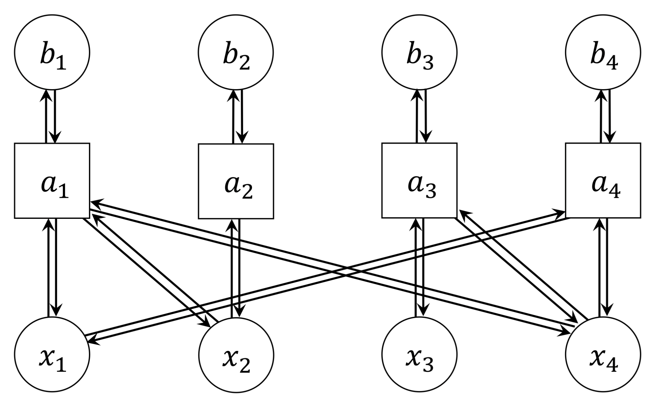
2.1. Factor Graph Representation of a Linear Equation System

A Factor Graph (FG) is an undirected bipartite Bayesian network being composed of variable nodes, which represent random variables, and factor nodes, which model functional dependencies between them [16]. In our case, we make use of a FG to model the objective function p ( x ) in (5) which can be interpreted as a PDF. Here, x i , i = 1 , , N play the role of random variables as well as the elements of vector b . The linear equations expressed by rows of matrix A represent functional dependencies of these variables. Because of the nicely factorized form of p ( x ) in (5), the construction of the FG is straightforward.
Our FG G = ( N , E ) is defined by its set of nodes N and its set of edges E . The set of nodes N = F V can be decomposed into a set of factor nodes F = { a 1 , a 2 , a N } and a set of variable nodes V = { x 1 , x 2 , , x N , b 1 , b 2 , , b N } with cardinality | F | = N and | V | = 2 N . Note that every element x i basically corresponds to a variable node x i and every element b i to b i , respectively. Every factor node a i can be associated with the ith row of matrix A , i.e., the ith equation of our LES.
The connectivity of G and its edges E heavily depends on the structure of matrix A . Note that in general edges in an FG are undirected [16]. Nevertheless, here we consider the edges to possess a direction, and therefore, we define for every connection between two nodes in the FG two edges—one for each direction. This notation will pay off later on when deriving the Message Passing Algorithm.
The set of edges E = E b E A can be decomposed into a set E b with edges independent of A and a set E A dependent on A . Due to the fact that every ith equation of the LES contains the ith element of vector b , there is always a connection between b i and a i forming the set:
E b = { ( b i , a i ) | i { 1 , , N } } { ( a i , b i ) | i { 1 , , N } } .
The other edges in E A depend on A in the form:
E A = { ( x i , a j ) | i { 1 , , N } , j { 1 , , N } , A j , i 0 } { ( a j , x i ) | i { 1 , , N } , j { 1 , , N } , A j , i 0 } .
For a better understanding, let us construct the graph for a simplified example. Here, matrix A and vector b are arbitrarily chosen as following with resulting x for N = 4 :
A = 2 1 0 3 0 2 0 0 0 0 4 2 1 0 0 2 , b = 6 2 2 1 x = 7 1 1 3 .
The corresponding FG for the example is shown in Figure 1.

2.2. Message Passing Algorithm

The purpose of the FG defined in the previous section is to derive a Message Passing Algorithm that delivers the marginal distributions p i ( x i ) . Note again: as soon as we find the maximum of each marginal distribution, we found the vector x that solves the LES. We make use of Belief Propagation [2], sometimes called Sum-Product Algorithm. The algorithm computes marginal distributions of variable nodes x i by exchanging messages between the nodes along the graph’s edges. In our case of GaBP, all messages in the graph are Gaussian-shaped PDFs [10]. As such messages (in the graph) are always fully defined by their mean and precision (i.e., inverse variance). In cases, where a factor graph is loop-free, all messages have to be sent only once in order to calculate the exact marginal distributions [16]. Unfortunately for a general LES, it is not guaranteed that no loops exist. For example, in the graph in Figure 1, the edges ( a 1 , x 4 ) , ( x 4 , a 4 ) , ( a 4 , x 1 ) , ( x 1 , a 1 ) form a closed loop. So, it is not ensured that the algorithm provides the true marginal distributions. Nevertheless, in many practical cases, it is known that loopy Belief Propagation [17], where messages are transmitted several times in the graph, does converge to an approximate solution [18].
Now, let’s have a look at the algorithm in more detail. In the graph, there are two types of messages: (i) messages sent from a factor node to a variable node m f i v j and (ii) messages from a variable node to a factor node m v i f j with f i F and v j V . The Sum-Product Algorithm provides us with general update rules on how to calculate these messages [4]:
m v i f k = f j I i , k m f j v i ,
with the set I i , k = { f j | j , ( f j , v i ) E , j k } . In other words: The outgoing message from a variable node to a factor node f k is the product of all incoming messages to variable node v i except the message coming from f k .
The second update rule is:
m f k v i = g k ( K i , k , v i ) v j K i , k m v j f k d K i , k ,
with the set K i , k = { v j | j , ( v j , f k ) E , j i } . Here, g k is a function that describes the relation of all variables of variable nodes in K i , k and v i according to the factor node f k . Further, the notation d K i , k indicates the integral over all variables of the variable nodes in K i , k .
Let’s apply these update rules to our problem of a LES. In our GaBP case, the update in Equation (11) turns out to be a simple multiplication of Gaussian functions, which is a Gaussian again. In our case, there exist two different types of variable nodes: x i and b i with the following update rules for x i :
m x i a k G ( x i | μ x i a k , τ x i a k 1 ) , τ x i a k = a j I i , k τ a j x i , μ x i a k = 1 τ x i a k a j I i , k μ a j x i τ a j x i ,
with I i , k = { a j | j , ( a j , x i ) E , j k } for this particular case. Here G denotes a Gaussian function and all μ denote means and all τ precisions, respectively.
For messages from b i , there is no update rule, since b is given. Actually, the graph described in the previous section contains additional factor nodes that constrain the variable nodes b i as depicted in Figure 2. However, commonly in literature, these additional factor nodes are neglected [4] for simplicity. The outgoing messages from b i boil down to:
m b i a k G ( b i | b ^ i , τ b 1 ) ,
with the actual scalar values b ^ i of the given vector b i and a predefined precision τ b 1 . We set this precision to a high value ( 10 5 ) modeling our trust in the correctness of vector b i .
Applying update rule (12) to our problem is a little bit more involved. Let’s first consider message m a k b i . While it is possible to formally define this message, it is practically irrelevant for the algorithm. Therefore, we are not going to derive it. The messages to x i are required and, after some algebra, result in:
m a k x i G ( x i | μ a k x i , τ a k x i 1 ) , τ a k x i = A k , i 2 ( b ^ k 2 τ b 1 + x j K i , k A k , j 2 τ x j a k 1 ) 1 , μ a k x i = 1 A k , i ( b ^ k + x j K i , k A k , j μ x j a k ) ,
with set K i , k = { x j | j , ( x j , a k ) E , j i } for this particular case. (Note: here we used τ s )
As can be seen from the equations, outgoing messages from a node are always functions of the incoming messages to the specific node. In one iteration of our Message Passing algorithm, each message in the graph is calculated once in a specific order. The order we are going to describe later on. If for an update, a message is required, that has not been calculated for the current iteration, we make use of the results from the previous iteration. This approach requires the initialization of messages for the first iteration. We choose a random mean μ x i a k and μ a k x i from a uniform distribution [ 1 , 1 ] . The precision of a message can be interpreted as the certainty of the corresponding variable. Therefore, we initialize τ x i a k and τ a k x i with low values accounting for the fact that we do not know the variables at the beginning. Thus, the initial messages essentially correspond to wide Gaussian distributions. Note that the messages m b i a k are always the same for every iteration. As such they are calculated once at the beginning but do not require any update or initialization.
The actual marginals we are looking for are given as:
p i ( x i ) = a j J i m a j x i G ( x i | μ i , τ i 1 ) , τ i = a j J i τ a j x i , μ i = 1 τ i a j J i μ a j x i τ a j x i ,
with the set J i = { a j | j , ( a j , x i ) E } . Once again, note that μ i are the maxima of the marginals and the solution to our LES. Since our graph contains loops, these marginals are only approximations of the actual distributions. By iteratively exchanging all messages in the graph the approximations converge to the true marginals under certain conditions, which we are going to evaluate in the result Section 4.
As a last ingredient of the algorithm, we need a schedule to calculate the messages. A common approach is to calculate the messages in random order [16]. However, this might not be the most efficient way. For example, in [19] a more efficient scheduler is proposed taking into account the information flow in the graph. However, scheduling is not the main focus of this paper and we stick to the common, yet less efficient, random order for calculating the messages. In our case the scheduler is asynchronous, and it updates all existing messages in one iteration before updating the same message in the next iteration. For updating a message in a certain iteration, we make use of an already updated version of the required messages.
Finally, at this point let us remark that a termination or convergence criterion of the algorithm is required. The decision on that is up to the particular application. In our studies in Section 4, we use a fix number of Message Passing iterations.

3. Hardware Implementation in a FPGA

The main motivation of our paper is to speed up GaBP and thereby solving the LES by implementing the algorithm in hardware on a FPGA. We achieve this by the design of specialized co-processors, taking care of the most intensive, recurring computations. In particular, we outsource the computation of the messages in Equations (13) and (15) to two types of dedicated co-processors. Multiple co-processors of these types can calculate messages in parallel and speed up the algorithm while at the same time relieving the CPU.
Our implementation is designed for a SoPC. The SoPC combines a standalone processing system integrated with programmable logic on a single die. The programmable logic, which is basically a FPGA, consists mostly of configurable logic fabric. On this fabric, the digital hardware defined by a Hardware Description Language can be physically implemented. For our evaluation, we have chosen SoPCs running chip-sets based on the Zynq-architecture by Xilinx [20]. Here the processing system is an ARM processor with all components required for an independent, CPU-driven system. The programmable logic and processing system are connected via a set of interconnecting bus systems, allowing data transfer between hardware implementations in the logic fabric and the CPU system [21].
In the next two subsections, we are going to describe the design of the co-processors and explain their interfaces and memory access.

3.1. Dedicated Co-Processors for Message Passing

We employ two different types of co-processors in our hardware design: One is taking care of calculating messages m x i a k according to Equation (13). Therefore, we label this type of co-processor C x a . The other co-processors labeled C a x calculates messages m a k x i according to Equation (15), respectively. More precisely, the co-processors calculate the mean and precision of corresponding messages simultaneously. Recap that a message is fully defined by its mean and precision.

3.1.1. Co-Processor C x a

Co-processor C x a is shown in Figure 3a. As can be seen, the mean and precision of incoming messages propagate through floating-point computation hardware blocks in order to calculate the outgoing message according to Equation (13).
The incoming messages required to calculate the outgoing messages m x i a k are fed to the co-processor in the form of 64-bit packages via an AXI4-stream slave interface [21]. Here, the upper 32 bits of a package encode the mean in form of 32-bit floating-point numbers, where the lower 32 bits encode the precision, respectively. Figure 4a illustrates this protocol. The co-processor puts out the resulting messages in a similar format.
First, a broadcaster block at the slave port of C x a splits the 64-bit incoming packages into a 32-bit floating-point mean μ and a 32-bit floating-point precision τ . Another broadcaster doubles the precision τ . One path of τ is accumulated in a floating-point accumulator block. These blocks are automatically reset after receiving input with a flag indicating the final package of the stream. The accumulated result is basically the precision of our outgoing message according to (13). It is extracted by the finalize-accumulation block and again doubled, where one path already goes to the combiner block for assembling the final package for the outgoing message.
Let’s go back to the second τ path. It joins the μ path in a floating-point multiplication block, where the precision τ and μ are multiplied as required by Equation (13) for the calculation of the outgoing mean. These products are accumulated in another floating-point accumulator block, and a finalize-accumulation block extracts the result. The accumulated products join the accumulated precisions in a floating-point division block, where finally the mean of the outgoing message is calculated. The 32-bit mean and the 32-bit precision are assembled in the combiner block to a 64-bit package, representing the message m x i a k to which the co-processor is dedicated.
Remark: The broadcasters, floating-point accumulators, and floating-point multiplication as well as divisions are Intellectual Property (IPs) provided by Vivado [22]. They allow fast floating-point operations in hardware, making use of specialized hardware for floating-point arithmetic available on the PL and optimized for latency and speed [22].

3.1.2. Co-Processor C a x

The second type of co-processor, C a x , calculates the messages m a k x i according to Equation (15). The co-processor is illustrated in Figure 3b. The messages, more precisely the precision τ a k x i and mean μ a k x i , are calculated based on incoming messages to factor node a i . However, they do not only depend on the incoming messages, but also on the linear function represented by factor node a k , i.e., the k-th equation of our LES (1). Essentially, the co-processor needs to know all non-zero elements of the k-th row of A as well as the k-th entry in vector b of Equation (1). To feed all required information to the co-processor C a x , we deploy the protocol shown in Figure 4b for the AXI input stream. Here again, we are constrained by the 64-bit package size.
In the co-processor, first, a switch routes all incoming packages as shown in Figure 3b according to the order of arrival. The first package, containing A k , i two times as 32-bit floating-point values, goes to path 1. Every even package is routed to path 2. They contain the mean (upper 32 bits) and precision (lower 32 bits) of the incoming message to factor node a k from variable nodes x j and node b k . The odd packages except the first one go to path 3 and contain the non-zero coefficient of the linear equation k, i.e., A k , j . Again, the value is contained two times as a 32-bit floating-point value to match the 64-bit package size. Note that the coefficient for b is actually 1 , as also illustrated in the example in Figure 4b.
Further, in the co-processor, the inputs are propagated and processed as follows: From path 1, A k , i is extracted by a broadcaster block twice, where one is squared, and one is negated (multiplied by 1 ) in dedicated blocks. In path 2, means μ a k and precisions τ a k are separated by a broadcaster. The means are multiplied by the coefficients A k , j extracted from path 3. The resulting products are summed up by an accumulator block, and the final sum is extracted by a finalize-accumulation block. The sum is divided by the negative A k , i in a division block, which already provides us the mean μ a k x i of the outgoing message.
Simultaneously the co-processor calculates the precision τ a k x i . Therefore, all A k , j are squared and divided by all τ a k . Again, these values are summed up by an accumulator and finalize-accumulation block. Dividing the sum by squared A k , j provides the final precision τ a k x i which is combined with the mean μ a k x i to a 64-bit package in a combiner block before it is sent out to the AXI stream.
It is important to note that all hardware blocks in both kinds of co-processors, and therefore the co-processors themselves are designed for maximal latency. This means that it takes multiple clock cycles after receiving a valid input until a valid output is ready at the hardware block. Yet, at every clock cycle, a new set of input data can be accepted by such hardware block. Further, floating-point blocks with two inputs work in a blocking manner. So, they require a pair of valid input data. Due to different propagation path lengths in the co-processor, this could lead to congestion. We avoid this by FIFO-buffer blocks that can store data until the second input is valid, too. These blocks are not displayed in Figure 3 for the sake of readability.

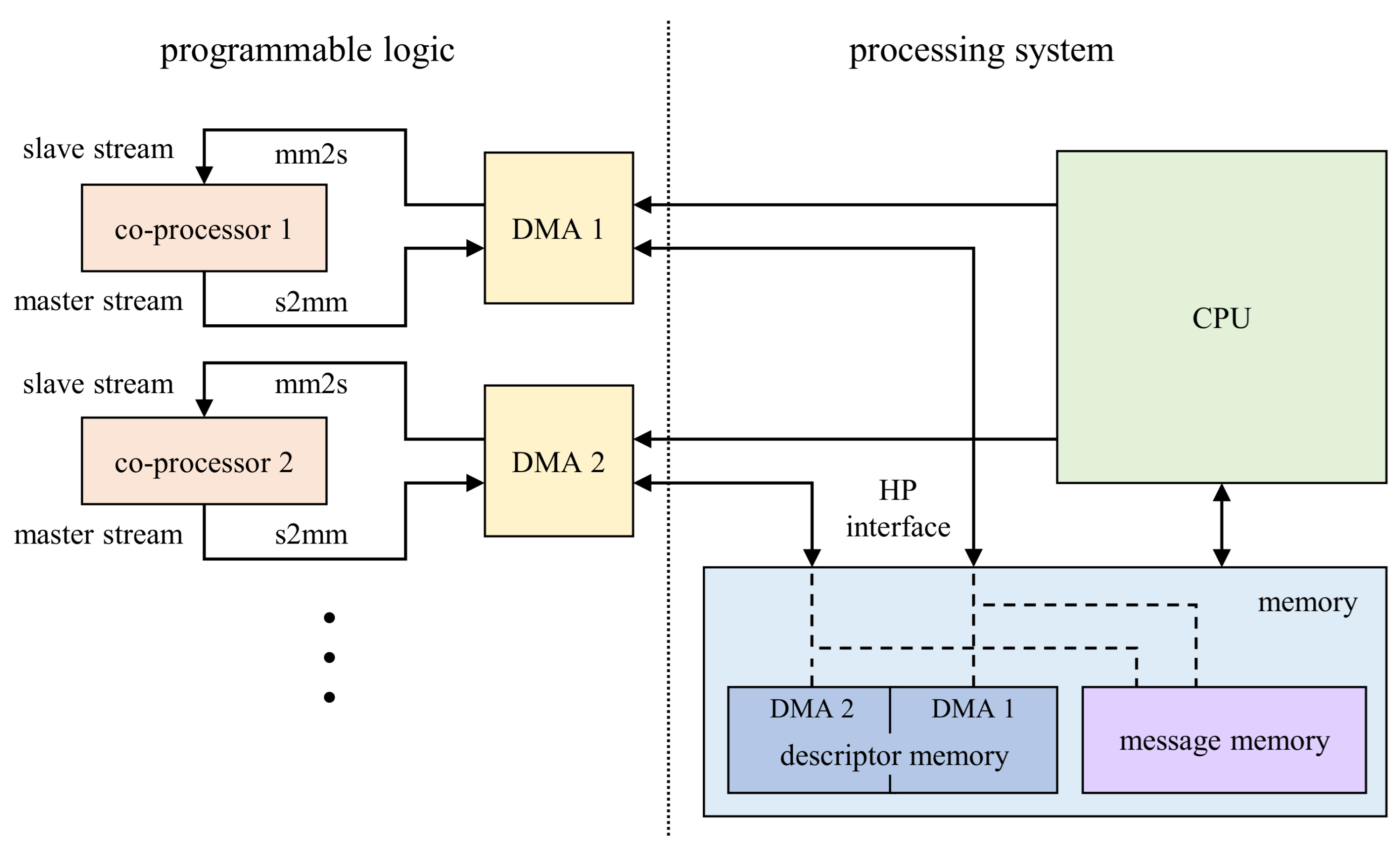
3.2. Interfaces and Memory Access of the Co-Processors

As we have seen in the previous subsection, the co-processors need input data provided by an AXI stream. This subsection is going to explain how the data are streamed to the co-processors and how the co-processors are connected to the processing system of the SoPC. It is also illustrated in Figure 5.
Every co-processor, either of type C a x or C x a is implemented in the programmable logic of the SoPC and equipped with a separate DMA module. DMAs are able to read and write data from the processing system’s memory via a high-performance interface [23]. In addition, they are directly connected to the CPU by a general-purpose interface that allows to start and configure the DMAs. Apart from that, in our setup they are working independently of the CPU in a so-called scatter-gather mode [23]. In this configuration, each DMA requires two sets of descriptors stored in the processing system’s memory:
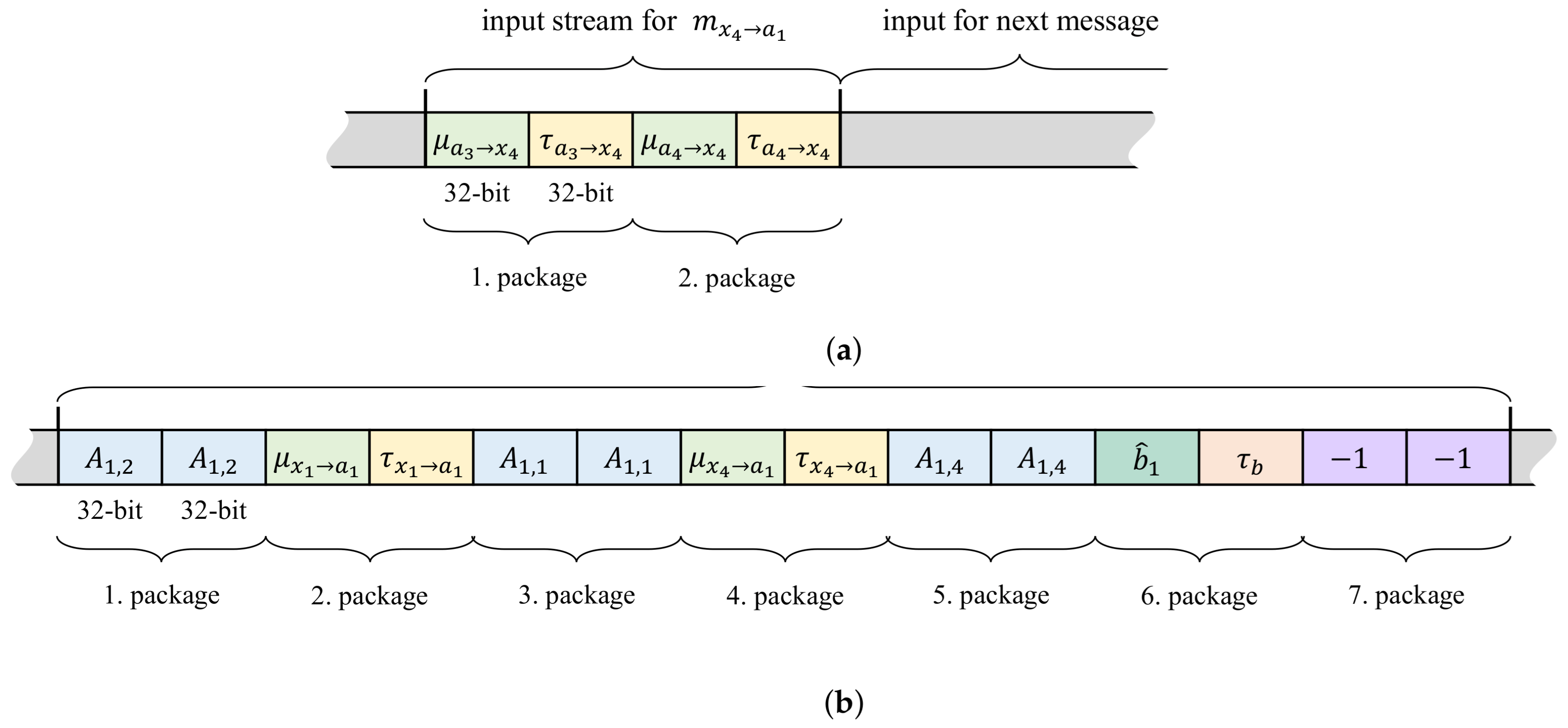
  • Memory Mapped to Stream (mm2s) descriptors contain the addresses in memory where to fetch data from as well as the number of bytes to fetch. The fetched data is streamed to the hardware co-processor connected with an AXI4-Stream interface to the DMA.
  • Stream to Memory Mapped (s2mm) descriptors on the other hand contain the addresses in memory where to write data to and the data length. The data is coming to the DMA also via an AXI4-Stream interface.
In other words, both types of descriptors are basically lists of addresses where to read from or where to write to. Note that both transmissions mm2s and s2mm are handled independently from each other by the DMA.
In our proposed design all messages, i.e., their mean and precision, are stored in allocated memory (message memory) on the processing system along with the entries of matrix A and vector b . The descriptors of the DMA are compiled by the CPU and stored in dedicated memory (descriptor memory) of the processing system accessible by the DMAs’ scatter-gather engines. These descriptors define the order in which mean, precision, and coefficients are streamed to the co-processors. As such, they have to match our chosen protocol described by Figure 4 of the input streams. With the input data in the right order, the co-processor computes a new message, i.e., mean and precision. The connected DMA receives this message from the master interface of the co-processor and writes it back to the appropriate location in message memory according to its current s2mm descriptor. In this way, all messages stored in the processing system’s memory are subsequently updated by the co-processors and DMAs without CPU interventions.
Remark: In general, a DMA processes the descriptors once and stops. After that, the DMA would need to be restarted by the CPU. However, DMAs can also operate in a “cyclic mode” [23]. In this mode, the DMA loops through the descriptors once and starts again from the beginning ad infinitum. This mode is especially interesting for the computation in our algorithm since messages have to be computed multiple times until convergence.

4. Evaluation

In this section we are going to evaluate our proposed approach for solving LES on dedicated hardware. We first present the evaluation boards used in our experiments, then we explain how we generated different LESs for our evaluation purpose. Finally, we show the results of our evaluation and compare the performance of our approach to a state-of-the-art solver.

4.1. Deployed SoPC Boards

In our evaluation we make use of two different SoPC boards: one being the PYNQ-Z1 [24] and the other one the Zynq UltraScale+ ZCU104 [21] (pictured in Figure 6). Both boards share the same architectural foundation. They are equipped with chipsets based on the Zynq-architecture [20]. On both SoPC boards, the development environment “Python Productivity for Zynq” is available. This allows executing python code on the processor and making use of existing libraries. Furthermore, programmable hardware that is synthesized in the programmable logic can be incorporated in the execution [24]. The two evaluation boards differ in computational power and in the available hardware resources. The more affordably priced PYNQ-Z1’s processing system is equipped with a 650 MHz dual core ARM processor and 512 MB of DDR3 RAM. The programmable hardware is connected to the processing system with four high performance ports. The Zynq UltraScale+ ZCU104 on the other hand comes with a processing system driven by a 1.3 GHz quad core ARM processor and 4 GB of fast DDR4 RAM [21]. The Zynq UltraScale+ ZCU104 has a larger amount of programmable hardware resources available in comparison to the PYNQ Z1. It can be accessed through a total of six high performance ports. So, it can host six co-processors for message passing in contrast to only four on the PYNQ-Z1.
The utilization of available hardware on the programmable logic is illustrated in Figure 7. The figure shows the required space of the implementation of the co-processor on the FPGA for both boards in (a) and (b). Note that the regions marked as “other” are mostly used by the DMAs. As can be seen, also from the quantitative utilization in (c) and (d), the available hardware resources are not completely exploited. Therefore, we would like to remark that the limiting factor in our approach is the number of available high-performance interfaces (and their bandwidth).
The clock speed for the programmable logic has been set to 100 MHz for both boards in our implementation. Presumably, the clock speed could be increased. (Current Worst Pulse Width Slack: 3.75 ns PYNQ-Z1 and 3.50 ns Zynq UltraScale). A higher frequency would also speed up the algorithm.

4.2. Evaluation Data Sets
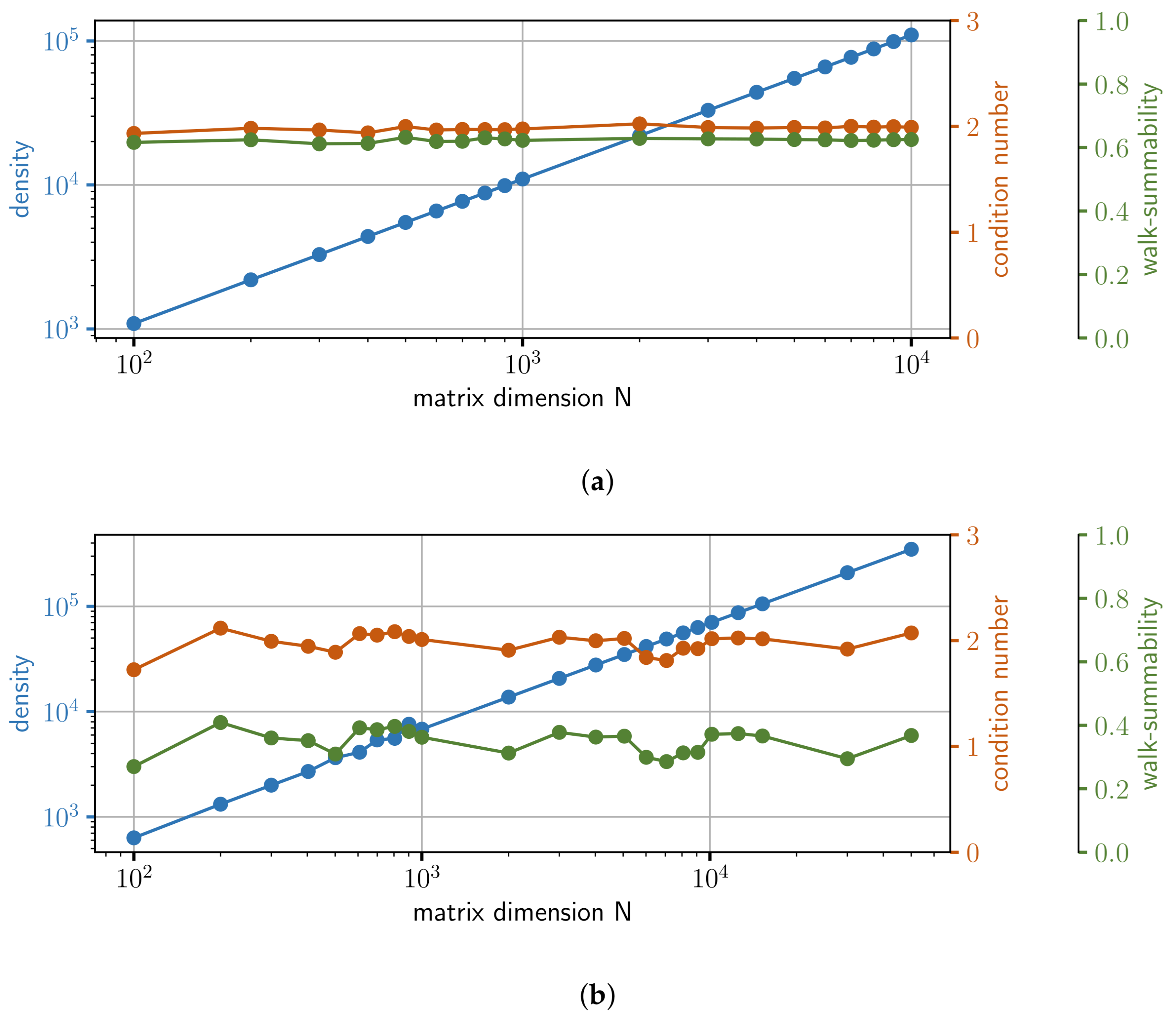
In order to evaluate our approach, we generated different sets of LESs. We solved these LESs with our GaBP algorithm on the hardware mentioned above. In our studies, we analyze the quality of the solution and the time it took to compute the solution with respect to different properties of the LES. The first property is the density of matrix A , which is the number of elements in A that are not zero. Second, we have a look at the condition number of A . We would expect that a LES with a condition number closer to 1 would be easier to solve. Last but not least, we consider the so-called walk-summability condition [14,15]. Unfortunately, it is not guaranteed that the GaBP converges for an arbitrary LES. However, it has been shown that the algorithm converges for ω < 1 [15] with
ω = ρ I D 1 / 2 A D 1 / 2 ,
and ρ being the spectral radius and D the diagonal matrix of A [12]. In the following, we refer to ω as the “walk-summability” of A . We make sure that for all our LESs the walk-summability is below 1. Note that this is a sufficient condition, but it is not a necessary condition for convergence.
We investigate four different sets of LESs with different matrices A and vectors b that we designed in the following way:
  • Random LESs: We generate A and b for different dimensions N, i.e., number of equations. Here N covers the whole list [100, 200, 300, 400, 500, 600, 700, 800, 900, 1000, 2000, 3000, 4000, 5000, 6000, 7000, 8000, 9000, 10,000]. The entries in the vector b are sampled from a random uniform distribution between 1 and 1. Matrix A is designed in a way so that it is sparse and diagonal dominant. The density, i.e., the number of elements that are not zeros, is chosen to be 10 N , where the location of non-zero elements is random (Here we make use of the scipy library [25], namely the function “scipy.sparse.random”). The non-zero entries are also sampled from a random uniform distribution between 1 and 1. In addition, we add the value 8 to all diagonal elements of the random sparse matrix to get our final matrix A . The main properties of the matrices in this set of LESs are depicted in Figure 8a, where each dot on a line represents one matrix. As can be seen, the condition number, as well as the walk-summability is roughly constant, while the density increases linearly with dimension N. This set contains in total 19 LESs.
  • Finite Element Method (FEM) LESs: For the second set, we consider the Poisson PDE x ( t ) = b ( t ) with t Ω and the domain Ω = [ 0 , 1 ] x [ 0 , 1 ] with boundary condition x ( t ) = 0 , t Γ on border Γ of domain Ω . We numerically approximate this variational problem by FEM and Lagrange elements of order one. FEM turns our problem into a LES A x = b . However, this approach requires discretizing the domain Ω by a finite number of elements spanning a mesh. The number of nodes of this mesh defines dimension N of our LES. A higher number of nodes and thus a better resolution of the numerical approximation results in a higher dimension N. Before we solve the LES on our hardware, we use an incomplete LU preconditioner [26]. The preconditioner is parameterized in a sub-optimal way. This is on purpose to challenge our solver and to make sure that we do not accidentally solve a linear system where the matrix A is the identity matrix, or very close to it. (This would be a trivial problem.) Preconditioning is also a common approach for standard numerical solvers of LES [26]. The main properties of the matrices in this set are depicted in Figure 8b. We parametrize the preconditioner so that the condition number and walk-summability are roughly constant. Nevertheless, there is some variation. We used different meshes in the FEM with different resolutions. Thus, the set contains in total 23 LESs with different dimensions N. All entries in vector b are set to zero, except the one entry corresponding to the point in the middle of the domain. This entry is set to 1.
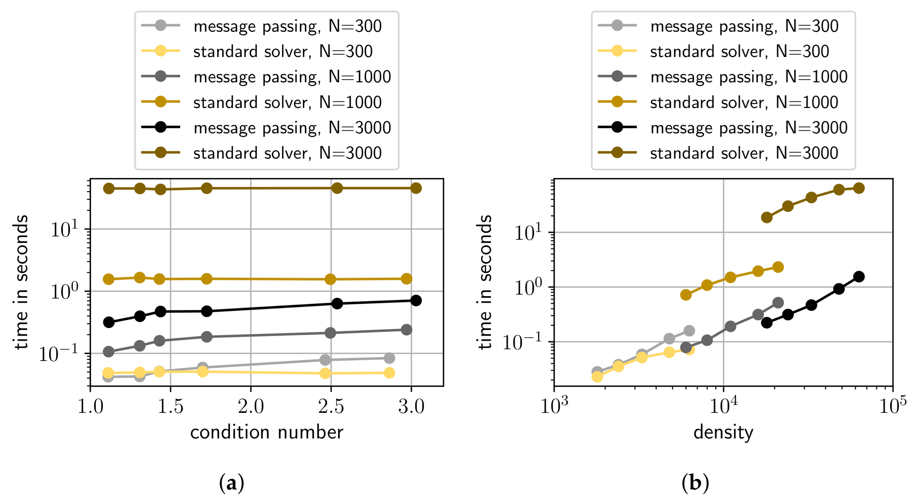
  • Constant density LESs: This set of LESs is generated in a similar way as the Random LESs, however, only for dimensions N {300, 1000, 3000}. The density of matrix A is again 10 N . In contrast to the Random LESs, we add different values to the diagonal elements of the randomly generated sparse matrices (5.1, 6, 10, 15, 20, 50). The properties of matrices are shown in Figure 9a. As can be seen, in this set, for a given dimension N, the density is constant for different condition numbers. Entries in vector b are again sampled from a random uniform distribution between 1 and 1.
  • Constant condition number LESs: Again this set is generated similar to the Random LESs, but only for dimensions N { 300, 1000, 3000}. This time, we generate matrices A with different densities, namely γ N , with γ { 6, 10, 15, 20, 50}. We also add γ to the diagonal elements of A resulting in approximately constant condition numbers for different densities. This dependency is also depicted in Figure 9b. Entries in vector b are again sampled from a random uniform distribution between 1 and 1.

4.3. Performance of GaBP on a SoPC

In order to evaluate the performance of our approach, we need a benchmark that we can compare to. Here, we make use of the sparse linear solver of the scipy python library [25] (namely the function “scipy.sparse.linalg.spsolve”). We use this solver to solve our different LESs, and its solution we denote as x s l s . The quality of our approach we measure as the discrepancy (or error) between our solution x and x s l s as
e = x x s l s L 1 x s l s L 1 .
Apart from that we also measure the time it took the state-of-the-art solver and our approach to solve the LES.
Let us remark that for direct comparison, we run the state-of-the-art solver on the ARM processing system of the respective SoPC board. Therefore, the times on the PYNQ-Z1 are much higher due to the less powerful CPU. Also, the 512 MB RAM on the PYNQ-Z1 constrains us to only solve LESs with dimension N < 8000 . In addition, we also measured the time that the standard sparse solver required to solve the LES on a Workstation (Intel(R) Core(TM) i7-3820 CPU @ 3.60 GHz with 32 GiB DDR3 System Memory). Of course, this power-full device requires expectably less time to solve the LES. However, in our focused applications in mobile robotics, it is often impossible to equip a robot with a heavy, high-power consuming workstation.
Let us first look at the result for the set of Random LESs. The results for the Zynq UltraScale board are shown in Figure 10 and the result for the PYNQ-Z1 in Figure 11. As can be seen from Figure 10a and Figure 11a, the message passing algorithm achieves a very good approximation of x after only a few iterations. On both boards, an error below 10 6 is already reached after approximately 10 to 15 iterations. Remarkably, the number of iterations is independent of the dimension N of the LES. As expected, the error and convergence of the algorithm are very similar on both boards, since the algorithm is implemented in the same way on both boards; despite the fact that on the Zynq UltraScale six co-processors are running in parallel, where on the PYNQ-Z1 only four.
The required times to solve the LES are depicted in Figure 10b and Figure 11b. The orange curves show the time the standard scipy solver required to solve the equation. The solid line represents the standard solver running onboard on the ARM processing system. The dotted line shows the times required by the workstation for comparison. The solid black lines indicate the time our approach needed to achieve an approximation of x with an error below 10 5 . The dashed lines represent the time of a single Message Passing iteration. For our evaluation purpose, we start and stop the DMAs for every message passing iteration, in order to calculate intermediate results and analyze convergence. This overhead of starting and stopping DMAs is represented by the dotted lines. This time can be saved in case the DMAs operate in a scatter-gather “cyclic mode”. As can be seen from both plots, our approach scales better than the standard solver with respect to dimension N on both boards. Thus, for LESs with N > 400 , our approach outperforms the standard solver. The benefit gets bigger with increasing dimension N. Even compared to the workstation, our approach is faster for N > 1000 . For the required time of the Message Passing Algorithm, the two boards differ. For example, the LES with N = 1000 took 0.426 s on the PYNQ-Z1 with four co-processors and 0.185 s on the Zynq UltraScale with six co-processors. This indicates that hardware, allowing us to employ more co-processors, may further speed up our approach.
Next, let’s look at the set of FEM LESs. The results are shown in Figure 12 for the Zynq UltraScale board and in Figure 13 for the PYNQ-Z1 board. Again the plots in (a) show the errors of the Message Passing solutions compared to the standard solver’s solutions for different numbers of message passing iterations. As can be seen, the convergence is quite fast, similar to the set of Random LES. Within 20 iterations the algorithm accomplishes results with errors below 10 6 for both boards. However, it is noticeable that for LESs between dimension 400 and 1000 the error curves show irregularities. We blame our preconditioner for this effect. The condition number for the FEM LESs shows some variation (see Figure 8) with respect to the different LESs. This seems to affect the convergence of our algorithm. (We are going to investigate this effect further down.)
The time of our approach compared to the state-of-the-art solver is depicted in Figure 12b and Figure 13b for the FEM LESs. The solid black line again shows the time the algorithm needs to get a solution better than 10 5 . The dashed line indicates the time of one message passing iteration and the dotted line the DMA overhead. It appears that for this type of LES the standard solver is almost always faster. However, the Message Passing Algorithm scales better so that for a LES with dimension N > 15 , 000 our approach is faster compared to the standard solver on the Zynq UltraScale ARM processing system. Unfortunately, the memory (4 GB on the Zynq UltraScale and 512 MB on the PYNQ-Z1) limits the maximum dimension we can solve on the chosen boards so that we cannot profit from the better performance on higher dimensions. Thus, our approach never outperforms the workstation for the FEM LESs set. Hopefully, in the future affordable boards with more memory become available. Then, our approach can pay off for larger LESs of this type. It is also notable that the irregularities in the convergence plots in (a) are reflected by the time our approach needs to solve the LES, but also in the times of the standard solver. As mentioned, this may indicate a bad condition of certain LESs in this set.
A full convergence analysis of GaBP is not in the scope of this paper. (see for example [15,27,28] on this topic) Nevertheless, we would like to give the reader some insight what are favorable properties of a LES in order to be solved efficiently by our Message Passing Algorithm. To this end, Figure 14 and Figure 15 show the performance of our approach for the sets of LESs with a constant condition number and a constant density. While Figure 14 shows the required time to solve the LES in comparison to the standard solver for different dimensions, Figure 15 shows exemplarily the convergence of the algorithm only for dimension N = 1000 .
As can be seen from Figure 15a, the error of a solution after a particular number of iterations increases with increasing condition number. Also, a higher condition number causes a slightly higher computation time as shown in Figure 14a. Even though this effect is quite low for the considered range of condition numbers, one can say that a better condition number, i.e., closer to 1, is of advantage for our approach.
In contrast, the impact of a higher matrix density on the computation time is much higher as can be seen from Figure 14a. The computation time increases not only for our approach but also for the standard solver. If we in addition look at the convergence for dimension N = 1000 and different densities in Figure 15b, we can see that convergence, however, is even slightly better for higher densities. This indicates that the Message Passing Algorithm does not need more iterations to converge for higher densities. Thus, the increasing computation time is solely attributable to the higher number of messages that need to be calculated within one iteration. Recap that the number of messages is proportional to the number of entries in matrix A , i.e., the density. It is also notable in Figure 14b that the computation time of the standard solver jumps for increasing dimension N of the LES. This is not the case for GaBP. Surprisingly, the time of the Message Passing Algorithm to converge is lower for higher dimensions N compared to LESs with lower dimensions but the same density. Here, the effect may be caused by a convergence within fewer iterations, which we already observed in Figure 15b.

5. Conclusions and Remarks

To sum up: In this paper, we make use of GaBP to solve LESs. More precisely, we reformulate our LESs as Gaussian PDFs, which we model by a Factor Graph (FG). The FG is the foundation of a Message Passing Algorithm we derived according to GaBP. The algorithm provides us with approximations of the marginal distributions of the PDF. Essentially, the maxima of these marginals are the solutions to our LESs. The algorithm requires to compute messages according to simple update rules. Even though, the updates are simple algebraic computations, a lot of messages need to be calculated. We make use of a SoPC, where we designed dedicated co-processors for the programmable logic taking care of the message updates. By outsourcing the message updates, the CPU is relieved. In this paper, we have shown that this approach achieves good approximations of the solution for certain LESs. In addition, the performance with respect to the computation time of our approach has turned out to scale better compared to a state-of-the-art sparse linear solver.
Here, we would like to remark that even for LESs, where the Message Passing Algorithm shows similar speed compared to a standard solver, our approach is of advantage, since the CPU is not occupied and can be used for other tasks.
It is also worth mentioning that the Message Passing Algorithm delivers the variances of the marginals as a side product for free. These variances are of interest in some applications like uncertainty-driven robotic exploration strategies [1,29]. A classical approach would require calculating the inverse of matrix A to obtain these variances. The calculation of the inverse, however, is much more computationally expensive compared to just solving the LES. This can be considered as another advantage of the GaBP approach.
Further, GaBP can be easily extended to a Bayesian framework, which allows the introduction of prior assumptions that can act as a kind of regularization on the LES. For example, in [30], a similar Message Passing Algorithm has been employed with a sparsity inducing prior based on Sparse Bayesian Learning techniques [31].
We would also like to remark that the limiting factor in our evaluation was the low amount of memory on the deployed evaluation boards (4 GB on the Zynq UltraScale). The memory limits the number of messages and DMA descriptors, and thus, the maximum dimension of LESs, which can be handled. In the future, there might come up more powerful, low-priced SoPCs allowing us to solve even larger LES with our approach.
The second limiting factor in our approach is the number of high-performance interfaces between programmable logic and the processing system. In our design, each co-processor requires one DMA that is attached to a single high-performance interface to get memory access. In general, it would be possible to attach multiple DMAs to a single high-performance interface; or to attach multiple co-processors to each DMA. The latter would require us to change our protocol in Section 3.1. However, the high-performance interfaces provide a theoretical bandwidth of 1200 MB/s [32] at a clock frequency of 150 MHz (in both directions). This equals a theoretical bandwidth of 800 MB/s at the clock frequency of 100 MHz in our design. Each of the co-processors is able to process input data with the same bandwidth of 64 bit × 100 MHz = 800 MB/s. Thus, there is no improvement by running multiple co-processors per high-performance interface, since the bottleneck is the limited bandwidth of the interface. With increased clock frequency, however, both the bandwidth of the high-performance interfaces and the co-processors can be increased. In addition, more high-performance interfaces between programmable logic and the processing system would enable more co-processors to run in parallel.
At this point, it is also important to remark the main drawback of GaBP for solving LESs: For general LESs, it is not guaranteed that the algorithm converges. In this paper, we only investigated diagonal dominant matrices that fulfill the walk-summability condition [14,15]. In general, our approach cannot be applied to all types of LES. However, for some applications, like LESs arising from numerical approximations of PDEs, it is suitable. Thus, it may support model-based robotic exploration strategies in the future.

Author Contributions

Conceptualization, T.W.; methodology, J.S., T.W.; software, J.S.; validation, J.S., T.W.; formal analysis, J.S., T.W.; investigation, J.S., T.W.; resources, J.S., T.W.; data curation, J.S.; writing—original draft preparation, J.S., T.W.; writing—review and editing, J.S., T.W.; visualization, J.S., T.W.; supervision, T.W.; project administration, T.W.; funding acquisition, T.W. All authors have read and agreed to the published version of the manuscript.

Funding

This research received no external funding.

Conflicts of Interest

The authors declare no conflict of interest.

Abbreviations

The following abbreviations are used in this manuscript:
PDEPartial Differential Equation
FPGAField-Programmable Gate Array
LESLinear Equation System
GaBPGaussian Belief Propagation
SoPCSystem on a Programmable Chip
DMADirect Memory Access
FEMFinite Element Method
FDMFinite Difference Method
PDFProbability Density Function
FGFactor Graph
CPUCentral Processing Unit
IPIntellectual Property

References

  1. Wiedemann, T.; Manss, C.; Shutin, D.; Lilienthal, A.J.; Karolj, V.; Viseras, A. Probabilistic modeling of gas diffusion with partial differential equations for multi-robot exploration and gas source localization. In Proceedings of the European Conference on Mobile Robots (ECMR), Paris, France, 6–8 September 2017; pp. 1–7. [Google Scholar] [CrossRef]
  2. Pearl, J. Probabilistic Reasoning in Intelligent Systems; Morgan Kaufmann Publishers: San Francisco, CA, USA, 1988. [Google Scholar]
  3. Frey, B.J.; Kschischang, F.R. Probability Propagation and Iterative Decoding. In Proceedings of the 34th Allerton Conference on Communications, Control and Computing, Champaign-Urbana, IL, USA, 2–4 October 1996. [Google Scholar]
  4. Loeliger, H.A. An Introduction to Factor Graphs. IEEE Signal Process. Mag. 2004, 21, 28–41. [Google Scholar] [CrossRef] [Green Version]
  5. Oommen, M.S.; Ravishankar, S. FPGA implementation of an advanced encoding and decoding architecture of polar codes. In Proceedings of the 2015 International Conference on VLSI Systems, Architecture, Technology and Applications, VLSI-SATA 2015, Bengaluru, India, 8–10 January 2015; pp. 1–6. [Google Scholar] [CrossRef]
  6. Yang, Q.; Wang, L.; Yang, R.; Stewénius, H.; Nistér, D. Stereo matching with color-weighted correlation, hierarchical belief propagation, and occlusion handling. IEEE Trans. Pattern Anal. Mach. Intell. 2009, 31, 492–504. [Google Scholar] [CrossRef] [PubMed]
  7. Pérez, J.M.; Sánchez, P.; Martínez, M. High memory throughput FPGA architecture for high-definition belief-propagation stereo matching. In Proceedings of the 3rd International Conference on Signals, Circuits and Systems, SCS 2009, Medenine, Tunisia, 6–8 November 2009; pp. 1–6. [Google Scholar] [CrossRef]
  8. Maechler, P.; Studer, C.; Bellasi, D.E.; Maleki, A.; Burg, A.; Felber, N.; Kaeslin, H.; Baraniuk, R.G. VLSI design of approximate message passing for signal restoration and compressive sensing. IEEE J. Emerg. Sel. Top. Circuits Syst. 2012, 2, 579–590. [Google Scholar] [CrossRef] [Green Version]
  9. Bai, L.; Maechler, P.; Muehlberghuber, M.; Kaeslin, H. High-speed compressed sensing reconstruction on FPGA using OMP and AMP. In Proceedings of the 2012 19th IEEE International Conference on Electronics, Circuits, and Systems, ICECS 2012, Seville, Spain, 9–12 December 2012; pp. 53–56. [Google Scholar] [CrossRef]
  10. Weiss, Y.; Freeman, W.T. Correctness of belief propagation in Gaussian graphical models of arbitrary topology. Neural Comput. 2001, 13, 673–679. [Google Scholar] [CrossRef] [PubMed]
  11. Shental, O.; Siegel, P.H.; Wolf, J.K.; Bickson, D.; Dolev, D. Gaussian belief propagation solver for systems of linear equations. In Proceedings of the 2008 IEEE International Symposium on Information Theory, Toronto, ON, Canada, 6–11 July 2008; pp. 1863–1867. [Google Scholar] [CrossRef] [Green Version]
  12. El-Kurdi, Y.; Gross, W.J.; Giannacopoulos, D. Efficient Implementation of Gaussian Belief Propagation Solver for Large Sparse Diagonally Dominant Linear Systems. IEEE Trans. Magn. 2012, 48, 471–474. [Google Scholar] [CrossRef] [Green Version]
  13. Bickson, D.; Dolev, D.; Shenta, O.; Siegel, P.H.; Wolf, J.K. Linear detection via belief propagation. In Proceedings of the 45th Annual Allerton Conference on Communication, Control, and Computing 2007, Monticello, IL, USA, 26–28 September 2007; Volume 2, pp. 1207–1213. [Google Scholar]
  14. Malioutov, D.M.; Johnson, J.K.; Willsky, A.S. Walk-Sums and Belief Propagation in Gaussian Graphical Models. J. Mach. Learn. Res. 2006, 7, 2031–2064. [Google Scholar]
  15. Johnson, J.K.; Malioutov, D.M.; Willsky, A.S. Walk-sum interpretation and analysis of Gaussian belief propagation. In Proceedings of the 18th International Conference on Neural Information Processing Systems, Vancouver, BC, Canada, 5–8 December 2005; pp. 579–586. [Google Scholar]
  16. Kschischang, F.R.; Frey, B.J.; Loeliger, H.A. Factor graphs and the sum-product algorithm. IEEE Trans. Inf. Theory 2001, 47, 498–519. [Google Scholar] [CrossRef] [Green Version]
  17. Frey, B.; MacKay, D. A Revolution: Belief Propagation in Graphs with Cycles. Adv. Neural Inf. Process. Syst. 1998, 10, 479–485. [Google Scholar]
  18. Murphy, K.P.; Weiss, Y.; Jordan, M.I. Loopy belief propagation for approximate inference: An empirical study. Proc. Fifteenth Conf. Uncertain. Artif. Intell. 1999, 9, 467–475. [Google Scholar]
  19. Elidan, G.; McGraw, I.; Koller, D. Residual belief propagation: Informed scheduling for asynchronous message passing. In Proceedings of the 22nd Conference on Uncertainty in Artificial Intelligence, UAI 2006, Cambridge, MA, USA, 13–16 July 2006; pp. 165–173. [Google Scholar]
  20. Crockett, L.H.; Elliot, R.A.; Enderwitz, M.A.; Stewart, R.W. The Zynq Book: Embedded Processing with the Arm Cortex-A9 on the Xilinx Zynq-7000 All Programmable Soc; Strathclyde Academic Media: Glasgow, Scotland, 2014. [Google Scholar]
  21. Xilinx Inc. ZCU104 Evaluation Board User Guide. 2018. Available online: https://www.xilinx.com/support/documentation/boards_and_kits/zcu104/ug1267-zcu104-eval-bd.pdf (accessed on 1 July 2021).
  22. Xilinx Inc. Floating-Point Operator V7. 1, LogicCore IP Product Guide, Vivado Design Suite. 2020. Available online: https://www.xilinx.com/support/documentation/ip_documentation/floating_point/v7_1/pg060-floating-point.pdf (accessed on 1 July 2021).
  23. Xilinx Inc. AXI DMA v7. 1, LogicCore IP Product Guide, Vivado Design Suite. 2019. Available online: https://www.xilinx.com/support/documentation/ip_documentation/axi_dma/v7_1/pg021_axi_dma.pdf (accessed on 1 July 2021).
  24. Digilent Inc. PYNQ-Z1 Board Reference Manual. 2017. Available online: https://reference.digilentinc.com/_media/reference/programmable-logic/pynq-z1/pynq-rm.pdf (accessed on 1 July 2021).
  25. SciPy Library. Available online: https://www.scipy.org/version1.4.1 (accessed on 1 July 2021).
  26. Saad, Y. Iterative Methods for Sparse Linear Systems, 2nd ed.; Society for Industrial and Applied Mathematics: Philadelphia, PA, USA, 2003. [Google Scholar] [CrossRef]
  27. Kamper, F.; Steel, S.J.; du Preez, J.A. Regularized Gaussian belief propagation with nodes of arbitrary size. J. Mach. Learn. Res. 2019, 20, 1–37. [Google Scholar]
  28. Su, Q.; Wu, Y.C. On convergence conditions of Gaussian belief propagation. IEEE Trans. Signal Process. 2015, 63, 1144–1155. [Google Scholar] [CrossRef] [Green Version]
  29. Manss, C.; Shutin, D.; Wiedemann, T.; Viseras, A.; Mueller, J. Decentralized multi-agent entropy-driven exploration under sparsity constraints. In Proceedings of the 2016 4th International Workshop on Compressed Sensing Theory and its Applications to Radar, Sonar and Remote Sensing (CoSeRa), Aachen, Germany, 19–22 September 2016; pp. 143–147. [Google Scholar] [CrossRef]
  30. Wiedemann, T.; Manss, C.; Shutin, D. Multi-agent exploration of spatial dynamical processes under sparsity constraints. Auton. Agents Multi-Agent Syst. 2018, 32, 134–162. [Google Scholar] [CrossRef] [Green Version]
  31. Tipping, M.E. Sparse Bayesian Learning and the Relevance Vector Machine. J. Mach. Learn. Res. 2001, 1, 211–244. [Google Scholar]
  32. Xilinx Inc. Zynq-7000 AP SoC Technical Reference Manual. 2021. Available online: https://www.xilinx.com/support/documentation/user_guides/ug585-Zynq-7000-TRM.pdf (accessed on 1 July 2021).
Figure 1. Factor Graph corresponding to example LES in Equation (10).
Electronics 10 01695 g001
Figure 2. Actual graph structure constraining b i .
Electronics 10 01695 g002
Figure 3. The two diagrams show the data flow within the two co-processors. The function blocks are implemented in hardware on the FPGA. In (a) the co-processor C x a is shown, in (b) the co-processor C a x .
Electronics 10 01695 g003
Figure 4. The diagrams illustrate the designed protocol of the AXI input stream to both co-processors through an example. In (a), the stream towards processor C x a is shown, whereas (b) depicts the input of processor C a x . The chosen examples correspond to messages of the factor graph in Figure 1 and LES (10).
Electronics 10 01695 g004
Figure 5. The block diagram depicts the connections between the programmable logic and the processing system. DMAs possess access to system memory via a high-performance interface. They stream data from the message memory to the co-processors and vise versa according to a set of descriptors. DMAs are started by the CPU.
Electronics 10 01695 g005
Figure 6. The two deployed evaluation boards: on the left PYNQ-Z1 [24] and on the right Zynq UltraScale+ ZCU104 [21].
Electronics 10 01695 g006
Figure 7. The charts in (a,b) illustrate the space required by the hardware implementation of the co-processors on the programmable logic. The chart in (a) shows the PYNQ-Z1 board and the chart in (b) the Zynq UltraScale+ ZCU104 board. The quantitative utilization of available hardware on both boards is depicted in (c) for the PYNQ-Z1 board and in (d) for the Zynq UltraScale+ board (LUT: lookup tables; FF: flip-flops; BRAM: block random-access memory; DSP: digital signal processors; BUFG: global clock buffers).
Electronics 10 01695 g007
Figure 8. The two plots depict the main properties of the matrices in the Random LESs-set in (a) and FEM LESs-set in (b). Each dot on a curve represents one matrix (in total: 18 in (a) and 23 in (b)). The plots show the density, i.e., the number of elements that are not zero in A , the condition number of A , and the walk-summability (see Equation (17)) dependent on the matrix dimension N.
Electronics 10 01695 g008
Figure 9. The two plots illustrate the main properties of the matrices in the LESs-set with constant density in (a) and the LESs-set with constant condition number in (b). Both sets contain LESs with dimensions 300, 1000, and 3000. For each dimension the set in (a) contains 6 LESs and in (b) 5 LESs. Each dot corresponds to one matrix.
Electronics 10 01695 g009
Figure 10. The plots compare the performance of our approach when solving the Random LESs on the Zynq UltraScale board to a standard solver (ones running on a workstation and ones running on-board on the ARM processing system). In (a), the error of our approximated solution after a certain number of Message Passing iterations is shown for different dimensions of the LES. In (b), the time of the standard solver is compared to the total time our Message Passing Algorithm requires to archive a solution better than 10 5 . In addition, the time of a single iteration is plotted as well as the DMA overhead.
Electronics 10 01695 g010
Figure 11. The plots show the same results as Figure 10. However, this time for the PYNQ-Z1 board. Due to less memory, only LESs with dimension N less than 8000 are evaluated. The plots in (a) illustrate the convergence, where (b) shows the required computation times.
Electronics 10 01695 g011
Figure 12. The plots show the performance of our approach when solving the FEM LESs on the Zynq UltraScale board. In (a), the error of our approximated solution after a certain number of Message Passing iterations is shown. In (b), the times of the standard solver (running on the ARM processing system and the workstation) are compared to the total time our Message Passing Algorithm requires to archive a solution better than 10 5 . In addition, the time of a single iteration is plotted as well as the DMA overhead.
Electronics 10 01695 g012
Figure 13. The plots show the same results as Figure 12. However, this time for the PYNQ-Z1 board. Due to less memory, only LESs with dimension N less than 8000 are evaluated. The plots in (a) illustrate the convergence, where (b) shows the required computation times.
Electronics 10 01695 g013
Figure 14. The plots show the required time of our Message Passing Algorithm to achieve a result for the LESs better than 10 5 . The times are compared to the time of a standard solver. The standard solver and the Message Passing Algorithm were running on the Zynq UltraScale board. In (a), the times are shown for the set of LESs with constant density. In (b), the times are shown for LESs with constant condition number. Both sets of LESs contain matrices with dimensions 300, 1000, and 3000. The computation times are plotted with respect to the condition number in (a) and with respect to the density in (b).
Electronics 10 01695 g014
Figure 15. The plots show the error after a certain number of Message Passing iterations for the LESs analyzed in Figure 14, but only for LESs with N = 1000 . In (a), the errors are shown for the set of LESs with constant density. In (b), the errors are shown for LESs with constant condition number.
Electronics 10 01695 g015
Publisher’s Note: MDPI stays neutral with regard to jurisdictional claims in published maps and institutional affiliations.

