Low-Complexity Aggregation Techniques for DOA Estimation over Wide-RF Bandwidths

Abstract

Accurate direction of arrival (DOA) estimation of wideband, low-power nonstationary signals is important in many radio frequency (RF) applications. This article analyses the performance of two incoherent aggregation techniques for the DOA estimation of high chirp-rate linear frequency modulated (LFM) signals used in modern radar and electronic warfare (EW) applications. The aim is to determine suitable aggregation techniques for blind DOA estimation for real-time implementation with a frequency channelised signal. The first technique calculates a single pseudospectrum by directly combining the spatial covariance matrices from each of the frequency bins. The second technique first calculates the spatial pseudospectra from the spatial covariance matrix (SCM) from each frequency bin and then combines the spatial pseudospectra into one single estimate. Firstly, for single and multiple signal emitters, we compare the DOA estimation performance of incoherent SCM-based aggregation with that of the incoherent spatial pseudospectra-based aggregation using the root mean-squared error (RMSE). Secondly, we determine the types of signals and conditions for which these incoherent aggregation techniques are more suited. We demonstrate that the low-complexity SCM-based aggregation technique can achieve relatively good estimation performance compared to the pseudospectra-based aggregation technique for multiple narrowband signal detection. However, pseudospectra aggregation is better suited for single wideband emitter detection. Both the incoherent aggregation techniques presented in this article offer a computational advantage over the coherent processing techniques and hence are better suited for real-time implementation.

1. Introduction

Direction of arrival (DOA) estimation is of paramount importance in modern communication, sonar and radar applications. In the context of radar and electronic warfare (EW), real-time implementation is critical because the failure to recognise and/or react to threats in real time is tantamount to having no system at all [1]. This article presents a comprehensive evaluation of DOA estimation performance for linear frequency modulated (LFM) radar signals with different bandwidths at carrier frequencies of $8.0\mathrm{GHz}$ and $1.0\mathrm{GHz}$ using two incoherent aggregation techniques. In both techniques, the operational bandwidth is decomposed into frequency bins. The first incoherent technique directly sums the spatial covariance matrices (SCMs) from all the frequency bins to yield an aggregate SCM. The aggregate SCM is then used to compute a spatial pseudospectrum from which the final DOA estimate is computed. The second incoherent aggregation technique combines spatial pseudospectra derived from the spatial covariance matrices (SCMs) calculated at each of the frequency bins into a single spatial pseudospectrum. The resulting aggregate spatial pseudospectrum is used to compute the final DOA estimate. First, LFM signals with bandwidths of up to $500\mathrm{MHz}$ are analysed, and observations are made on the DOA estimation performance for narrowband and wideband cases for a single emitter. Similar analysis is then performed for multiple emitters. Results from the DOA estimation performance arising from different aggregation techniques are then compared.

A significant number of techniques were developed for estimating the DOA of narrowband signals. Subspace-based techniques [2] are the most popular and they include MUltiple SIgnal Classification (MUSIC) [3] and Estimation of Signal Parameters via Rotational Inverse Techniques (ESPRIT) [4], among others. While these techniques yield high spatial resolution, they typically require the number of sources to be known or estimated using techniques such as Akaike information criterion (AIC) [5] and minimum description length (MDL) [6]. These well-known narrowband DOA estimation techniques cannot be directly applied to wideband signals. As such, several techniques have been developed to adapt such narrowband estimation techniques for estimating the DOA of wideband signals. In general, the wideband signal is decomposed into non-overlapping frequency subchannels by either applying the discrete Fourier transform (DFT) or filter banks to the wideband signal. Narrowband DOA estimation techniques can then be applied to the narrowband signals at each of the sub frequencies. There are two main approaches to wideband DOA estimation, namely incoherent and coherent.

Incoherent approaches apply narrowband DOA estimation to each of the sub frequencies independently. The results of the narrowband estimation at each of the sub frequencies are then combined without any regard to the sub frequencies of the narrowband signals being combined. Incoherent techniques include incoherent signal subspace method (ISSM) [7], test of projected subspaces (TOPS) [8], and test of frequency subspaces (TOFS) [9]. Incoherent techniques are characterised by lower computational complexity compared to their coherent counterparts. One of the challenges with ISSM, which is the simplest of the incoherent aggregation techniques, is that the DOA estimation performance is adversely affected by frequency sub channels with low signal-to-noise ratios (SNR).

Coherent techniques, on the other hand, firstly focus or align the SCMs from each of the sub frequencies onto a reference frequency. The aligned SCMs are then combined to form an aggregate SCM on which narrowband DOA estimation is performed. This alignment is performed by using multiple transformation matrices that are computed for each of the sub frequencies. Coherent techniques include coherent signal subspace method (CSSM) [10] and weighted average of signal subspaces (WAVES) [11]. Coherent techniques generally require initial estimates to perform DOA estimation, and this deteriorates when such initial estimates are poor. In typical EW applications, opportunities for such initial DOA calculations may not be available. In addition, the complexity associated with coherent techniques is generally higher compared to the incoherent aggregation techniques. To overcome some of the challenges associated with the above-mentioned coherent techniques, several wideband DOA estimation techniques have recently been proposed [12,13,14,15,16,17]. Shortcomings of these proposed techniques include the need to perform initial frequency or DOA estimation and the requirement to compute focussing matrices for each frequency bin. Both steps significantly increase the computational complexity and latency associated with these techniques.

The problem of DOA estimation is further complicated if the signals of interest are wideband and nonstationary. Nonstationary signals are characterised by their spectral content that varies with time. An example of wideband nonstationary signals is wideband LFM signals, which are typically used as low probability of intercept (LPI) signals in radar and EW applications [1,18]. The time-varying characteristic of the spectral content in nonstationary signals implies that the steering vector of the antenna is not only dependent on the true DOA but also on the temporal variation of frequency [17,19]. DOA estimation for nonstationary signals has been mainly studied in the context of spatial time-frequency processing (STFP). Techniques for DOA estimation in the STFP context are generally characterised based on whether nonlinear or linear techniques are applied while computing the distributions termed as multisensor time-frequency distributions (MTFDs) or spatial time-frequency distributions (STFDs).

A major shortcoming of the techniques based on STFDs/MTFDs is the high computational complexity associated with these techniques. We therefore explore the application of wideband DOA estimation techniques after splitting the acquired signal duration into smaller processing-time durations. Such processing-time durations are referred to as time segments for the rest of this article. For signals whose bandwidths are not known a priori and may be present around any frequency point within the operational bandwidth, wideband DOA estimation techniques are necessary. As stated previously, such techniques typically decompose the entire operational bandwidth into smaller sub frequencies using either the DFT or filter banks. The channelisation framework combines consecutive sub frequencies into frequency bins. Narrowband DOA estimation techniques are then applied onto each of the bins. The results of these bins are in turn processed to yield a final DOA estimate. Channelised MUSIC is a technique that is realised by applying the well-known MUSIC technique in the channelisation framework. The channelised MUSIC technique has been shown to achieve high-resolution DOA estimation performance while keeping the computational complexity within reasonable bounds. The version of channelised MUSIC that has been considered in [20] incoherently combines spatial pseudospectra from all frequency bins. The aggregate spatial pseudospectrum is used to compute a final DOA estimate. To enable real-time implementation and to further reduce the computational complexity associated with incoherent processing, we suggest the use of incoherent aggregation of the SCMs from all frequency bins. In our previous work on incoherent aggregation techniques, we investigated the DOA estimation performance with a single emitter [21].

In this article, we conduct in-depth investigations on the DOA estimation performance for two wideband incoherent aggregation techniques using single and multiple LFM emitters. We demonstrate that acceptable DOA estimation performance can be achieved with both single and multiple LFM emitters using these two incoherent aggregation techniques with reasonably low computational complexity and show their trade-offs. We investigate the effect of several parameters such as the initial frequency and chirp rate on the DOA estimation performance of multiple LFM signals located within the same operational bandwidth. The results indicate that the SCM-based aggregation technique can achieve good estimation performance with multiple narrowband sources. On the other hand, pseudospectra-based aggregation yields better estimation performance for a single wideband source. Due to their lower computational complexities, the two incoherent aggregation techniques presented are more suitable for real-time implementation than more complex traditional coherent aggregation techniques.

The remainder of the article is organised as follows. Section 2 presents the mathematical model used in this work. A review of the incoherent aggregation techniques considered in this article is presented in Section 3. Simulation results for single and multiple emitters are presented and analysed in Section 4. Finally, Section 5 draws conclusions based on the observations made from the analysis.

2. System Model

This section presents the mathematical background and description necessary for clarifying the definition of signals and the DOA estimation techniques. It also introduces the data model used to generate the results and ensuing performance analysis.

2.1. Notations

Some of the notations used in the remainder of the article are summarised in this paragraph. ${(·)}^T$ denotes the transpose, ${(·)}^H$ denotes the conjugate (Hermitian) transpose, the column vector $\mathit{b}\in {\mathbb{C}}^{N\times 1}$ is such that $\mathit{b}={[b_1,\dots ,b_N]}^T$, the matrix $\mathbf{B}\in {\mathbb{C}}^{N\times M}$ is such that $\mathbf{B}=[{\mathit{b}}_1,\dots ,{\mathit{b}}_M]$, $\mathcal{N}(\mu ,{\sigma }^2)$ is the normal distribution with mean $\mu$ and variance ${\sigma }^2$, $\mathrm{diag}\left\{\mathit{b}\right\}$ is a diagonal matrix with elements of $\mathit{b}$ along the main diagonal, and $\mathbb{E}\left\{·\right\}$ is the statistical expectation operator and $j=\sqrt{-1}$.

2.2. Assumptions

The receiving antenna array consists of uniformly spaced isotropic elements. The number of array elements is at least equal to the number of source signals. The receiving antenna is situated in the far field region of the emitters and therefore receives plane wave-fronts. Furthermore, the receiving antenna is free of calibration errors. The number of source signals is known or can be estimated. The noise at the receiving antenna is complex, white, additive, spatially and temporally uncorrelated with the source signals. The noise $\mathit{w}\left(t\right)\in {\mathbb{C}}^{M\times 1}$ is therefore drawn from a complex random process with zero-mean circular Gaussian distribution such that $\mathit{w}\left(t\right)\sim \mathcal{CN}(0,{\sigma }_w^2{\mathbf{I}}_M)$, where ${\sigma }_w^2$ is the noise variance and ${\mathbf{I}}_M$ is an $M\times M$ identity matrix [22].

2.3. LFM Signals

LFM signals are characterised by instantaneous frequency that varies linearly with time. Consider P nonstationary wideband LFM signals $\mathit{s}\left(t\right)={[s_1\left(t\right),s_2\left(t\right),\dots ,s_P\left(t\right)]}^T$ emanating from P emitters with source direction vector $\mathit{\theta }={[{\theta }_1,{\theta }_2,\dots ,{\theta }_P]}^T$ and impinging on an M-element uniform linear array (ULA) in the far field region of the emitters. A pulsed LFM signal $s\left(t\right)$ with starting frequency $f_0$ and chirp rate $\alpha$ is given as

$$\begin{array}{c}\hfill s\left(t\right)=\left\{\begin{array}{cc}{\sigma }_{s}exp\left(j2\pi \left\{f_{0}t+\frac{\alpha }{2}{t}^2\right\}\right)\hfill & ,0\le t\le T_w\hfill \\ 0\hfill & ,T_w<t\le T_P\hfill \end{array}\right.,\end{array}$$

(1)

where ${\sigma }_s$ is the signal amplitude $\alpha =B_s/T_w$, $B_s$ is the signal bandwidth, $T_w$ is the pulse width, and $T_P$ is the pulse repetition interval (PRI).

2.4. Received Signals

The signals received by the antenna array elements are $\mathit{x}\left(t\right)={[x_1\left(t\right),x_2\left(t\right),\dots ,x_M\left(t\right)]}^T$, such that

$$\begin{array}{c}\hfill x_m\left(t\right)=\sum _{p=1}^P{s}_p(t-{\tau }_m\left({\theta }_p\right))+w_m\left(t\right).\end{array}$$

(2)

At the mth sensor element, ${\tau }_m\left({\theta }_p\right)=(m-1)dsin\left({\theta }_p\right)/c$ is the propagation delay and $w_m\left(t\right)$ is additive white-Gaussian noise (AWGN). c is the speed of propagation of the electromagnetic (EM) wave, and d is the inter-element spacing of the ULA. For wideband signals, the array manifold used for DOA estimation is a function of frequency. While detecting nonstationary signals, the array manifold is dependent on time.

3. Overview of Channelisation

We briefly review the channelisation framework for estimating the DOA of nonstationary signals. Details of this framework have been presented in [21,23]. Different narrowband DOA estimation techniques may be applied to this framework. In the sequel, we apply narrowband MUSIC to this framework using both spatial pseudospectra and SCM-based aggregation.

3.1. The Channelisation Framework

In the channelised framework for DOA estimation of wideband stationary signals, the received time-domain samples are grouped into Q time segments. Within each time segment, a J-point DFT decomposes the time-domain signals in (2) into the frequency domain such that

$$\begin{array}{c}\hfill {\mathit{X}}_i^{\left(q\right)}={\mathbf{A}}_i\left(\mathit{\theta }\right){\mathit{S}}_i^{\left(q\right)}+{\mathit{W}}_i^{\left(q\right)},\end{array}$$

(3)

where ${\mathit{S}}_i^{\left(q\right)}={\left[S_{i,1}^{\left(q\right)},S_{i,2}^{\left(q\right)},\dots ,S_{i,P}^{\left(q\right)})\right]}^T,$ represents the P signals from the emitters, ${\mathit{W}}_i^{\left(q\right)}={\left[W_{i,1}^{\left(q\right)},W_{i,2}^{\left(q\right)},\dots ,W_{i,P}^{\left(q\right)}\right]}^T$ is the noise signal at frequency $i\in \left\{1,\dots ,J\right\}$ in time segment q. The frequency-dependent array manifold is ${\mathbf{A}}_i\left(\mathit{\theta }\right)=\left[{\mathit{a}}_i\left({\theta }_1\right),{\mathit{a}}_i\left({\theta }_2\right),\dots ,{\mathit{a}}_i\left({\theta }_P\right)\right],$ where ${\mathit{a}}_i\left({\theta }_p\right)={[1,e^{-j2\pi f_i{\tau }_2\left({\theta }_p\right)},\dots ,e^{-j2\pi f_i{\tau }_M\left({\theta }_p\right)}]}^T,$ is the array steering vector towards the direction of the $p^{\mathrm{th}}$ source signal [24]. In this framework, consecutive frequencies are grouped into K bins where $K<J$, each with $\lfloor J/K\rfloor$ frequencies, where $\lfloor J/K\rfloor$ is the highest integer lower than $J/K$. A scm is computed using frequency samples in the group of frequencies centered at each frequency bin. Let ${\widehat{\mathbf{X}}}_k^{\left(q\right)}\in {\mathbb{C}}^{M\times (\lfloor J/K\rfloor )}$ be a matrix composed of the $\lfloor J/K\rfloor$ frequency components at frequency bin k with centre frequency $f_k$, such that ${\widehat{\mathbf{X}}}_k^{\left(q\right)}=\left[{\mathit{X}}_{k,1}^{\left(q\right)},\dots ,{\mathit{X}}_{k,\lfloor J/K\rfloor }^{\left(q\right)}\right]$, and ${\mathit{X}}_{k,\ell }^{\left(q\right)}\in {\mathbb{C}}^{M\times 1}$, for $\ell \in \{1,2,\dots ,\lfloor J/K\rfloor \}$.

$$\begin{array}{c}\hfill {\widehat{\mathbf{X}}}_k^{\left(q\right)}\approx {\mathbf{A}}_k\left(\mathit{\theta }\right){\widehat{\mathbf{S}}}_k^{\left(q\right)}+{\widehat{\mathbf{W}}}_k^{\left(q\right)},k=1,\dots ,K,\end{array}$$

(4)

where ${\widehat{\mathbf{S}}}_k^{\left(q\right)}\in {\mathbb{C}}^{P\times (\lfloor J/K\rfloor )}$, such that ${\widehat{\mathbf{S}}}_k^{\left(q\right)}=[{\mathit{S}}_{k,1}^{\left(q\right)},\dots ,{\mathit{S}}_{k,\lfloor J/K\rfloor }^{\left(q\right)}]$ and ${\widehat{\mathbf{W}}}_k^{\left(q\right)}\in {\mathbb{C}}^{M\times (\lfloor J/K\rfloor )}$, such that ${\widehat{\mathbf{W}}}_k^{\left(q\right)}=\left[{\mathit{W}}_{k,1}^{\left(q\right)},\dots ,{\mathit{W}}_{k,\lfloor J/K\rfloor }^{\left(q\right)}\right]$. The estimate of the SCM at frequency bin k is

$$\begin{array}{c}\hfill {\widehat{\mathbf{R}}}_{x,k}^{\left(q\right)}\triangleq \frac{1}{N_Q}\sum _{n=1}^{N_Q}{\widehat{\mathbf{X}}}_k^{\left(q\right)}\left(n\right){\widehat{\mathbf{X}}}_k^{{\left(q\right)}^H}\left(n\right),\end{array}$$

(5)

where $N_Q$ is the number of samples associated with ${\mathbf{X}}_k^{\left(q\right)}$. Let ${\mathbf{E}}_{s,k}^{\left(q\right)}$ and ${\mathbf{E}}_{n,k}^{\left(q\right)}$ be the signal and noise subspaces from eigen-decomposition of ${\widehat{\mathbf{R}}}_{x,k}^{\left(q\right)}$, respectively, and let ${\mathit{a}}_k\left(\theta \right)$ be the array steering vector for frequency bin k towards direction $\theta$. Different narrowband DOA estimation techniques may be applied in the channelisation framework. Application of the well-known narrowband MUSIC DOA estimation approach in [3] to the channelisation framework yields the channelised MUSIC technique [24]. Note that ISSM can be considered as an extreme case of channelisation with $J=K$, i.e., the DFT size is the number of frequency bins.

3.2. MUltiple SIgnal Classification (MUSIC)

The MUSIC algorithm constructs a spatial pseudospectrum from the estimated noise subspace [3]. Consider eigen-decomposition of the SCM in (5) into its signal and noise subspaces such that ${\widehat{\mathbf{R}}}_{x,k}^{\left(q\right)}={\mathbf{A}}_k{\mathbf{R}}_{s,k}^{\left(q\right)}{\mathbf{A}}_k^H+{\sigma }_w^{2\left(q\right)}{\mathbf{I}}_N={\mathbf{U}}_k^{\left(q\right)}{\mathbf{\Lambda }}_k^{\left(q\right)}{\mathbf{U}}_k^{{\left(q\right)}^H}$. Hence

$$\begin{array}{c}\hfill {\widehat{\mathbf{R}}}_{x,k}^{\left(q\right)}=\underset{\mathrm{Signal}\mathrm{subspace}}{\underbrace{{\mathbf{E}}_{s,k}^{\left(q\right)}{\mathbf{\Lambda }}_{s,k}^{\left(q\right)}{\mathbf{E}}_{s,k}^{{\left(q\right)}^H}}}+\underset{\mathrm{Noise}\mathrm{subspace}}{\underbrace{{\mathbf{E}}_{n,k}^{\left(q\right)}{\mathbf{\Lambda }}_{n,k}^{\left(q\right)}{\mathbf{E}}_{n,k}^{{\left(q\right)}^H}}},\end{array}$$

(6)

where ${\mathbf{\Lambda }}_k^{\left(q\right)}=\mathrm{diag}\left\{{\lambda }_1,{\lambda }_2,\dots ,{\lambda }_M\right\}$, ${\lambda }_1\ge {\lambda }_2\ge ,\dots ,\ge {\lambda }_P\ge {\lambda }_{P+1}=\dots ={\lambda }_M={\sigma }_w^2$ is the diagonal matrix containing the eigenvalues of ${\widehat{\mathbf{R}}}_{x,k}^{\left(q\right)}$, and ${\mathbf{U}}_k^{\left(q\right)}$ is a unitary matrix. The corresponding matrix of eigenvectors is ${\mathbf{E}}_k^{\left(q\right)}=[{\mathbf{E}}_{s,k}^{\left(q\right)},{\mathbf{E}}_{n,k}^{\left(q\right)}]$. ${\mathbf{E}}_{s,k}^{\left(q\right)}=\left\{{\mathbf{e}}_1,\dots ,{\mathbf{e}}_P\right\}$ and ${\mathbf{\Lambda }}_{s,k}^{\left(q\right)}=\mathrm{diag}\left\{{\lambda }_1,\dots ,{\lambda }_P\right\}$. Similarly, ${\mathbf{E}}_{n,k}^{\left(q\right)}=\left\{{\mathit{e}}_{P+1},\dots ,{\mathit{e}}_M\right\}$ and ${\mathbf{\Lambda }}_{n,k}^{\left(q\right)}=\mathrm{diag}\left\{{\lambda }_{P+1},\dots ,{\lambda }_M\right\}$. The MUSIC spatial pseudospectrum at frequency bin k is computed as

$$\begin{array}{c}\hfill P_k^{\left(q\right)}\left(\theta \right)=\frac{1}{{\mathit{a}}_k^H\left(\theta \right){\mathbf{E}}_{n,k}^{\left(q\right)}{\mathbf{E}}_{n,k}^{{\left(q\right)}^H}{\mathit{a}}_k\left(\theta \right)}.\end{array}$$

(7)

The DOA estimates, ${\widehat{\mathit{\theta }}}^{\left(q\right)}={[{\widehat{\theta }}_1,{\widehat{\theta }}_2,\dots ,{\widehat{\theta }}_P]}^T$, of the corresponding source directions ${\mathbf{\theta }}^{\left(q\right)}={[{\theta }_1,{\theta }_2,\dots ,{\theta }_P]}^T$ are the locations of the P highest peaks in the spatial pseudospectrum for time segment q.

3.3. Aggregation

We consider the two methods of incoherent aggregation used to derive DOA estimates for P signal sources. The remainder of this section describes each of these methods.

3.3.1. SCM-based

Figure 1a illustrates the SCM-based incoherent aggregation process. This method computes an aggregate SCM by summing the SCMs from the individual frequency bins such that

$$\begin{array}{c}\hfill {\widehat{\mathbf{R}}}^{\left(q\right)}=\sum _{k=1}^K{\widehat{\mathbf{R}}}_k^{\left(q\right)}.\end{array}$$

(8)

The aggregate SCM from (8) is then used to compute the spatial pseudospectrum using (7). The resulting spatial pseudospectrum is finally used to compute the DOA estimates. This process is similar to coherent aggregation but does not require focusing matrices to align the SCMs onto a reference frequency. SCM-based aggregation is therefore an incoherent technique with lower computational complexity compared to the coherent techniques.

3.3.2. Spatial Pseudospectra-Based

Figure 1b illustrates the spatial pseudospectra-based incoherent aggregation process. For time segment q, the result of incoherently combining spatial pseudospectra from all frequency bins is obtained using either incoherent sum-based spatial pseudospectra aggregation or incoherent product-based spatial pseudospectra aggregation [9,24]. The aggregate spatial pseudospectrum is computed as

$$\begin{array}{cc}\hfill P_{\Sigma }^{\left(q\right)}\left(\theta \right)& =\frac{1}{{\sum }_{k=1}^K\frac{1}{P_k^{\left(q\right)}\left(\theta \right)}}\hfill \end{array}$$

(9a)

or

$$\begin{array}{cc}\hfill P_{\Pi }^{\left(q\right)}\left(\theta \right)& =\frac{1}{{\prod }_{k=1}^K\frac{1}{P_k^{\left(q\right)}\left(\theta \right)}},\hfill \end{array}$$

(9b)

where $P_k^{\left(q\right)}\left(\theta \right)$ is computed from ${\widehat{\mathbf{R}}}_k^{\left(q\right)}$, the estimate of the SCM from each frequency bin. Using narrowband MUSIC for incoherent spatial pseudospectra-based aggregation according to (Section 3.3.2) yields the channelised MUSIC technique [20]. Product-based spatial aggregation (9b) yields better DOA estimation compared to sum-based spatial aggregation (9a). In the remainder of this article, we therefore consider only product-based spatial aggregation, and further reference to spatial pseudospectra-based aggregation will mean product-based spatial aggregation. The DOA estimate vector for time segment q is

$$\begin{array}{c}\hfill {\widehat{\mathit{\theta }}}^{\left(q\right)}=\underset{\theta \in [\theta \min ,\theta \max ]}{\mathrm{argmax}}{P}^{\left(q\right)}\left(\theta \right),q\in \{1,\dots ,Q\}.\end{array}$$

(10)

Algorithm 1 outlines the steps for performing DOA estimation using SCM-based aggregation. 2 outlines the steps for performing DOA estimation using spatial pseudospectra-based aggregation.

Algorithm 1 Incoherent SCM-based aggregation [21].

Select Q time segments, each with duration $T/Q$ seconds.

for every time segment $q:q\in \left\{1,2,\dots ,Q\right\}$ do

Collect $N_Q$ samples ${\mathbf{x}}^{\left(q\right)}$ in time segment q, ${\mathit{x}}^{\left(q\right)}\in {\mathbb{C}}^{N_Q\times M}$.

for every element $m:m\in \left\{1,2,\dots ,M\right\}$ do

Take J-point DFT of ${\mathit{x}}_m^{\left(q\right)}$ to obtain ${\mathit{X}}_m^{\left(q\right)}\in {\mathbb{C}}^{J\times 1}$.

end for

Form K narrowband bins by grouping $\lfloor J/K\rfloor$ frequencies such that ${\widehat{\mathbf{X}}}_k^{\left(q\right)}\in {\mathbb{C}}^{\lfloor J/K\rfloor \times M}$ where $k\in \left\{1,2,\dots ,K\right\}$.

for every frequency bin $k:k\in \left\{1,2,\dots ,K\right\}$ do

Compute aggregate SCM ${\widehat{\mathbf{R}}}_k^{\left(q\right)}$ using (8).

end for

Compute $P^{\left(q\right)}\left(\theta \right)$ using (7).

Estimate ${\widehat{\mathit{\theta }}}^{\left(q\right)}$ using (10).

end for

Return the estimates ${\widehat{\mathit{\theta }}}^{\left(q\right)}$ where $q\in \left\{1,2,\dots ,Q\right\}$.

Algorithm 2 Incoherent pseudospectra-based aggregation [21].

Select Q time segments, each with duration $T/Q$ seconds.

for every time segment $q:q\in \left\{1,2,\dots ,Q\right\}$ do

Collect $N_Q$ samples ${\mathit{x}}^{\left(q\right)}$ in time segment q, ${\mathit{x}}^{\left(q\right)}\in {\mathbb{C}}^{N_Q\times M}$.

for every element $m:m\in \left\{1,2,\dots ,M\right\}$ do

Take J-point DFT of ${\mathit{x}}_m^{\left(q\right)}$ to obtain ${\mathit{X}}_m^{\left(q\right)}\in {\mathbb{C}}^{J\times 1}$.

end for

Form K narrowband bins by grouping $\lfloor J/K\rfloor$ frequencies such that ${\widehat{\mathbf{X}}}_k^{\left(q\right)}\in {\mathbb{C}}^{\lfloor J/K\rfloor \times M}$ where $k\in \left\{1,2,\dots ,K\right\}$.

for every frequency bin $k:k\in \left\{1,2,\dots ,K\right\}$ do

Compute $P_k^{\left(q\right)}\left(\theta \right)$ using (7).

end for

Compute aggregate spatial pseudospectrum $P^{\left(q\right)}\left(\theta \right)$ using (9b).

Estimate ${\widehat{\mathit{\theta }}}^{\left(q\right)}$ using (10).

end for

Return the estimates ${\widehat{\mathit{\theta }}}^{\left(q\right)}$ where $q\in \left\{1,2,\dots ,Q\right\}$.

4. Simulation Results

We present the results from simulations performed using Matrix Laboratory (MATLAB). Performance metrics used include the RMSE, computational complexity, and simulation time. These simulation results are based on the parameters explained in Section 4.1. The parameters selected and their values are representative of a typical low probability of intercept (LPI) radar system using LFM signals. A thorough investigation of how several of these parameters affect the DOA estimation performance of LFM signals has been presented in [23] using pseudospectra-based aggregation. In this work, the effects of two incoherent aggregation techniques on DOA estimation performance are investigated. We have used a carrier frequency of $8.0\mathrm{GHz}$ to represent the narrowband case and $1.0\mathrm{GHz}$ to represent the wideband case. We used chirp rate in addition to the signal bandwidth because the chirp rate gives an indication of non-stationarity across frequency. In the following, we select LFM signals with bandwidths ($B_s$) of $10\mathrm{MHz}$, $200\mathrm{MHz}$, and $500\mathrm{MHz}$ over a 10 $\mathsf{\mu }$s time duration. These signals have chirp rates of $1\mathrm{MHz}/\mathsf{\mu }$s, $20\mathrm{MHz}/\mathsf{\mu }$s, and $50\mathrm{MHz}/\mathsf{\mu }$s, respectively. Furthermore, to examine the effect of the location of the LFM signals with respect to the carrier frequency, we consider examples when the initial frequencies of the LFM signals are at the beginning, at the centre, and at the end of the processing bandwidth. We consider one and multiple emitters in this analysis.

4.1. Simulation Parameters and Metrics

Table 1. Simulation parameters for wideband LFM signals.

Parameter	Description	Quantity
$\theta$	source DOA	${10}^{\circ }$, $-{10}^{\circ }$, ${30}^{\circ }$
M	number of sensors	7
SNR	signal-to-noise ratio	$-10\le \mathrm{snr}\le 10\mathrm{dB}$
$f_c$	carrier frequency	$1.0,8.0\mathrm{GHz}$
d	inter-element spacing	$15\mathrm{cm},12.25\mathrm{mm}$
$f_s$	sampling rate	$1.3336\mathrm{Gsps}$
$B_w$	processing bandwidth	$666.8\mathrm{MHz}$
$B_s$	signal bandwidth	$10,200,500\mathrm{MHz}$
$f_{\min }$	minimum frequency	$f_c-B_w/2$
$f_{\max }$	maximum frequency	$f_c+B_w/2$
$f_0$	initial frequency	$f_{\max }$, $f_c+B_s/2$, $f_{\min }$
$T_w$	pulse width	$10\mathsf{\mu }$s
$\alpha$	chirp rate	$1,20,50\mathrm{MHz}/\mathsf{\mu }$s
Q	number of time segments in 100 $\mathsf{\mu }$s	10
$T_Q$	duration of time segments	$10\mathsf{\mu }$s
K	number of frequency bins	100
${\theta }_{\mathrm{res}}$	angular resolution	${0.5}^{\circ }$

lists the parameters used to generate the simulation results. A total of 100 frequency bins were considered with 10 time segments each with a duration of $10\mathsf{\mu }$s. Detailed information on the selection of frequency bins and duration of the time segments was given in [23], where thorough analysis of performance with variation of parameters such as the number of frequency bins, and the number of time segments was performed. For DOA estimation, a spatial resolution of $0.5^{\circ }$ over an azimuth range of $\theta \in [-{30}^{\circ },{30}^{\circ }]$ was used. Antenna element spacings of of $12.25\mathrm{mm}$ and $15\mathrm{cm}$ were considered for the $8.0\mathrm{GHz}$ and $1.0\mathrm{GHz}$ carrier frequencies, respectively.

The following metrics are used for performance analysis and discussion of results.

• The fractional bandwidth is defined as the ratio of the signal bandwidth to the carrier frequency. Signals are generally classified as narrowband if their fractional bandwidth is less than $10\%$ of the carrier frequency; otherwise they are classified as wideband [25].

  Table 2. Fraction of bins containing the LFM signals.

  ${\mathit{f}}_{\mathit{c}}$	Signal Bandwidth	Fractional Bandwidth	Bins with Signal
  (GHz)	(MHz)	(%)	(%)
  $8.0$	10	$0.125$	$1.50$
  	200	$2.5$	$30.00$
  	500	$6.25$	$75.00$
  $1.0$	10	1	$1.50$
  	200	20	$30.00$
  	500	50	$75.00$

  shows the fractional bandwidths for different signals.
• The fraction of bins containing the LFM signal of interest is the ratio of the signal bandwidth to the processing bandwidth (see Table 1). Table 2 shows the fractions of bins containing the LFM signals with different signal bandwidths at carrier frequencies of $8.0\mathrm{GHz}$ and $1.0\mathrm{GHz}$.
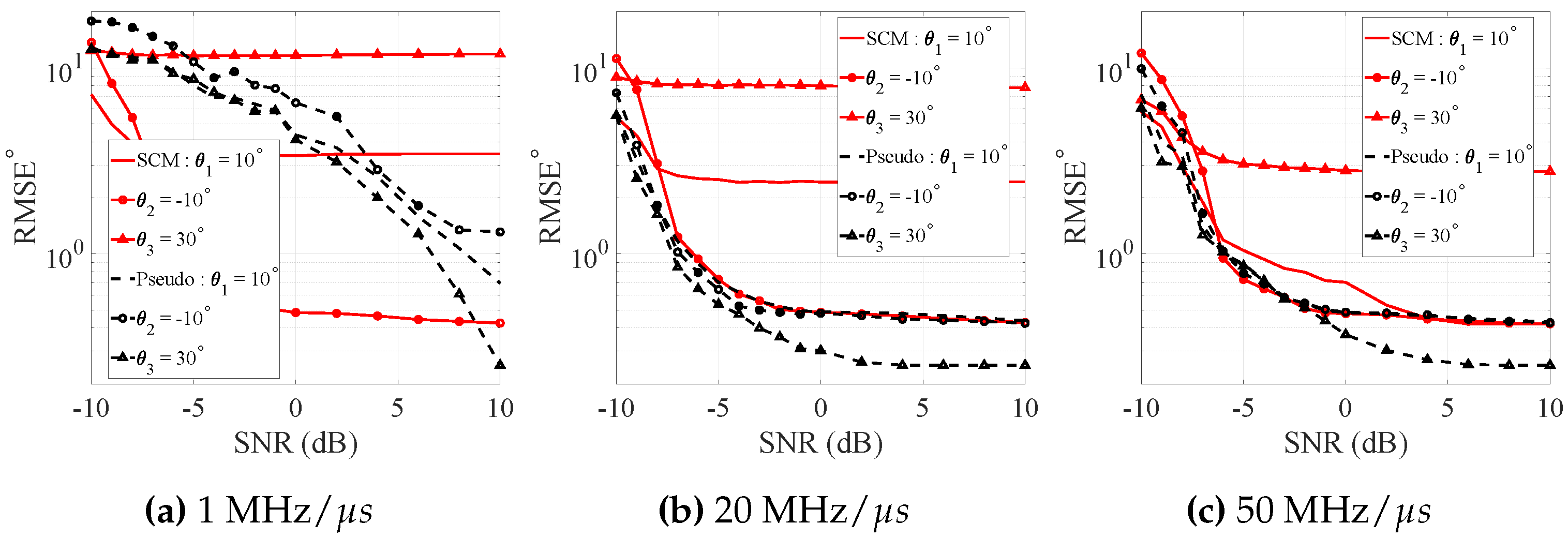
• The rmse is a statistical metric that quantifies the deviation of the estimates from the true DOA such that

  $$\begin{array}{c}\hfill RMS{E}_p\triangleq \sqrt{\frac{1}{R}\sum _{r=1}^R{\left({\widehat{\theta }}_{r,p}-{\theta }_{r,p}\right)}^2},\end{array}$$

  (11)

  where ${\widehat{\theta }}_{r,p}$ is the DOA estimate corresponding to a true DOA of ${\theta }_{r,p}$ of the pth signal in the rth iteration.

The next two subsections analyse the simulation results to investigate how different parameters affect the DOA estimation performance of single and multiple LFM signals. In the following sections, we analyse and discuss the results for the following cases. In Section 4.2.1, using plots of pseudospectra against DOA, we investigate the effect of the location of the initial frequency within the operational bandwidth on the DOA estimation performance. This investigation is done for a single emitter in both the narrowband and wideband cases for carrier frequencies of $8.0\mathrm{GHz}$ and $1.0\mathrm{GHz}$. Then, in Section 4.2.2, we analyse and discuss the results using the root mean-squared error (RMSE) of the DOA estimates. Section 4.3 and Section 4.4 extend the analysis to two and three emitters respectively, while also investigating the effects of symmetry.

4.2. DOA Estimation Performance for a Single Source

In this section, we investigate the DOA estimation performance for one LFM emitter situated at ${10}^{\circ }$ with negative chirp rates of $1\mathrm{MHz}/\mathsf{\mu }$s, $20\mathrm{MHz}/\mathsf{\mu }$s, and $50\mathrm{MHz}/\mathsf{\mu }$s and carrier frequencies of $8.0\mathrm{GHz}$ and $1.0\mathrm{GHz}$. The signals considered have initial frequencies of $f_{\min }+B_s/2$, $f_c+B_s/2$, and $f_{\max }$, where $B_s$ is the signal bandwidth. Firstly, in Section 4.2.1, we investigate the effect of the initial frequency on the DOA estimation performance using plots of spatial pseudospectra against DOA at $10\mathrm{dB}$ signal-to-noise ratio (SNR). We then investigate the DOA estimation performance using plots of RMSE against SNR in Section 4.2.2.

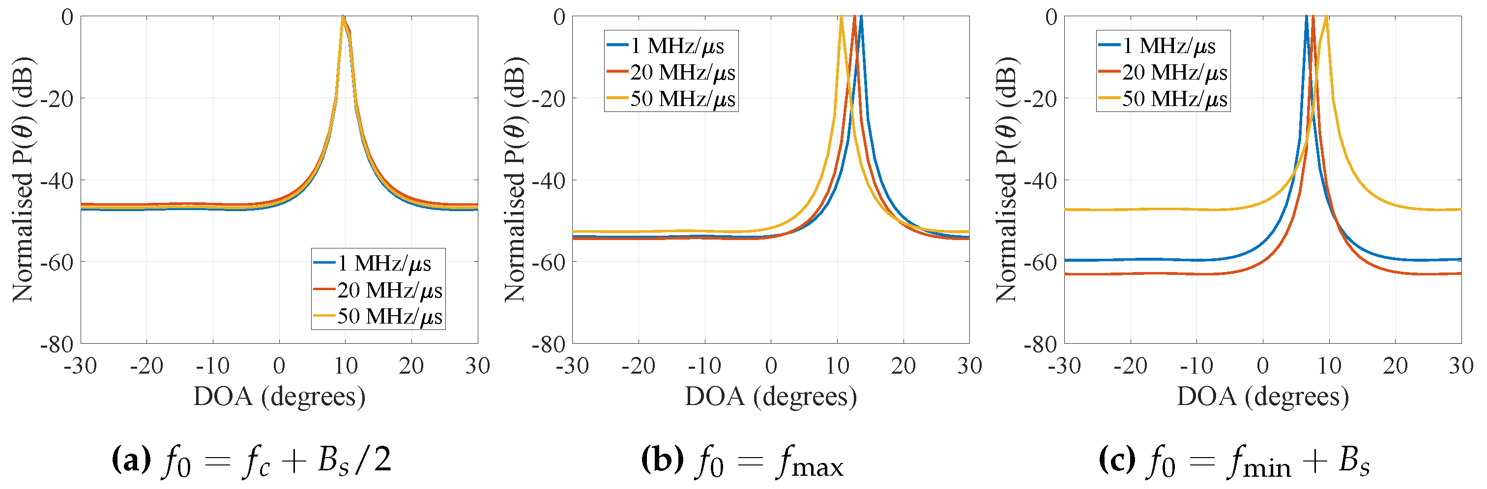
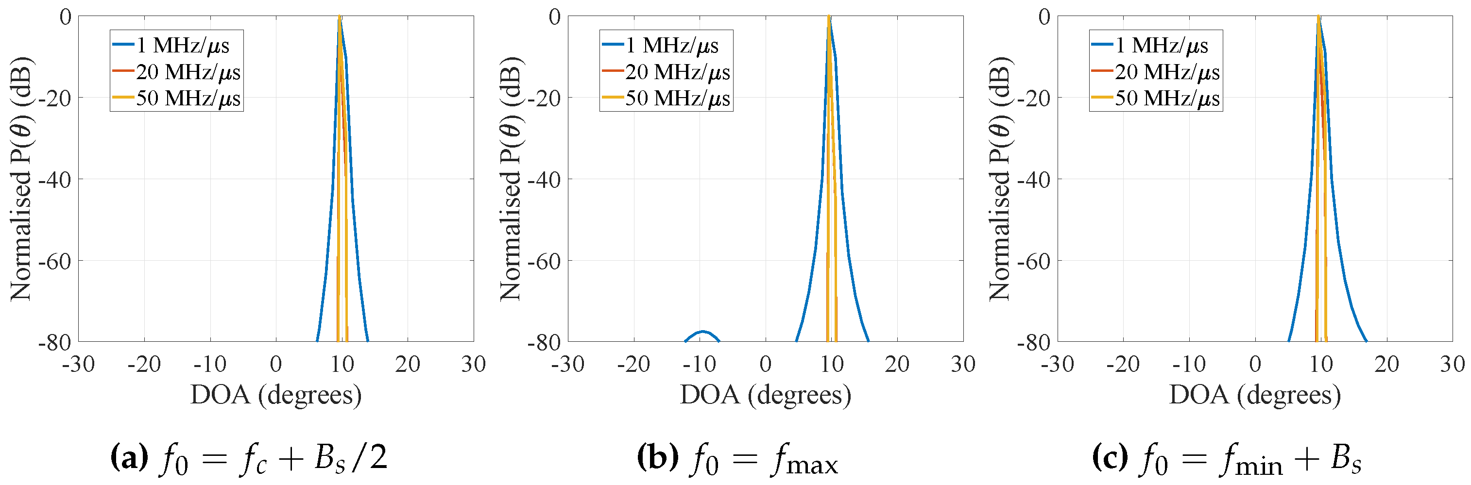
4.2.1. Effect of Initial Frequency

Figure 2, Figure 3, Figure 4 and Figure 5 show plots of the spatial pseudospectra for a single source against DOA for different initial frequencies of the LFM signal. Plots of pseudospectra for SCM-based aggregation with carrier frequencies of $8.0\mathrm{GHz}$ and $1.0\mathrm{GHz}$ are shown in Figure 2 and Figure 3, respectively. With SCM-based aggregation, the sharpest peak, which indicates the best DOA estimation can be observed with initial frequency of $f_c+B_s/2$, the case when the signal is closest and symmetric with respect to the carrier frequency. With the $8.0\mathrm{GHz}$ carrier frequency (Figure 2), the DOA estimates are visibly good as this is a narrowband case. For initial frequencies further away from the carrier frequency, that is, initial frequencies of $f_{\max }$ and $f_{\min }+B_s$, the DOA estimates are slightly worse than those obtained when the initial frequency is $f_c+B_s/2$. The DOA estimates for the initial frequencies that are away from the carrier frequency are only slightly worse because this is a narrowband case (Figure 2). With the $1.0\mathrm{GHz}$ carrier frequency (Figure 3), exact DOA estimates are only returned when the initial frequency coincides with the carrier frequency. Visibly large deviations of the DOA estimate from the true DOA occur when the initial frequencies of the chirp signals are further away from the carrier frequency (Figure 3). The deviations of the DOA estimate from the true DOA increase as the signal bandwidth increases. These large deviations are because the bandwidth of the signal is large relative to the carrier frequency (see Table 2). Plots of spatial pseudospectra against DOA for the pseudospectra-based aggregation with carrier frequencies of $8.0\mathrm{GHz}$ and $1.0\mathrm{GHz}$ are shown in Figure 4 and Figure 5, respectively. While some broadening of the peaks is visible with a carrier frequency of $8.0\mathrm{GHz}$, pseudospectra-based aggregation generally shows little variation in DOA estimation performance for all chirp rates.

4.2.2. Root-Mean-Squared Error (RMSE)

Figure 6 and Figure 7 show the variation of RMSE with SNR at carrier frequencies of $8.0\mathrm{GHz}$ and $1.0\mathrm{GHz}$, respectively. The DOA estimation performance for SCM-based aggregation is compared with that for the spatial pseudospectra aggregation technique with initial frequency $f_{\max }$. Performance results for LFM signals with carrier frequency of $8.0\mathrm{GHz}$ representing the narrowband case are shown in Figure 6. For the $1\mathrm{MHz}/\mathsf{\mu }$s chirp rate, spatial pseudospectra-based aggregation shows better estimation performance (lower RMSE values) compared to the SCM-based aggregation. The performance for the SCM-based aggregation and spatial pseudospectra aggregation converges at high SNR values. For the $20\mathrm{MHz}/\mathsf{\mu }$s and $50\mathrm{MHz}/\mathsf{\mu }$s chirp rates, both techniques show similar estimation performance trends. As the chirp rate increases, the estimation performance for SCM-based aggregation shows negligible variation at low SNR values and deteriorates slightly at high SNR. As the chirp rate increases, the estimation performance for spatial pseudospectra-based aggregation deteriorates slightly at low SNR but shows negligible variation at high SNR.

Performance results for LFM signals with the $1.0\mathrm{GHz}$ carrier frequency, representing the broadband case, are shown in Figure 7. For the $1\mathrm{MHz}/\mathsf{\mu }$s chirp rate, the RMSE for SCM-based estimation is poor and flat at about $3.5^{\circ }$ for SNR values higher than $-8\mathrm{dB}$. Spatial pseudospectra show significantly better estimation performance (with over $3^{\circ }$ lower RMSE) compared the performance for the SCM-based aggregation technique. For the $20\mathrm{MHz}/\mathsf{\mu }$s chirp rate, SCM-based aggregation shows some improvement (about $1^{\circ }$ for SNR values of at least $-8\mathrm{dB}$) compared to the case with $1\mathrm{MHz}/\mathsf{\mu }$s chirp rate. The RMSE curve flattens at about $1.5^{\circ }$ for SNR values beyond $-8\mathrm{dB}$. This performance is still significantly worse compared to that for spatial pseudospectra-based aggregation.

When the chirp rate increases to $50\mathrm{MHz}/\mathsf{\mu }$s, the performance for SCM-based aggregation improves significantly. In fact, both techniques show similar estimation performance for all SNR values. For all chirp-rates considered, the estimation performance for SCM-based aggregation deteriorates when the carrier frequency reduces from $8.0\mathrm{GHz}$ to $1.0\mathrm{GHz}$. The $50\mathrm{MHz}/\mathsf{\mu }$s chirp-rate signal shows the least performance deterioration as the carrier frequency reduces from $8.0\mathrm{GHz}$ to $1.0\mathrm{GHz}$. For all chirp rates, the estimation performance for spatial pseudospectra-based aggregation shows similar performance trends for carrier frequencies of $8.0\mathrm{GHz}$ and $1.0\mathrm{GHz}$. The estimation performance for spatial pseudospectra-based aggregation shows negligible variation as the carrier frequency decreases from $8.0\mathrm{GHz}$ to $1.0\mathrm{GHz}$, whereas with SCM-based aggregation, reducing the carrier leads to performance deterioration because the signals are narrowband with $8.0\mathrm{GHz}$ carrier frequency and wideband with $1.0\mathrm{GHz}$.

At the $8.0\mathrm{GHz}$ carrier frequency, the fractional bandwidths are small (Table 2). The LFM signals at each frequency bin are relatively close to the carrier frequency. In other words, the steering vectors associated with the bins containing the LFM signals of interest are very similar to the steering vector calculated at the carrier frequency. It must be noted that in the incoherent SCM-based aggregation method, after all the SCMs are combined, the pseudo spectrum is calculated using a single steering vector corresponding to the centre frequency. The slight performance deterioration as the chirp rate increases observed in Figure 2b can be attributed to the incoherence caused by the gradual deviation from the single steering vector assumption as the signal spreads over a wider bandwidth as discussed in Section 4.2.1. On the other hand, at the $1.0\mathrm{GHz}$ carrier frequency, the fractional bandwidths are much larger (Table 2).

The LFM signals are therefore non-coherent with respect to the carrier frequency. For low chirp rates, the frequency deviations of the frequency bins that contain signals are large and lead to large phase deviations from the steering vector, which is calculated at the centre frequency. These large phase deviations lead to performance degradation. This is exacerbated by addition of noise in the aggregation of SCMs from bins that do not contain a signal component. For signals with high chirp rates, the number of bins that contain the LFM signal increases. The spread of the phase deviations caused by the frequency bins that are not well-aligned to the carrier frequency average around zero and lead to improved DOA estimation performance (see Figure 3b). In spatial pseudospectra-based aggregation, the individual pseudospectra are calculated using the SCM and steering vector calculated for the corresponding frequency bin. Thus, the effect of coherence is not as severe because aggregation is performed in the spatial domain (Figure 4b and Figure 5b). As the number of bins containing the signal increases, the DOA estimation improves. This is because the steering vectors for more frequency bins that contain the signal combine coherently, leading to improved estimation performance.

4.3. DOA Estimation Performance for Two Sources

In this section, we investigate the DOA estimation performance of two LFM emitters that are situated symmetrically and non-symmetrically with respect to boresight. First, in Section 4.3.1, we consider two emitters situated symmetrically at ${10}^{\circ }$ and $-{10}^{\circ }$ with negative and positive chirp rates and with initial frequencies of $f_{\max }$ and $f_c-B_s/2$, respectively, where $B_s$ is the signal bandwidth. Signals with chirp rates of $1\mathrm{MHz}/\mathsf{\mu }$s, $20\mathrm{MHz}/\mathsf{\mu }$s, and $50\mathrm{MHz}/\mathsf{\mu }$s have been considered with carrier frequencies of $8.0\mathrm{GHz}$ and $1.0\mathrm{GHz}$. The non-symmetric case with emitters at ${10}^{\circ }$ and ${30}^{\circ }$ is discussed in Section 4.3.2. For both symmetric and non-symmetric cases, the DOA estimation performance has been investigated using plots of RMSE against SNR. Spatial pseudospectra have also been plotted for signals at carrier frequencies of $8.0\mathrm{GHz}$ and $1.0\mathrm{GHz}$ to demonstrate the effect of various parameters on the DOA estimation performance at $10\mathrm{dB}$ SNR.

4.3.1. Symmetrical sources situated at 10 and $-10$ degrees

Figure 8 and Figure 9 show plots of the RMSE against SNR for the two emitters, using both SCM-based and spatial pseudospectra-based aggregation, for the $8.0\mathrm{GHz}$ and $1.0\mathrm{GHz}$ carrier frequencies, respectively. With SCM-based aggregation at $8.0\mathrm{GHz}$, the DOA estimation performance for both emitters shows negligible variation as the chirp rate increases. For pseudospectra-based aggregation, the DOA estimation performance for both emitters improves as the chirp rate increases from $1\mathrm{MHz}/\mathsf{\mu }$s to $20\mathrm{MHz}/\mathsf{\mu }$s. However, the performance for both emitters deteriorates as the chirp rate increases from $20\mathrm{MHz}/\mathsf{\mu }$s to $50\mathrm{MHz}/\mathsf{\mu }$s. Both emitters show similar DOA estimation performance with SCM- and pseudospectra-based aggregation (see Figure 8). Performance variation for the $1.0\mathrm{GHz}$ carrier frequency is shown in Figure 9. For SCM-based aggregation, the DOA estimation performance for the emitter at ${10}^{\circ }$ improves as the chirp rate increases. This trend is similar to that observed for a single emitter (see Figure 7). However, the DOA estimation performance for the emitter at $-{10}^{\circ }$ deteriorates slightly as the chirp rate increases.

The performance for the emitter at $-{10}^{\circ }$ is significantly better compared to that for the emitter at ${10}^{\circ }$ for all chirp rates. The first emitter at ${10}^{\circ }$ with initial frequency of $f_{\max }$ is far away from the carrier frequency and shows performance similar to that observed in Figure 6 and Figure 7. The second emitter at $-{10}^{\circ }$ with initial frequency of $f_c-B_s/2$ is centred around the carrier frequency and results in better estimation performance because the steering vector for SCM-based aggregation coincides with the carrier frequency, as explained in Section 4.2.1. With pseudospectra-based aggregation, the DOA estimation performance for both emitters is similar and improves as the chirp rate increases from $1\mathrm{MHz}/\mathsf{\mu }$s to $20\mathrm{MHz}/\mathsf{\mu }$s for SNR values above $0\mathrm{dB}$. However, this DOA estimation performance shows negligible variation as the chirp rate increases from $20\mathrm{MHz}/\mathsf{\mu }$s to $50\mathrm{MHz}/\mathsf{\mu }$s. The DOA estimation performance for pseudospectra-based aggregation improves as the carrier frequency changes from $8.0\mathrm{GHz}$ to $1.0\mathrm{GHz}$.

Figure 10 and Figure 11 show plots of the spatial pseudospectra against DOA for emitters that are situated at ${10}^{\circ }$ and $-{10}^{\circ }$ for SCM-based and pseudospectra-based aggregation, respectively. Results for both $8.0\mathrm{GHz}$ and $1.0\mathrm{GHz}$ carrier frequencies are shown in each of these figures. For SCM-based aggregation, the peaks corresponding to the two emitters are clearly distinguishable at $8.0\mathrm{GHz}$ for all chirp rates considered. At $1.0\mathrm{GHz}$, however, only the $50\mathrm{MHz}/\mathsf{\mu }$s signal shows peaks located at the true DOA values. The peaks for the $1\mathrm{MHz}/\mathsf{\mu }$s and $20\mathrm{MHz}/\mathsf{\mu }$s signals show significant deviations from the true DOA values.

There is little variation in the pseudospectra at both carrier frequencies. For pseudospectra-based aggregation, the peaks corresponding to the two emitters coincide with the true DOA values of the emitters at both $8.0\mathrm{GHz}$ and $1.0\mathrm{GHz}$ carrier frequencies for all chirp rates considered. The peaks at the $1.0\mathrm{GHz}$ carrier frequency are much sharper compared to those at $8.0\mathrm{GHz}$. With both carrier frequencies, the $1\mathrm{MHz}/\mathsf{\mu }$s signal has broader peaks, which reveals worse DOA estimation performance compared to signals with the higher chirp rates of $20\mathrm{MHz}/\mathsf{\mu }$s and $50\mathrm{MHz}/\mathsf{\mu }$s due to the effect of the noise from the large number of frequency bins with no signal component. The peaks for pseudospectra-based aggregation at $10\mathrm{dB}$ SNR are sharper compared to peaks for SCM-based aggregation for both carrier frequencies, which implies that the spatial resolution for pseudospectra-based aggregation is better compared to that for SCM-based aggregation, at $10\mathrm{dB}$ SNR for all chirp rates considered.

4.3.2. Non-Symmetrical Sources

Using two emitters situated at ${10}^{\circ }$ and ${30}^{\circ }$, we investigate the effect of spatial symmetry on the DOA estimation performance for LFM signals with chirp rates of $1\mathrm{MHz}/\mathsf{\mu }$s, $20\mathrm{MHz}/\mathsf{\mu }$s, and $50\mathrm{MHz}/\mathsf{\mu }$s. Figure 12 and Figure 13 show plots of the RMSE against SNR, using both SCM-based and spatial pseudospectra-based aggregation, for $8.0\mathrm{GHz}$ and $1.0\mathrm{GHz}$ carrier frequencies, respectively. With SCM-based aggregation at $8.0\mathrm{GHz}$, the DOA estimation performance for both emitters shows negligible variation as the chirp rate increases. For SNR values less than $-3\mathrm{dB}$, the emitter at ${30}^{\circ }$ shows better DOA estimation performance compared to the emitter at ${10}^{\circ }$ for all chirp rates. However, for SNR values higher than $-3\mathrm{dB}$, the emitter at ${10}^{\circ }$ shows better DOA estimation performance compared to the emitter at ${30}^{\circ }$ for all chirp rates. For pseudospectra-based aggregation, the DOA estimation performance for both emitters improves as the chirp rate increases from $1\mathrm{MHz}/\mathsf{\mu }$s to $20\mathrm{MHz}/\mathsf{\mu }$s. However, the performance for both emitters deteriorates as the chirp rate increases from $20\mathrm{MHz}/\mathsf{\mu }$s to $50\mathrm{MHz}/\mathsf{\mu }$s. For all chirp rates and SNR values considered, the performance of the emitter at ${10}^{\circ }$ is worse than that of the emitter at ${30}^{\circ }$ (see Figure 12).

Performance variation for the $1.0\mathrm{GHz}$ carrier frequency is shown in Figure 13. For SCM-based aggregation, the DOA estimation performance for the emitter at ${10}^{\circ }$ improves as the chirp rate increases. This trend is similar to that observed for a single emitter (see Figure 7). However, the DOA estimation performance for the emitter at ${30}^{\circ }$ deteriorates slightly as the chirp rate increases. The performance for the emitter at ${30}^{\circ }$ is significantly better compared to that for the emitter at ${10}^{\circ }$ for both $1\mathrm{MHz}/\mathsf{\mu }$s and $20\mathrm{MHz}/\mathsf{\mu }$s chirp rates. With the $50\mathrm{MHz}/\mathsf{\mu }$s chirp rate, however, the DOA estimation performance of the two emitters is comparable. With pseudospectra-based aggregation, the DOA estimation performance for both emitters improves as the chirp rate increases from $1\mathrm{MHz}/\mathsf{\mu }$s to $20\mathrm{MHz}/\mathsf{\mu }$s but shows negligible variation as the chirp rate increases from $20\mathrm{MHz}/\mathsf{\mu }$s to $50\mathrm{MHz}/\mathsf{\mu }$s. For all chirp rates and SNR values considered, the emitter at ${10}^{\circ }$ shows slightly better estimation performance compared to the emitter at ${30}^{\circ }$. While the performance trends of the emitter at ${10}^{\circ }$, using SCM-based aggregation, are similar for both $8.0\mathrm{GHz}$ and $1.0\mathrm{GHz}$ carrier frequencies, there is noticeable performance degradation with pseudospectra-based aggregation especially at the $8.0\mathrm{GHz}$ carrier frequency.

Figure 14 and Figure 15 show plots of the spatial pseudospectra against DOA for SCM-based and pseudospectra-based aggregation respectively. Results for both $8.0\mathrm{GHz}$ and $1.0\mathrm{GHz}$ carrier frequencies are shown in each of these figures. These plots are generated for emitters situated at ${10}^{\circ }$ and ${30}^{\circ }$ for $10\mathrm{dB}$ SNR. For SCM-based aggregation, the peaks corresponding to the two emitters coincide with the true DOA values, for all chirp rates considered at the $8.0\mathrm{GHz}$ carrier frequency. At the $1.0\mathrm{GHz}$ carrier frequency, however, only the $50\mathrm{MHz}/\mathsf{\mu }$s chirp rate shows peaks located close to the true DOA values. The peaks for the $1\mathrm{MHz}/\mathsf{\mu }$s and $20\mathrm{MHz}/\mathsf{\mu }$s chirp rates are significantly far away from the true DOA values (Figure 14). The peaks for pseudospectra-based aggregation are sharper than the peaks for SCM-based aggregation for both $8.0\mathrm{GHz}$ and $1.0\mathrm{GHz}$ carrier frequencies with all chirp rates (Figure 15). This implies that pseudospectra-based aggregation has better spatial resolution compared to SCM-based aggregation for all chirp rates considered.

4.4. DOA Estimation Performance for Three Sources

Using three emitters situated at ${10}^{\circ }$, $-{10}^{\circ }$, and ${30}^{\circ }$, we investigated the DOA estimation performance for LFM signals with chirp rates of $1\mathrm{MHz}/\mathsf{\mu }$s, $20\mathrm{MHz}/\mathsf{\mu }$s, and $50\mathrm{MHz}/\mathsf{\mu }$s. The three emitters have initial frequencies of $f_{\max }$, $f_c-B_s/2$, and $f_{\min }$, respectively. Figure 16 and Figure 17 show plots of the RMSE against SNR, using both SCM-based and spatial pseudospectra-based aggregation, for $8.0\mathrm{GHz}$ and $1.0\mathrm{GHz}$ carrier frequencies, respectively. With SCM-based aggregation at $8.0\mathrm{GHz}$, the estimation performance for all chirp rates considered is similar because this is a narrowband case (Figure 16). In the wideband case at $1.0\mathrm{GHz}$, with SCM-based aggregation, the emitter at $-{10}^{\circ }$ shows better estimation performance than the emitters at ${10}^{\circ }$ and ${30}^{\circ }$ for all chirp rates considered (Figure 17). This is because the signal at $-{10}^{\circ }$ is centred around the carrier frequency whereas the emitters at ${10}^{\circ }$ and ${30}^{\circ }$ are further away. The performance trends observed in Figure 16 and Figure 17 for three emitters are similar to those depicted in Figure 6 and Figure 7 for a single emitter and in Figure 8, Figure 9, Figure 10, Figure 11, Figure 12 and Figure 13 for two emitters.

The spatial pseudospectra for the three emitters against DOA for SCM-based and pseudospectra-based aggregation are shown in Figure 18 and Figure 19, respectively. Results at $10\mathrm{dB}$ SNR for both $8.0\mathrm{GHz}$ and $1.0\mathrm{GHz}$ carrier frequencies are shown in each of these figures. With SCM-based aggregation, the peaks for each of the three emitters coincide with the true DOA in the narrowband case at $8.0\mathrm{GHz}$. However, in the wideband case at $1.0\mathrm{GHz}$, only peaks for the emitter at $-{10}^{\circ }$ coincide with the true DOA, because the emitter at $-{10}^{\circ }$ is centred around the carrier frequency (Figure 18). With pseudospectra-based aggregation, all three emitters are clearly distinguishable in both narrowband and wideband cases (Figure 19).

4.5. Summary of DOA Estimation Performance Results

Under some circumstances such as low fractional bandwidth and/or large signal of interest occupancy in a given analysis bandwidth, SCM-based aggregation can achieve good estimation performance while offering lower computational complexity as this technique does not need to compute a spatial pseudospectrum for every frequency bin. This simpler technique, however, does not yield good estimation results for signals that are wideband and not closely aligned to the carrier frequency. The pseudo spectra-based aggregation technique gives better performance for the wideband emitter scenario due to the aggregation in the spatial domain. The above findings are consistent for both single and multiple emitters.

4.6. Computational Complexity Analysis

This section highlights the computational costs involved in the implementation of the considered aggregation techniques for the different parameters involved. The results for simulation time presented in this section were obtained from simulations in MATLAB by performing computations sequentially using a central processing unit (CPU)-based platform (Processor: Intel(R) Core (TM) $i7-6700T$ CPU with $2.80\mathrm{GHz}$ and $2.81\mathrm{GHz}$, and $16.0\mathrm{GB}$ memory (RAM), running Windows 10 Enterprise).

The computational cost of the MUSIC algorithm, its variants, and the steps involved have been studied in [16,26,27].

Table 3. Computational complexity for the major processing steps in SCM-based and pseudospectra-based aggregation with narrowband MUSIC.

Complexity (Flops)	SCM-Based	Psuedospectra-Based
for $100\mathsf{\mu }$s	Aggregation	Aggregation
Computation of scms	$\lfloor J/K\rfloor \times \mathcal{O}\left(M^2\right)$	$\lfloor J/K\rfloor \times \mathcal{O}\left(M^2\right)$
Computation of evd	$N_Q\times \mathcal{O}\left(M^2(P+2)\right)$	$N_{Q}K\times \mathcal{O}\left(M^2(P+2)\right)$
Spectral search	$N_{\theta }\times \mathcal{O}\left((M+1)(M-P)\right)$	$N_{\theta }\times \mathcal{O}\left((M+1)(M-P)\right)$
Simulation time (ms)	$17.8$	$145.5$

shows the computational complexity (in flops) of the predominant steps involved in the spatial pseudospectra-based aggregation. SCM-based aggregation requires the eigenvalue decomposition (EVD) step once and the peak searching step once for every time block. Pseudospectra-based aggregation on the other hand requires the EVD step K times and the peak searching step once. With the 100 bins considered in these simulations, pseudospectra-based aggregation requires 100 times more EVD computations compared to SCM-based aggregation. Table 3 also shows the average simulation time required for both SCM-based aggregation and spatial pseudospecta-based aggregation. Spatial pseudospectra-based aggregation requires about 8 times more simulation time (∼146 $\mathrm{ms}$) compared to that required by SCM-based aggregation (∼18 $\mathrm{ms}$) for the parameters considered using the same computing platform. Note that if a parallel high-speed computing architecture is available then the K EVD calculations required by the pseudospectra method can be parallelised as these calculations are independent of each other. The computational complexity associated with incoherent DOA estimation techniques is significantly lower than the computational complexity associated with coherent DOA estimation techniques. This is because, in addition to the eigendecomposition step, coherent techniques such as CSSM and TOPS also require matrix inversion [28].

5. Conclusions

This article has evaluated the DOA estimation performance for both narrowband and wideband LFM signals using spatial covariance matrix (SCM)-based and pseudospectra-based incoherent aggregation techniques. We have analysed the effect of fractional bandwidth and that of the fraction of frequency bins containing the desired signals on the performance of these techniques. We have also identified scenarios in which the lower-complexity SCM-based aggregation technique (about 10 times less complexity) can yield relatively good DOA estimation performance compared to pseudospectra-based aggregation. SCM-based aggregation is appealing for cases in which the frequency bins containing the signal are closely aligned to the centre frequency. Relatively good estimation performance can be achieved in such scenarios, for both single and multiple emitters, with much lower computational complexity compared to the spatial pseudospectra-based aggregation technique. The latter offers good DOA estimation performance for low-power, wideband single emitters. Future research will consider possible improvements of estimation performance and further reduction of complexity for both incoherent SCM-based aggregation and incoherent spatial pseudospectra-based aggregation.

References

1. Tsui, J.; Cheng, C.H. Digital Techniques for Wideband Receivers, 3rd ed.; Institution of Engineering and Technology: London, UK, 2016. [Google Scholar]
2. Krim, H.; Viberg, M. Two decades of array signal processing research: The parametric approach. IEEE Signal Process. Mag. 1996, 13, 67–94. [Google Scholar] [CrossRef]
3. Schmidt, R. Multiple emitter location and signal parameter estimation. IEEE Trans. Antennas Propag. 1986, 34, 276–280. [Google Scholar] [CrossRef] [Green Version]
4. Roy, R.; Kailath, T. ESPRIT-Estimation of signal parameters via rotational invariance techniques. IEEE Trans. Acoust. Speech Signal Process. 1989, 37, 984–995. [Google Scholar] [CrossRef] [Green Version]
5. Akaike, H. A new look at the statistical model identification. IEEE Trans. Autom. Control. 1974, AC-19, 716–723. [Google Scholar] [CrossRef]
6. Wax, M.; Kailath, T. Detection of signals by information theoretic criteria. IEEE Trans. Acoust. Speech Signal Process. 1988, ASSP-33, 387–392. [Google Scholar] [CrossRef] [Green Version]
7. Su, G.; Morf, M. The signal subsapace approach for multiple wide-band emitter location. IEEE Trans. Acoust. Speech Signal Process. 1983, ASSP-31, 1502–1522. [Google Scholar]
8. Yoon, Y.S.; Kaplan, L.M.; McClellan, J.H. TOPS: New DOA estimator for wideband signals. IEEE Trans. Signal Process. 2006, 54, 1977–1989. [Google Scholar] [CrossRef]
9. Yu, H.; Liu, J.; Huang, Z.; Zhou, Y.; Xu, X. A new method for wideband DOA estimation. In Proceedings of the 2007 International Conference on Wireless Communications, Networking and Mobile Computing, WiCOM 2007, Shanghai, China, 21–25 September 2007; pp. 598–601. [Google Scholar] [CrossRef]
10. Wang, H. Coherent signal-subspace processing for the detection wide-band sources. IEEE Trans. Acoust. Speech Signal Process. 1985, ASSP-33, 823–831. [Google Scholar] [CrossRef] [Green Version]
11. Di Claudio, E.D.; Parisi, R. WAVES: Weighted average of signal subspaces for robust wideband direction finding. IEEE Trans. Signal Process. 2001, 49, 2179–2191. [Google Scholar] [CrossRef] [Green Version]
12. Okane, K.; Ohtsuki, T. Resolution improvement of wideband direction-of-arrival estimation “Squared-TOPS”. In Proceedings of the IEEE International Conference on Communications, Cape Town, South Africa, 23–27 May 2010; pp. 1–6. [Google Scholar] [CrossRef]
13. Zhang, L.; Liu, W.; Langley, R.J. A Class of constrained adaptive beamforming algorithms based on uniform linear arrays. IEEE Trans. Signal Process. 2010, 58, 3916–3922. [Google Scholar] [CrossRef]
14. Hayashi, H.; Ohtsuki, T. DOA estimation for wideband signals based on weighted Squared TOPS. Eurasip J. Wirel. Commun. Netw. 2016, 2016. [Google Scholar] [CrossRef] [Green Version]
15. Shaw, A.K. Improved Wideband DOA Estimation Using Modified TOPS (mTOPS) Algorithm. IEEE Signal Process. Lett. 2016, 23, 1697–1701. [Google Scholar] [CrossRef]
16. Selva, J. Efficient wideband DOA estimation through function evaluation techniques. IEEE Trans. Signal Process. 2018, 66, 3112–3123. [Google Scholar] [CrossRef] [Green Version]
17. Bai, Y.; Li, J.; Wu, Y.; Wang, Q.; Zhang, X. Weighted Incoherent Signal Subspace Method for DOA Estimation on Wideband Colored Signals. IEEE Access 2019, 7, 1224–1233. [Google Scholar] [CrossRef]
18. Pace, P.E. Detecting and Classifying Low Probability of Intercept Radar; Artech House: Norwood, MA, USA, 2008. [Google Scholar]
19. Amin, M.G.; Zhang, Y.D. DOA estimation of nonstationary signals. In Academic Press Library in Signal Processing: Volume 3 Array and Statistical Signal Processing; Elsevier Ltd.: Amsterdam, The Netherlands, 2014; Volume 3, pp. 765–798. [Google Scholar] [CrossRef]
20. Mulinde, R.; Dissanayake, D.W.; Kaushik, M.; Ho, S.W.; Chan, T.; Attygalle, S.M.; Aziz, S.M. DOA estimation of wideband LFM RARAR Signals. In Proceedings of the International Radar Conference, Toulon, France, 23–27 September 2019; pp. 1–6. [Google Scholar] [CrossRef]
21. Mulinde, R.; Kaushik, M.; Attygalle, M.; Aziz, S.M. Evaluation of aggregation techniques for DOA estimation of wideband radar signals. In Proceedings of the 2020 14th International Conference on Signal Processing and Communication Systems, ICSPCS 2020, Adelaide, SA, Australia, 14–16 December 2020; pp. 1–9. [Google Scholar] [CrossRef]
22. Amin, M.G.; Zhang, Y. Direction finding based on spatial time-frequency distribution matrices. Digit. Signal Process. A Rev. J. 2000, 10, 325–359. [Google Scholar] [CrossRef] [Green Version]
23. Mulinde, R.; Attygalle, M.; Aziz, S.M. Experimental validation of direction of arrival estimation for high chirp-rate linear frequency modulated radar signals. IET Radar Sonar Navig. 2021, 15, 627–640. [Google Scholar] [CrossRef]
24. Guo, R.; Zhang, Y.; Lin, Q.; Chen, Z. A channelization-based DOA estimation method for wideband signals. Sensors 2016, 16, 1031. [Google Scholar] [CrossRef] [Green Version]
25. Blunt, S.D.; Jakabosky, J.; Mccormick, P.; Tan, P.S.; Metcalf, J.G. Holistic radar waveform diversity. In Academic Press Library in Signal Processing Volume 7; Elsevier Ltd.: Amsterdam, The Netherlands, 2018; Volume 7, pp. 3–50. [Google Scholar] [CrossRef]
26. Yan, F.; Jin, M.; Qiao, X. Low-complexity DOA estimation based on compressed MUSIC and its performance analysis. IEEE Trans. Signal Process. 2013, 61, 1915–1930. [Google Scholar] [CrossRef]
27. Sun, F.; Lan, P.; Gao, B.; Chen, L. A low complexity direction of arrival estimation algorithm by reinvestigating the sparse structure of uniform linear arrays. Prog. Electromagn. Res. C 2016, 63, 119–129. [Google Scholar] [CrossRef] [Green Version]
28. Kulhandjian, H.; Kulhandjian, M.; Kim, Y.; D’Amours, C. 2-D DOA estimation of coherent wideband signals with auxiliary-vector basis. In Proceedings of the International Conference on Communications Workshops, Kansas City, MO, USA, 20–24 May 2018; pp. 1–6. [Google Scholar] [CrossRef]
Figure 1. Illustration of the two incoherent aggregation techniques. Reprinted with permission from ref. [21]. Copyright 2021 IEEE.
Electronics 10 01707 g001
Figure 2. Spatial pseudospectra for SCM-based aggregation with different initial frequencies for a signal at 10 and f c = 8.0 GHz .
Electronics 10 01707 g002
Figure 3. Spatial pseudospectra for SCM-based aggregation with different initial frequencies for a signal at 10 and f c = 1.0 GHz .
Electronics 10 01707 g003
Figure 4. Spatial pseudospectra for pseudospectra-based aggregation with different initial frequencies for a signal at 10 and f c = 8.0 GHz .
Electronics 10 01707 g004
Figure 5. Spatial pseudospectra for pseudospectra-based aggregation with different initial frequencies for a signal at 10 and f c = 1.0 GHz .
Electronics 10 01707 g005
Figure 6. Variation of RMSE with SNR at f c = 8.0 GHz for different chirp rates for a signal at 10 with initial frequency f max .
Electronics 10 01707 g006
Figure 7. Variation of RMSE with SNR at f c = 1.0 GHz for different chirp rates for a signal at 10 with initial frequency f max .
Electronics 10 01707 g007
Figure 8. Variation in RMSE with SNR with different chirp rates for two signals at 10 and 10 , f c = 8.0 GHz , with initial frequencies f max and f c B s / 2 .
Electronics 10 01707 g008
Figure 9. Variation in RMSE with SNR with different chirp rates for two signals at 10 and 10 , f c = 1.0 GHz , with initial frequencies f max and f c B s / 2 .
Electronics 10 01707 g009
Figure 10. Spatial pseudospectra for SCM-based aggregation for two signals at 10 and 30 , with SNR = 10 dB , for different chirp rates.
Electronics 10 01707 g010
Figure 11. Spatial pseudospectra for pseudospectra-based aggregation for two signals at 10 and 30 , with SNR = 10 dB , for different chirp rates.
Electronics 10 01707 g011
Figure 12. Variation in RMSE with SNR with different chirp rates for two signals at 10 , 30 degrees, f c = 8.0 GHz , with initial frequencies f max and f c B s / 2 .
Electronics 10 01707 g012
Figure 13. Variation in RMSE with SNR with different chirp rates for two signals at 10 , 30 degrees, f c = 1.0 GHz , with initial frequencies f max and f c B s / 2 .
Electronics 10 01707 g013
Figure 14. Spatial pseudospectra for SCM-based aggregation for two signals at 10 and 30 , with SNR = 10 dB , for different chirp rates.
Electronics 10 01707 g014
Figure 15. Spatial pseudospectra for pseudospectra-based aggregation for two signals at 10 and 30 , with SNR = 10 dB , for different chirp rates.
Electronics 10 01707 g015
Figure 16. Variation in RMSE with SNR at f c = 8.0 GHz for different chirp rates for three signals at 10 , 10 , and 30 , with initial frequencies f max , f c B s / 2 , and f min .
Electronics 10 01707 g016
Figure 17. Variation in RMSE with SNR at f c = 1.0 GHz for different chirp rates for three signals at 10 , 10 , and 30 , with initial frequencies f max , f c B s / 2 , and f min .
Electronics 10 01707 g017
Figure 18. Spatial pseudospectra for SCM-based aggregation for three signals at 10 , 10 , and 30 , with SNR = 10 dB , for different chirp rates.
Electronics 10 01707 g018
Figure 19. Spatial pseudospectra for pseudospectra-based aggregation for three signals at 10 , 10 , and 30 , with SNR = 10 dB , for different chirp rates.
Electronics 10 01707 g019