Abstract
In 1983, B. Moszkowski introduced a first interval-interpreted temporal logic system, the so-called Interval Temporal Logic (ITL), as a system suitable to express mutual relations inside intervals for reasonings about digital circuits. In 1991, Halpern and Shoham proposed a new temporal system (HS) to describe external relations between intervals. This paper is aimed at proposing a basis-type combination of HS and a simplified ITL end extends it towards a multi-valued system—also capable of rendering a gradable justification of agents in a similar contexts of reasoning about digital circuits. This newly introduced system is semantically interpreted in the so-called fibred semantics.
1. Introduction
1.1. The Interval Temporal Logic Systems
The majority of realistic requirements-imposed on different IT-systems (they may refer to their liveness, safety, or activity.) often require temporal logic systems with non-pointwise semantics to be properly represented formally. Different context-oriented analysis and observations, f.e. from [1,2,3], visualized a need to explore interval-based semantics temporal logic systems in many engineering contexts, such as reasoning about digital circuits or specification of the instruction set processors.
The observations seemed to motivate B. Moszkowski to propose a complex frame of the interval-based temporal logic system—recognized as ‘Interval Temporal Logic’ (ITL) and introduced in [4,5]. Its utility manifests itself in its capability of uniformly describing the structure and dynamics of timing-dependent digital circuits. A potential application area of this formal system is determined by various devices, including the delay elements, adders, latches, counters, flip-flops, random-access memories, or a clocked multiplication circuit.
Whereas ITL forms a multi-modal system adaptable to represent temporal (internal) relations between intervals and their subintervals, such as next, begin, fin, halt, keep and yield, its younger sister to be called Halpern–Shoham logic (HS) constitutes a multi-modal logic suitable to represent the so-called Allen’s temporal relations between (mutually external) intervals (see: [6]). It was introduced and described in detail by Halpern and Shoham in [7]. This primary difference between these two formal systems finds its further extensions in mutually different directions of exploring these systems. In fact, whereas HS has been intensively explored in such works as [8,9,10,11]) mainly from a metalogical perspective, ITL is usually discussed in different contexts of programming-applicable specification for such formal features of IT systems (hardware, software, etc.) as liveness or safety. This fact finds its reflection in such works as: [5,12,13,14].
1.2. Verifiability and Provability Logic
Whereas different components of a purely temporal provenance (such as internal temporal relations inside a given interval or external temporal relations between intervals) may be expressed either by ITL or HS and semantically interpreted in their models, the situation makes more complicated if additionally consider some epistemic ‘entities’, such as beliefs or preferences. The same difficulty arises for other epistemic abstract properties, such as provability, verifiability (these properties as some attributes of other features or facts may be reformulated as properties of ‘being provable’ or ‘being verifiable’). Usually, the notion of provability has a purely formal pragmatic meaning and is exploited concerning formal theories, such as Peano Arithmetic, set theory, formal systems of temporal logic: LTL, CTL, etc. Due to Hempel’s and post-Hempel critique of neo-positivistic verificationism in contemporary philosophy of science and general methodology—the notion of confirmation instead of verification is more suitable to all theories interpreted empirically, such as theories of physics or theories in technical sciences. (see: [15]). Slightly against this tradition, we decide to explore the concept of ‘verification’. We make it not because of reverence to neo-positivistic verificationism, but because of some recapitulation of use of the concept in different application-based context by model checking and the so-called formal verification—due to [16,17,18].), observability as some attributes of facts, other properties or—directly—of objects, events, and relations between them. In particular, no formal representation of verifiability, i.e., a formal representation of ‘being verifiable’, has been elaborated. However, a formalization attempt for this concept may be supported by the formalization tradition suitable to the concept of provability. It stems from the ground-breaking K. Gödel’s incompleteness theorems for Peano Arithmetic (PA) from 1931 (see: [19]) and Löb’s modal-based formalization of the so-called Hilbert–Bernays provability conditions for PA from [20]. If is a provability predicate for formulae of PA ( stands for ‘A is provable in PA’) and PA⊢ denotes PA-derivability, then the Löb’s conditions may be depicted in the form of axioms:
- 1.
- If PA , then PA ,
- 2.
- PA ,
- 3.
- PA ,
where denotes the Gödel’s number of (PA).
These conditions may be naturally reformulated to a modal form and—as such ones—constitute the axioms of provability logic, often called: ‘Gödel–Löb logic’ and denoted by GL.
These conditions may be naturally reformulated to a modal form and—as such ones—constitute the axioms of provability logic, often called: ‘Gödel–Löb logic’ and denoted by GL.
1.3. Paper Motivation and Initial Problem Formulation
Unfortunately, not only the lack of the appropriate formalization pattern for the concept of verifiability constitutes a challenging difficulty. Indeed, formal languages of HS and ITL as taken separately—even built up from a description logic—are insufficient because of various conceptual limitations.
- •
- Both systems—ITL and HS—are only suitable to express internal and external temporal relations (resp.) and cannot grasp their combinations.
- •
- Existing types of semantics for these systems usually are not sensitive to different pragmatic aspects of the modeled situations that should be considered from the perspective of the requirement of their adequacy and realism.
- •
- Even if a piece of pragmatics is considered in these types of semantics—such as in the so-called Fagin’s behavioral one from [21]—they are not suitable to model the combined formulae for a temporal and a non-temporal type.
- •
- Even combined formal systems, such as epistemic HS from [22], describe some unrealistically idealized epistemic capabilities of agents.
- •
- Last, but not least—due to author’s best knowledge—no more advanced model checking machinery has been yet elaborated for digital circuit’s properties and behavior—against so sophisticated attempts to adopt bounded model checking for microprocessor architectures—as in [23].
In order to formulate the initial problem for its further representation in our multi-valued HS-based modeled extension of ITL and modeling in its models—one needs to underline the extraordinary suitability of ITL from [4] to grasp the digital circuit’s behavior and properties. Moszkowski’s formalization attempt refers to different types of computational circuits, such as adders (see: [4], pp. 55–64), multipliers (see: [4], pp. 86–88) or the data handling combinational circuits, such as Multiplexer (see: [4], pp. 86–88) and many others. It is noteworthy to see that the monadic predicate version of ITL is exploited to express such entities as bits or signals through some unique model operators (We omit a detailed explanation of their semantics.) as a formal representation of the phrases: ‘for all internal subintervals (of a given one),’ ‘for all terminal subintervals’ and ‘for all internal subintervals’ (resp.) For example, two predicates bit and Bit are used to represents bits: the predicate bit checks if a value is either 0 or 1 and the predicate Bit checks that its parameter is always bit-valued —due to the formal depiction in [4], p. 29:
Putting aside the whole taxonomy of ITL predicates, one can observe that some of them are especially useful and play the role of technical predicates to be exploited in further formalization attempts. One of them is the ‘LoadPhase’ predicate. Due to [4], p. 107—the predicate ’LoadPhase’ specifics device operation for initially loading the inputs.
Independently of these types of formalization attempts—often arises a need to formally specify and adequately model different integrated systems and complicated scenarios, such as the reasoning of an operating agent (with epistemic capabilities) about processes in the world of digital circuits. An exemplary situation of this type, for which formalization of the ’LoadPhase’ predicate is used, is described in the following Motivating Example.
The Motivating Example 1.
Let us consider an agent-observer i, which supervises some fragment of the ‘loading phase’ action performing and let us assume that it verifies with some degree α a (materialization of its) subprocess ‘after some time (later): initially was H and finally ‘status = 1’ occurred’.
In order to specify the situation described in the Motivating Example—it is convenient to start from the ITL-formula defining the process of loading phase as follows (This ITL-formula delivers a more general scheme of representing some types of actions (similar to ‘LoadPhase’ above) in terms of the appropriately specified atomic formulae (like ‘Load(H)’, ‘Init(H)’, ‘status=1’ above) using a modal-type operator (like: ‘fin’). The Formula (1) constitutes a convenient basis for further extensions and is sensitive to further modifications and combinations. These possibilities seem to justify a paradigmatic nature of the formula, although one could indicate other formulae for this analysis.) (see: [4], p. 108):
It easy to see that (1) may be reformulated to a new Formula (2) involved in a new HS-modal operator:
which renders the temporal action sequencing—previously rendered mainly by → in terms of HS-modal operator [L] (for ‘Later’) of the box-type. However—in order to adequately express the scenario from the Motivating Example—we need a new epistemic modal-type operator, say which expresses the agent i verification of (an event, a process, etc.) with a degree (This formula is read ‘An agent i verifies with a degree .’ Intentionally, we intend to consider a finite set of such possible degrees of agent verification of the given event or processes, etc. They might be dependent on their observability, but we put aside this type of considerations as redundant from the perspective of the paper analysis.).
This fact may be rendered by the following combined formula:
The example will constitute a practical component of the main objective of the paper analysis-to find the appropriate semantics suitable to model the formulae of the same sort.
Unfortunately, some further difficulties and limitations of this task should be taken into account. Fortunately, they simultaneously indicate the direction of the task materialization.
- The full ITL is too excessive for the requirements. Thus we restrict ITL to its propositional variant.
- Some fragments (f.e. these of the arithmetic nature) of the propositional ITL—as defined in [4]—seem to be already too heterogeneous to constitute a convenient starting point of the hybrid system construction. Therefore, these arithmetic-based fragments of ITL will be replaced by the corresponding description-logic formulae.
- Finally, Gödel–Löb logic of provability cannot be adapted as an adequate logic for gradable verifiability, but it partially delivers a pattern or a surrogate for it. Therefore, it will be exploited in a role of basis in the hybrid formal system construction process.
- Last, but not least—Gabbay’s frame of the so-called fibred semantics from [24] exists for a point-wise semantics only, but it seems to be adaptable to an interval-based semantics. Thus, it will be used in the paper.
1.4. Objectives of the Paper
Due to the motivation factors-the main objectives of the paper are (in chronological order):
- to propose a multi-valued logic for gradable verifiability (MVer),
- to introduce a new hybrid system MVHSM as a unique combination of Halpern–Shoham Logic, Simplified Interval Temporal Logic of Moszkowski and multi-valued logic for gradable verifiability (MVer) (a specification of the combination will be explained in details later.)
- to elaborate a general frame of the interval counterpart of Gabbay’s fibred semantics,
- to semantically interpret the newly introduced MVHS in the fibred interval semantics,
- to describe a general frame of model checking for MVHSM and its possible extensions.
From a more practical perspective, this paper is aimed at proposing a potentially paradigmatic method of semantic modeling of agent’s reasoning about digital circuits in terms of the combined MVHSM system.
One needs to underline that the paper belongs to the common intersection of research on temporal logic systems and knowledge representation as a part of AI. As such, the paper does not refer to digital circuits themselves in their electronics-based depiction (In fact, we rather consider them in a slightly more idealized perspective, i.e., as unique acyclic directed graphs.), but it refers to their formal properties and pieces of reasoning about them—as expressible in MVHSM and its potential extensions. One should underline that the deceptively purely logical nature of these analyses is essentially oriented for the idea of a combined model checking of both formal properties of digital circuits and pieces of reasoning about them.
Reasoning about them constituted the primary motivating factor for the construction of Moszkowski’s Interval Temporal Logic. Meanwhile, this system forms one of two pillars of the newly constructed MVHSM system.
1.5. Organization of Paper
The rest of the paper is organized as follows. In Section 2, a terminological framework of analysis is put forward. In Section 3, a simplified Halpern–Shoham- Moszkowski Logic (HSM) is introduced syntactically. A Multi-Valued Verifiability Logic (MVer) is presented in Section 4 syntactically and semantically. In Section 5, the hybrid system of Multi-Valued Simplified Halpern–Shoham–Moszkowski Logic for Gradable Verifiability (MVHSM) is introduced and semantically interpreted in the interval fibred semantics. Section 6 explains a broader model checking-orientation of the paper analysis. In Section 7, state of the art is described. Section 8 contains the final remarks and conclusions.
2. Terminological Framework
Before we move to the right part of the paper, a conceptual apparatus —for ITL and HS and their semantic interpretations in the Kripke frame-based models will be put forward. We start its presentation from the so-called Interval-Based Interpreted System (IBIS) as unique transition systems. Although we intend to exploit Kripke frame-based models as a basis for the so-called fibred semantics for the hybrid MVHSM system, it seems reasonable to begin with transition systems. This solution gives an excellent opportunity to grasp deep relationships between them and their corresponding Kripke frames and an internal organization of Kripke frames. Finally, it enables understanding how discrete intervals may be created.
Secondly, a simplified ITL and Halpern-Shoam logic are presented in their syntactic and semantic depictions.
2.1. Kripke Frame-Based Interval Semantics
We begin our interval-based semantics presentation with a definition of a tree-like order (For a terminological background of the analysis, we adopt most of the definitions from [22], modifying some conditions for labeling functions. We also adopt the so-called homogeneity principle w. r. t. these functions—as this principle ensures that the same formula labels the whole interval I and each internal point of it (see: [25])).
Definition 1.
We say that is a tree-like order iff:
- it is strongly discrete, i.e., there are only finitely many points between any two points and the the order contains the least element,
- for any a, b, c ∈ S, if a ≤ c and b ≤ c, then either a ≤ b or b ≤ a.
We also consider a finite set of agents such that each agent i is endowed with a set of global states and a set of local actions which produce a transition relation t. In such a framework, we adopt the following definitions.
Definition 2.
Let an be a propositional language with a set of propositional variables Prop. An Interval-Based Interpreted System (IBIS) is a tuple such that
- is a set of tuples of global states reachable from the initial global state via t,
- is a transition relation between states such that forms a tree-like order with as its least element,
- Lab: is a labeling function, which for is defined as follows: , for provided that the following homogeneity principle is true: if and only if .
IBIS may also be seen as an unraveling of the generalized Kripke frame.
Definition 3.
An interval is a finite path in IBIS , or a sequence such that for , and a transition t. A restriction of an interval I (with a length l) to a sequence of its first k-states (for ) will be denoted by and called a k-prefix of I or its k-initial subinterval. The subsequence of I for forms its terminal subinterval. Finally each sequence , for forms an intermediate subinterval of I.
We also assume that each global state s from S of IBIS consists of local states. For a global state the local state in a global state s will be denoted by , for .
Example 1.
Consider some IBIS-system with an agent 1, which is endowed with a global state with three local states and with a 2-elemental set of actions . As an example of the transition one can consider: .
The mutual relationship between an IBIS-ontology and epistemology of agents can be explained as follows. Intervals states I and with a length k and l (resp.) are indistinguishable by an agent (formally: if and only if and , for all , , , i.e., the corresponding local states and are identical. This property will be called—due to [21,26]—the behavioral equivalence and it plays a role of our meta-assumption in the paper.
Whereas each Kripke frame may be viewed as a variation of an (unlabeled) transition system, each Kripke frame-based model (briefly: Kripke model) may be seen as a variation of its corresponding labeled transition system, such as IBIS. The main difference between them relies on using another type of a corresponding function between a given formal language, say with a subset of its propositional variables Prop and its semantic interpretation in a given universe, say W. There is a valuation— as a function from in models and a labeling function as a function from in transitions systems. The formal definition of a Kripke frame model is as follows.
Definition 4.
Let be a propositional language with a set of its propositional variables Prop. The Kripke frame model over a given ρ-Kripke frame , for , is a structure of the form , i.e., , where is a valuation (The definition of valuation function from may be easily extended for all well-formed formulae of a given language with modal operators (of a box- and a diamond-type). That extension may be defined recursively as follows:
- 1.
- ;
- 2.
- ;
- 3.
- , where , for some .)
If the universe set W from the Kripke model M consists of points, we deal with the point-wise Kripke models. If the model universe contains intervals, we say about the interval-based Kripke models.
Example 2.
Let be a propositional language with Prop =.
- 1.
- The structure , where:, is determined by the set , and and forms an example of a (point-wise) Kripke frame-based model over a Kripke frame in Figure 1 (left).
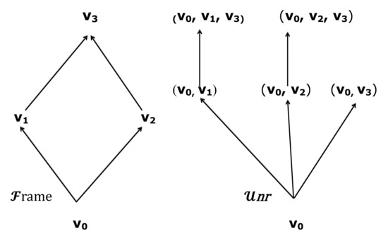 Figure 1. A Kripke frame (left) and an IBIS as its unraveling (right) [27].
 - 2.
- Simultaneously, the structure , where:= , , , , , ,is determined by the set, and and forms an example of an interval-based Kripke frame-based model extracted from IBIS in Figure 1 (right).
The concept of Kripke frames will be initially exploited for establishing a satisfaction relation for both ITL-formulae and HS-formulae in Figure 2. Finally, it will constitute a basis for the fibred models for our hybrid JusHSM.
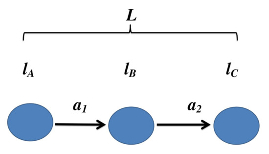
Figure 2.
An illustration of the IBIS-system from the example [27].
2.2. Simplified Interval Temporal Logic (SITL) and Halpern–Shoham Logic (HS)
The general remarks on the nature of Kripke frame-based semantics allow us to characterize both SITL and HS now.
I. Simplified Interval Temporal Logic of Moszkowski. ITL—defined in [4]—as a far modification of LTL of A. Pnueli— forms a highly expressive predicate modal-type representations of temporal relations that may be indicated between subintervals of a given interval. The relations next and semicolon constitutes the basis relations. They are used in defining further relations: begin, finish, halt, keep, yields, always, eventually, next (The full presentation of ITL may be easily found in [4]. Its presentation will be omitted for the brevity of this section and compactness of the analysis.).
In this paper, a simplified propositional variant of ITL of Moszkowski—the so-called Simplified ITL (SITL) is put forward. Introducing SITL we decide for a slight reconstruction modification of the original depiction of ITL from [4,5]. The foundation differences are the following:
- the uni-modal temporal operators of ITL restricted to begin, finish, halt, keep, always, eventually, next are admitted in syntax of SITL only (It means that we reject i.a. a bi-modal yield operator.),
- slightly against the original Moszkowski’s approach—the mutual relations between intervals and their subintervals are more explicitly given and considered as unique Kripke accessibility relations (Indeed, Moszkowski seems to consider these relations (different types of inclusions) as implicitly presupposed.).
Syntax ofSITL. Let us assume that form propositional variables, stands for ‘p semicolon q’(p followed by q) and let us adopt a couple of unique atomic formulae: true, empty, skip. Then the syntax of SITL-entities is given by the grammar:
where p, q are propositional variables, stands for: ‘generally in initial subintervals p’, stands for: ‘eventually in initial subintervals p’, stands for: ‘generally in terminal subintervals p’, stands for: ‘eventually in terminal subintervals p’. The pair: , stands for the intermediate subintervals, for: ‘next p’ and denotes a modal operator for X-relation, where . Some of the formulae are mutually co-definable. For example:
Meanwhile, the modal-type operators enable of defining some new operators introducing their co-definability and a piece of creativity inside SITL (see: [4], pp. 16–17) (This fact elucidates the concise presentation of the SITL grammar as given by (4) and (5)):
For example, (7) asserts that is true for intervals that terminate the first time the formula p is true. Thus ’halt’ can be thought of a forcing an interval to wait until p occurs [4], p. 17. (9) for ‘fin’ asserts that p holds for a terminal subinterval of length 0, i.e., for the interval’s final state. Their semantics will elucidate a more profound sense of the operators.
A deeper sense of the operators will be elucidated by their semantics.
Interval models for Simplified-ITL (SITL). Before we specify the semantic relations associated with the unary-modal SITL operator to deeper specify Kripke model-based semantics for SITL, we will be initially based on the definition of Kripke frame-based models for SITL as a triple: , where:
- W is a (non-empty) domain consisting of finite discrete intervals,
- V is a valuation, i.e., satisfying the usual conditions imposed on this function, and
- X is a relation between intervals from W and their subintervals to be called ‘Moszkowski’s relation’.
Let us establish now that I, denotes a proper subinterval of I consisting of the points up to for some , denotes a proper subinterval of I consisting of point from up to for some , etc.
If , M is an interval Kripke frame-based model, then—due to [4]—the satisfaction for the ITL-operators is introduced by the appropriate clauses as follows. (This definition collects and slightly reconstructs single conditions for satisfaction scattered over pp. 11—12,15,16 of [4].)
Definition 5.
(Satisfaction for SITL) Let us assume that an interval Kripke model M with a non-empty universe W and a discrete interval are given, for some fixed k. The following clauses define satisfaction relation for :
- 1.
- .
- 2.
- 3.
- ,
- 4.
- ,
- 5.
- .
- 6.
- ,
- 7.
- ,
- 8.
- ,
- 9.
- ,
The satisfaction conditions for other operators may be introduced via their syntactic co-definability with the operators just presented.
It is easy to see that satisfaction conditions from Definition 5 are not explicitly involved in accessibility relations between intervals—as usual in Kripke frame-based semantics. Nevertheless, it is not difficult to see that these relations (inclusions ⊆) may be easily extracted from the conditions. In fact, they are of a (slightly) different sort. The inclusions associated with operators will be denoted as and they connect intervals with their terminal subintervals. By contrast, the inclusions associated to operators will connect intervals with their initial subintervals and denoted by . Finally, the inclusions will be associated to and connect intervals with their intermediate intervals—due to the satisfaction condition for these operators. Finally, we can venture to name some chosen relations. Namely, will be semantic counterpart of SITL operators: fin, keep, halt, beg (We decide to treat them here as modal operators—as we think about them as about fin(), keep(), halt(), beg(). If a propositional variable is fixed, say p, then the corresponding fin(p), keep(p), halt(p), beg(p) are unary predicates.) (resp.) These arrangements lead to the unitary and generalized satisfaction condition:
for , and being a diamond-type unary operator of (SITL). The corresponding condition for operator requires a general quantifier instead of the existential one.
II. Halpern–Shoham logic. Whereas ITL and its simplified version SITL are capable of rendering the internal relations inside a given temporal interval (between its inherits fragments), HS renders external relations between a given interval and other intervals.
Syntax. More precisely, HS constitutes a modal-type representation of temporal relations between intervals, originally defined in [6]: “after” (or “meets”), (“later”), “begins” (or “start”), (“during”), “end” and “overlap”; see also [7]. These relations correspond to the modal HS operators: for “after”, for “begins”, for “later”, etc. The syntax of HS entities is defined by:
where p is a propositional variable and denotes a modal operator for the inverse relation w. r. t. being a set of Allen’s relations.
Semantics. As earlier mentioned—the appropriate semantics of HS forms a kind of the interval-based semantics. Denoting by the set of all closed intervals for , the interval HS-model is defined as n-tuple , where and is a valuation for propositional letters of .
Sometimes, the interval-based models for HS base on generalized Kripke frames, i.e., on the triples of a more general form , where W is a (non-empty) domain, V is a valuation (Alternatively, we can define the corresponding IBIS-based model provided that we exchange a valuation V for a labeling function.) and . If , M is a Kripke frame-based model of this type, and , then satisfaction for ⋄-type modal HS operator is given as follows:
Exchanging ∃-quantifier for the general one, we can obtain the corresponding condition for □-type modal operator.
Example 3.
Let M be a Kripke model, are two interval from the model universe and forms an exemplary predicate of a given propositional modal language . Then
3. A (Simplified) Halpern–Shoham–Moszkowski Logic
Having defined both SITL and HS, we are in a position to propose an integrated temporal logic system to be called Halpern–Shoham–Moszkowski logic (shortly: HSM). In this section, HSM is introduced syntactically only—as a complex presentation of its semantics requires a new combined type of semantics to interpret combined formulae of HSM. It will be elaborated in Section 5 as the so-called fibred semantics, and it will be retrospectively adopted to HSM formulae.
It arises a question how to combine these two systems. It seems that the most simple and (perhaps) the most natural way to do it is to consider their fusion (or an independent sum). Generally, if are two modal logics in languages (resp.) and they have disjoint sets of modal operators, say and (resp.), then the fusion
of and is the smallest ()-modal logic containing both and .
Therefore, let us assume that a new language being a fusion of and . Nevertheless, we intend to admit some combined formulae of ITL and HS, thus the new HSM should constitute a kind of superset of a usual fusion . In other words, a set of well-formed formulae of , say , should contain the set =: either FOR or FOR as its proper subset.
Nevertheless, not all combinations should be admitted because of a nature of the scenario from the motivating example (see: Introduction), which indicates the admissible order of the modal operators of HMS. Namely, HS operators play the role of the external operators for the ITL’s ones. In fact, the situation should be initially described inside a given interval, and—eventually—its materialization may be moved in time (performed in another interval provided that it remains in the initial one in Allen’s relation).
It allows us to define a set of well-formed formulae FOR of HSM in .
Definition 6.
(Set of well-formed formulae of HSM) A set FOR of well-formed formulae of HSM is given by the following grammar:
where are propositional variables and , is ‘next’-operator and and are mutually co-definable temporal operators ’eventually’ and ’always’ for and is an Allen’s relation.
Example 4.
The formula: finϕ is a well-formed formula of HSM, but halt—does not.
Definition 7.
(HSM as a theory) HSM is defined as the smallest theory containing all formulae FOR and closed on MP, substitution, and the corresponding inference rules for formulae of ITL and HS.
4. Multi-Valued Verifiability Logic (MVer)
4.1. Towards a Multi-Valued Logic for Gradable Verifiability
Before we propose the fibred semantics for combined formulae of HSM already introduced, we need to elaborate at first a multi-valued logic for gradable verifiability (MVer) to integrate it with HSM. In this way, the hybrid VerHSM will be introduced.
In this section, the lacking component MVer will be elaborated. In general, we intend to adopt the formalization tradition for the close-related concept of provability in terms of Löb-style modal conditions (see: Introduction). Comments of Ayer, Chisholm, and Gettier regarding the justification as an epistemic capability of agents from [28,29,30] will determine the final exploration direction.
Towards a Basis Verifiability Logic. It remains to decide which modal logic system should be adopted as a basis system for the verifiability logic construction. In order to find the most reasonable solution, we now consider three candidates aspiring to this role.
The first—and potentially the most natural—candidate seems to be the Gödel–Löb logic GL which expresses Löb’s provability conditions for Gödel’s incompleteness theorem in terms of □-modal operators. The following axioms K, 4 and GL determine its axiomatic system—as already mentioned in the Introduction—:
- K ,
- 4 ,
- GL .
Independently of this concise modal representation of provability in the axiom-based framework of GL logic—it remains some difficulty with the naturality and universality of the third condition. Indeed, one can argue that it has a relatively narrow and technical sense (for the use of the proof of Gödel’s theorem), and it should not be easily extrapolated for a broader spectrum of contexts.
The concurrent solution in the same formalization approach to arithmetic provability oscillates around its representation by formal properties of Prov()-predicate given by the so-called Rosser’s sentence (see: [31,32]), the chronologically second metalogical example of an undecidable Gödel’s sentence.
It asserts—as a self-referential sentence—that if it has proof in PA with a Gödel number k, then its negation has a proof in PA with a Gödel number m smaller than k (In fact, it forms a roundabout method for this sentence to state its own non-provability. The predicate version of the sentence may be found in [31]—due to the original one from [32]. We omit its presentation because it is redundant from our perspective.). In this way, provability was explicitly combined with a time sequence relation in Rosser’s trick for his Gödel sentence construction and his concept of provability in general. On the one hand, an idea to exploit Rosser’s sense of provability in our approach seems to well correspond to our main idea of combining verifiability with time. On the other hand, there is no explicit axiomatic depiction of provability involved in Rosser’s sentence— even against a promising effort of Smullyan to give Rosser’s sentence an epistemic face. He made it in terms of a belief operator B (If is an atomic, self-referential sentence:’I am provable in PA’, ’<’ is the time sequence relation, then the Rosser’s sentence may be identified with BB (I am provable only if you cannot believe that I am provable earlier than you believe that I am not provable).). In addition, Smullyan’s approach forms a taxonomy of axiom systems dependently on agent epistemic capabilities established a priori (such as agent-Besserwisser, an epistemically naive agent, etc.) Meanwhile, we rather intend to find an axiom system for describing formal properties of (gradable) verifiability itself, while the agent’s epistemic capabilities may be flexible and context-dependent such as reasoning about digital circuits.
Returning to the formalization approach in terms of GL, it seems to be reasonable to exchange the technical axiom GL for a more general axiom T: ‘if A is justifiable, then it is true’ in our approach. Indeed, this axiom much better materializes an idea of the truth assignment to different logical statements based on an acceptance of their premises. It leads to the exchange of axioms: K, 4, and GL for the conjunction of K, 4, and T. In this way, GL will be exchanged for S4—as a basis for further constructions. It forces some conditions imposed on the semantics of the newly introduced MVer—because S4 is complete w. r. t. the models based on the partially ordered Kripke frames (Obviously, S4 adequately describes (in the sense of completeness) not only partially ordered structures, but also such entities as dense-in-itself metric spaces ([33]), etc. Nevertheless, this “unintended” S4-semantics will not concern us as redundant and inadequate.).
Multi-Valued Logic for Gradable Verifiability. It only remains the question of how to modify the epistemic S4 to make it suitable to represent gradable verifiability in order to define MVer. In order to do it—let us introduce a finite set of different parameters in a role of degrees of ‘being verifiable’. More precisely, we will admit new parametrized modal operators of the type: (for: ‘ is justifiable by an agent i with a degree ), where is an ordinary box-type operator read: ‘ is justifiable’). It is convenient to treat the -parameters as normalized, i.e., . Since a finite set of such ’s degrees is usually enough in practice, this new MVer will form a multi-valued logic system (Let us note that even such an extremal case as ( is justifiable by i in the degree 0) does not violate our meta-assumption concerning a purely descriptive character of our system, we consider this case as acceptable.). Summing up, we intend to identify MVer with a multi-valued epistemic S4.
4.2. Multi-Valued Epistemic Logic (MVJus)—A Syntactic Depiction
These postulates—just formulated—will find their reflection in syntax of MVer by introducing the following two modal operators:
- 1.
- for: ‘ is (strongly) justifiable by an agent i with a degree ’ and
- 2.
- , for: ‘ is (weakly) justifiably by an agent i with a degree ’,
for atomic and an arbitrary, but fixed rational parameter —due to [34,35]. It allows us to establish a grammar of MVer as follows.
Language of MVer. Let G be an arbitrary, but fixed finite subset of (parameters from) . The language of MVer, (MVer), is given by the following grammar:
where , is an arbitrary, but fixed rational parameter from G. The following definition establishing a co-definability of modal operators of MVer and the following axioms are incorporated in the syntax of MVer.
Def. 1: for each .
Axioms:
- 1.
- All axioms of Boolean propositional calculus,
- 2.
- , (axiom K)
- 3.
- , (axiom 4)
- 4.
- , (axiom T)
for each fixed rational .
Inference rules: As inference rules we adopt:
- 1.
- Modus Ponens, substitution rule and
- 2.
- a neccessitation rule for the -operator:
rational and G finite. It allows us to define MVer as a formal theory in the following manner.
Definition 8.
(MVer as a theory) MVer forms the minor theory in , which contains: Definition 1, axioms (1)—(4) and closed under the inference rules, mentioned above.
Example 5.
Let us consider an atomic formula of an atomic ITL-formulae and consider an agent , and . Then:
- 1.
- is well-formed exemplification of axiom T, but—for
- 2.
- does not because we admit α as fixed during for the whole formula construction only.
4.3. Interval-Based Semantics for MVer
In this paragraph, MVer will be interpreted in Kripke interval-based semantics. As usual, a “core” of its construction is a two-stage construction the appropriate accessibility relation between intervals (for ). This relation is intended to constitute a non-symmetric similarity relation (Let us note that a usual similarity (as a purely qualitative) relation is an equivalence relation. Indeed, it is reflexive, symmetric, and transitive. Nevertheless, if we are interested in a numeric scale of similarity—this relation violates symmetry. This fact suggests us a research direction. Indeed, we will specify numerically.) and partially have a pragmatic nature (as agents index it) to introduce a piece of behavioral semantics. Additionally, this relation will be specified later by ’s in the construction’s next-stage – due to some ideas previously eleborated in [27,36].
Accessibility relation . For defining this accessibility relation let S be an initial (reservoir) set of finite intervals (Pedantically, S might be defined as a power set of all finite sequences of points taken from a non-empty W. For simplicity of current analysis we omit this initial stage of the construction.), and let the intervals , and , for some . Let us also establish an agent and let us define a new accessibility relation between intervals I and as follows:
i.e., an agent i cannot distinguish between the corresponding states of I and up to j state, between j-prefixes of both intervals. In other words,
or if and only if the behavioral equivalence condition (see: Section 2) holds for j-prefixes of these two intervals.
It is not easy to show that forms a partial order, i.e., it is reflexive, anti-symmetric, and transitive, for each . Thus, it forms an adequate relation for Kripke models for S4.
Theorem 1.
The relation defined by (12) forms a partial order, for each .
Proof.
Let us establish an agent . It is clear that , so the relation is reflexive.
If assume that two I and are arbitrarily chosen and such that length(I) = k, length( and , then and it is not true that (for all such pairs). Thus, it cannot hold —due to (12) in a general case. Obviously, if symmetry holds, then . Hence, is anti-symmetric.
If and are such that length(, and and , then also-due to (12) — and and , for all . It exactly means that , i.e., is also transitive for the fixed . The thesis of Theorem follows from the fact that was chosen arbitrarily. □
Accessibility relation . Obviously, relation is not suitable to grasp gradable verifiability by agents. In order to empower for this task, we should modify this relation. Therefore, let us establish a finite and let us consider some technical function defined as:
Intuitively, this new function associates the earlier relation between I and to some rational from (The appropriate methods of achieving of will be discussed later.). We are in a position to introduce a new relation in the product as a unique enhancement of the previous as follows:
Obviously, this general way of defining does not determine its nature precisely. Its algebraic properties depends on a method how is defined. However, this way of introducing allows us to preserve some crucial properties of such as anti-symmetry. It follows from the condition length( length () for a given pair of intervals I and (In fact, if for intervals I and and some , then length( length () and the inverse inequality does not hold (in a general case), thus it is not true that also . It already disconfirms symmetry.).
The following example (Figure 3) illustrates now how a way of defining influences an algebraic nature of .
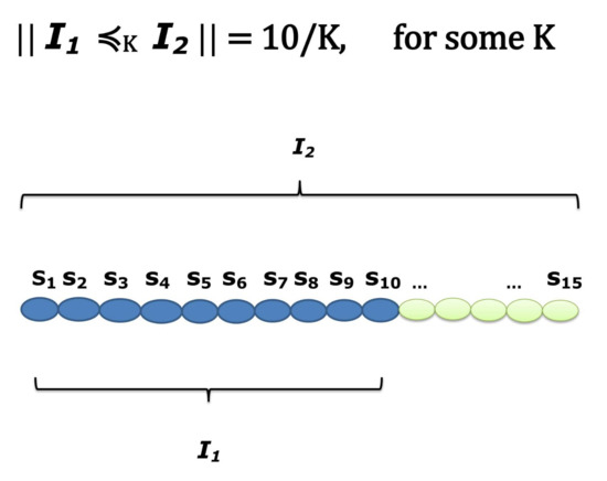
Figure 3.
Two intervals with a common prefix and their behavioral similarity [27].
Example 6.
Consider a pair of discrete intervals having common points and define for some length of each interval and each . Thus, their similarity . Assuming that we always obtain by this way of establishing α. In fact, we always find an α value no greater than 1 (because of a denominator = 200) and . (It there is no common point we obtain 0). Obviously, , thus this way of defining α also preserves transitivity.
Having defined , we are in a position to define a Kripke interval model for .
Definition 9.
(Kripke model for MVer) Let be a non-empty set of agents. A Kripke interval model for MVer associated to is each structure M of the form:
where , is an accessibility relation on and is a truth assignment function (As usual, we treat the assignment function as an extension of a valuation function running from a set of propositional variables to a a family of subsets of S. We decide for such a slight modification because of further analysis around fibred semantics, where usually assignments are considered instead of valuation functions.).
It allows us to introduce the following inductive definition of satisfaction for MVer-formulae.
Definition 10.
(Satisfaction) Let be a Kripke interval model associated to a non-empty set for with a set of propositions . Given a formula (MVer), an interval and a finite set we inductively define the fact that ϕ is satisfied in M, in an interval I (symb.) as follows (It is easy to reformulate this definition for satisfaction in the corresponding IBIS system. In fact, it is enough to exchange the initial condition for atomic formulae from Prop for the condition: for all , we have IBIS, iff .):
- 1.
- For all , we have iff .
- 2.
- iff it is not such that .
- 3.
- iff and .
- 4.
- , where , iff for all we have for each .
- 5.
- , where , iff there is such that and for each .
The key clauses in this definition are that one referring to the modal operators and . These conditions assert that these formulas are satisfied in I of M iff the atomic formula holds in all intervals (at least one interval) accessible from this I via -relation (resp.).
It remains to reconcile syntax of MVer with its semantics given by Kripke interval models as defined in (14)—at least in the form of soundness (The proof of completeness would require more detailed analysis and the construction of the appropriate canonical models.). It means that all formulae MVer are satisfied in Kripke models of this type.
Theorem 2.
(Soundness of MVer) Theory MVer is sound with respect to all Kripke interval models with accessibility relation defined by (13), for each and fixed rational .
Proof.
For the established and the parameter the proof runs as in a standard way for classical model logic systems. One needs to show that all axioms K, 4, and T are satisfied in Kripke models defined by (14). In order to illustrate, we consider axiom T only.
Therefore, let us assume that is such a Kripke model associated to and and Prop. Let us establish an agent and and assume that . Then—for all we have . In particular, —because is reflexive, thus . It exactly means that , i.e., for the fixed and . Since both and were chosen arbitrarily, for all ’s and i’s. □
In this way, a Kripke frame-based interval semantics was determined for MVer. It will be exploited as a component of the fibred semantics for the hybrid MVHSM.
5. Multi-Valued Simplified Interval Temporal Logic (MVHSM)
Having elaborated the appropriate conceptual apparatus to combine MVer with HSM, we are in a position to introduce the hybrid MVHSM. It will be suitable to grasp not only the gradable verifiability (like MVer), but also temporal relations between intervals of the external nature (like HS) and the internal one (as ITL). One needs to underline that MVHSM constitutes more a reservoir of its possible subsystems than a complete axiomatic formal system. In this sense, its construction preserves the nature of both HS and ITL, which should be viewed in a similar way.
5.1. Syntax of MVHSM
As previously, a usual fusion cannot constitute a construction basis for MVHSM. It follows from the requirements to admit different combinations of MVer-formulae with HSM-formulae. Meanwhile, the nature of Formula (3) from the motivating example delivers a coupe of potentially useful guidelines on how to combine these two systems.
- *
- modal operators of MVer should be the most external in the combined formulae of MVHSM,
- **
- modal-temporal operators of HS should be internal with respect to the MVer operators but external with respect to modal-temporal operators of ITL.
To cut a long story short, ITL-operators should be the most internal, MVer-operators should be the most external.
We will define a set of well-formed formulae of MVHSM, say , in a language being a fusion language, i.e.,
Before of a variety of temporal and epistemic components in —it is reasonable to briefly specify a taxonomy of possible subformulae of . Starting from the less complicated ones, one can indicate the following classes of them:
- atomic:
- all atomic formulae of each subsystem: HS, ITL and MVer taken cumulatively,
- unimodal:
- all unimodal formulae of HS, of ITL and of MVer taken cumulatively,
- bimodal:
- all formulae with two modal operators in different configurations: MVer-modal formulae combined with ITL-modal formulae, MVer-modal formulae combined with HS modal formulae and HS-modal formulae combined with ITL formulae—due to combination principles * and **.
- trimodal:
- all formulae with three modal operators of MVer, HS, and ITL combined due to combination principles * and **.
It leads to the following definition of (Although the unimodal ITL-operators keep(p), halt(p), beg(p), fin(p) are not distinguished in the grammar of SITL explicitly—we treat them as explicit unimodal operators in the definition of because of their practical importance. In addition, they are definable by unimodal operators and , for .).
Definition 11.
() Let α’s and and let be defined as in (15). Then a set FOR of well-formed formulae of is given by the following grammar based on the following taxonomy of types of formulae:
where are a propositional variable, , where is a set of agents, and , is ‘next’-operator and and are mutually co-definable temporal operators ‘eventually’ and ‘always’ for . Finally, is an Allen’s relation.
By analogy, MVHSM is defined as the most minor theory in containing all formulae FOR and closed on Modus Ponens, substitution and the corresponding inference rules for formulae of MVer and HSM.
Example 7.
- 1.
- The formula fin(ϕ) belongs to FOR for , , but
- 2.
- does not, for and because the order is prohibited by the syntax of MVHSM.
5.2. Semantics for Uni-Modal Formulae of MVHSM
Having defined the syntax of MVHSM, we will propose a complex frame of a semantic interpretation of this formal hybrid system. Due to previous establishments—we will make staring from uni-modal formulae of . Indeed, the semantic interpretation of uni-modal formulae of has already been introduced when each of the components of MVHSM was characterized. Therefore, the role of this subsection is to propose a slight generalization of previous analysis concerning semantics for these components. It is especially crucial for SITL in order to elaborate a coherent facon de parler before introducing the so-called fibred semantics for combined formulae of MVHSM.
In order to elaborate this general glance into semantics for uni-modal SITL-formulae, let us return to satisfaction conditions for HS logic. If a Kripke frame , for being an Allen’s relation, is given and , then
- (1)
- iff there is such an interval that ( and ) and
- (2)
- iff for all intervals that ( and ).
The corresponding generalized conditions for satisfaction relation for SITL-formulae should be sensitive to the nature of interval relations described by SITL. It is easy to observed that we deal with the same scheme of an initial interval and its subintervals independently of the type of relation. We can also put aside the nature of these intervals (In fact, it is no matter whether they are discrete or continuous. They should only form subintervals of the initial one.). However, we can venture to divide all SITL relations into two classes.
The first class contains explicit ⋄- and □-type operators , for . Let us denote them collectively for the use of this section’s analysis by and . The second class contains a couple of distinguished relations of an implicitly modal nature (because of conditions (7)–(9)). As observed previously in Section 2, different semantic conditions determine satisfaction for these two classes of SITL modal formulae. This fact finds its reflection in the following generalized satisfaction conditions for SITL-formulae.
Let us assume that a similar Kripke frame , for , and , then
- 1.
- iff there is such an interval that ( and and and
- 2.
- iff for all intervals that ( and and ,
where * is either T or I.
Obviously, dependently on the relation, ⊆ is a unique type. For ’halt’—because of its representation in terms of operator—we deal with . ‘Finish’ is referred to (1) because fin is defined by operator (see: condition (9)).
Let us assume now that a Kripke frame , for , and , then
- 1.
- iff there is such an interval that ( and and
- 2.
- iff for all intervals that ( and ,
where .
For establishing a corresponding more general Kripke interval model for the fusion MVer⊗HSM (Let us repeat that the fusion does not contain combined formulae.)—it remains to define the appropriate assignment function (MVer⊗ ITL) for each modal operator (of this fusion language). It is convenient to define h inductively as follows.
Definition 12.
(A truth assignment for ) Let be a Kripke frame with accessibility relations: , for , defined as earlier, X as a SITL-relation and Y—an Allen’s relation, for . Then the function (MVer⊗ ITL) satisfying the following condition:
- 1.
- , for ϕ atomic,
- 2.
- ,
- 3.
- , for * is either I or T.
- 4.
- , for ,
- 5.
- .
(For the diamond operators, we exchange general quantifiers for the existential ones.) is said to be an assignment for the fusion language .
It allows us to define Kripke interval models for the fusion language . For simplicity of further analysis, let us establish a single symbol for an arbitrary SITL relation (Moszkowski’s relation) being either X relation () or an accessibility relation . They will be simply called ’SITL relations’.
Definition 13.
(Kripke interval model for ) A Kripke interval model associated to for is each structure of the form:
where, for each :
- is a model universe consisting of finite intervals (Let us note that we do not specify how the intervals are obtained and what is their nature (discrete or continuous). Paradoxically, it allows us to simplify the definition by considering a common model universe S as a reservoir of all integrals, so we decided for such a solution. It may be problematic for fibred models, where combined formulae are interpreted.),
- is defined by (13), is a SITL-relation, Y—an Allen’s relation,
- h is a truth assignment function defined as in Definition 12.
Obviously, all the relations , relations ’s and Y’s relations of Allen are accessibility relations between intervals. If a Kripke frame, say , is given, then a Kripke interval model (over ) forms a pair , where h is a truth assignment defined as previously.
Finally, one could also distinguish Kripke interval models for the components and taken separately. Thus, let us assume that and and are Kripke frames for MVer, SITL and HS (resp.), i.e., , for and as previously, , where is a SITL relation, and , where Y is an Allen’s relation. In order to create Kripke models from them, it is enough to establish the corresponding assignments: (resp.) — each of them obtained from h assignment restricted to the appropriate sets of formulae. Hence, , , and .
5.3. Fibred Semantics for Combined Formulae of MVHSM
It is easy to see that Kripke interval models, such as , or above, are not suitable for combined formulae. In fact, they are adapted to interpret uni-modal formulae of the MVHSM system only. One can expect that a remedy for this difficulty might be the appropriate form of the so-called fibred semantics (The fibred semantics is alternatively called ‘fibring semantics.’)—recently described for a point-wise semantics by D. Gabbay and V. Shehtman in [24]. The founding idea of fibred semantics itself may be informally expressed as follows. If you cannot interpret a combined multi-modal formula of a given language in a model, say (i.e., cannot properly ‘recognize’ this formula), then:
- find models, in which may be interpreted (they can properly recognize this formula) and
- built a connection between these models and the initial model and
- accept that if is satisfied in all these models, it is also satisfied in itself.
In this subsection, we shall demonstrate how the mechanism of the fibred semantics works for combined modalities of MVHSM, which cannot single models cannot model. Hence, we intend to propose an extrapolation reconstruction of Gabbay’s fibred semantics for the interval-based semantics. In more formal terms, the main idea of fibred semantics for interval-based semantics will be as follows.
I. The frame of fibred semantics for interval-based semantics. Let us assume that a modal-language (Let us note that we do not impose any restriction on to be a multi-modal language.), and let be a Kripke interval model for with a universe S. Let also assume that we intend to evaluate a modal-type formula (dually: ) of another modal language, say . Let us assume that , i.e., cannot usually interpret as it cannot properly ‘recognize’ it (as the modal formula with □-operator).
In order to make the problem decidable-we empower the model to be capable of interpreting as follows.
- 1.
- Establish an interval, say , from ’s universe S,
- 2.
- Associate to a new pair , for ( is parametrized by ).
- 3.
- If it is possible—associate to each such pair that , for . In other words, for a given interval from a model , establish a fibring mapping F: ), for some natural k.
- 4.
- Establish finally a new (conditional) satisfiability for in as follows:for as above.
Since F: ), one can reformulate condition (17) to the following one:
for as previously.
Being equipped with the new formal machinery to interpret combined formulae, we can return to our motivating example, where an agent’s epistemic behavior during its supervision of the loading phase in digital circuits was described by Formula (3).
We intend to interpret the combined multi-modal components of this formula semantically.
The Motivating Example 1.
Let us return to the situation of our agent supervising some fragment of ‘loading phase’ action. It has been established that the statement: “An agent i verifies with a degree α that always later (the situation): ‘initially was H and finally’ status=1” occurred” may be rendered by the combined multi-modal Formula (3):
Illustrate how to semantically model the combined multi-modal formula:
(For simplicity of explanation, we decide to avoid the second internal atomic subformula . Obviously, it does not change the interpretation approach.).
Solution.0.Pre-processing: Let us consider a (slightly more general) formula fin(, where is an arbitrary HS-modal operator. Obviously, —due to Definition 11. We should establish the initial modeling situation as coherent with the procedure of the fibred semantics construction now. Thus, let be a model (of a universe S) not capable of recognizing as a tri-modal formula of . In other words, interprets not as fin( (with atomic), but as a unimodal (with fin( as atomic).
Because of the complexity of further construction of fibred semantics must be two-stage. In the first stage, we empower to correctly recognize the next external modal HS-operator . In the second one, we deliver the model a capability to recognize ITL-operator fin.
1. Stage. Due to points (2) of the construction algorithm—we need to establish a fibring mapping F between and a new model (of a universe ) to overcome the incapability of to properly interpret(evaluate) fin as bi-model formula. It allows us to ‘transfer’ the validity checking from to the validity checking within the second one. We do it for the most external HS-operator of this subformula (For simplicity of considerations, let us consider a single model only.).
Thus, let us establish an interval and associate to a new pair , for via the fibring mapping F such that: F.
Due to point (4) of the construction algorithm—let us establish the (conditional) satisfiability for in model , for -as atomic for this model, as follows:
2. Stage. Although can evaluate HS-formulae ( can already do it, too), it may not recognize fin as bi-modal formula. In other words, it may ‘see’ fin() as a formula of the form only, where q is atomic. Hence, we should repeat the same reasoning for and associate a new class of models, which are in a position to normally evaluate SITL-formulae. For simplicity—as previously—let us consider a single model only, say , and establish the following new satisfaction condition in for fin:
(Note that F(F is a new interval in associated to via F —as was associated to via F. Thus, we need a doubleF.)
Summing up: the tri-modal formula may be evaluated in because of supporting models (where HS-subformula is evaluated) and (where SITL-subformula may be evaluated) and their connections with by means of fibred mapping F (Here and in each place later, we will understand the fibring mapping F as a mapping completely determined by conditions (3) and (4) of the fibred semantics construction. Therefore, we do not impose any restrictive limitations on it. However, it is sometimes convenient to adopt the “switching condition” for F: for each , it holds F and for each : F. Finally, if , than also F—due to [24]. Let us note that F must not necessarily be a function.).
Establishing this condition finishes the procedure. In many cases.
II. The fibred Kripke models.
Having described a construction frame of interval fibred semantics, we can venture to introduce a detailed definition of fibred Kripke models for MVHSM on a base of the models earlier introduced. All components of this logic system should be considered. Since we want to preserve information about the initial provenance of all components in the new model (about domains, relations, and assignment functions), we venture to exploit an algebraic concept of a simple sum in its definition. Because of the unique role of fibring mappings in the evaluation process, they will be singled out as separate components of the fibred Kripke models.
It leads to the following definition of the fibred Kripke model.
Definition 14.
(fibred Kripke model) Let us assume that , and are the interval-based Kripke models for HS-componant, SITL-component and MVer-component of MVHSM (resp.). More precisely, let us assume that:
- 1.
- , , for some fixed (In general, , but we can also accept or or even . Finally, it is also acceptable to take , and as denumerable sets of finite sequences (intervals). We decide for their finite cardinalities for clarity of their presentation.).
- 2.
- is a SITL relation, Y is an Allen’s relation and is a similarity relation as defined by (13), for , and
- 3.
- , , form assignment functions in and (resp.),
- 4.
- Fis a fibring mapping.
Then a fibred models for MVHSM is the following tuple:
where ⊗ denotes a simple sum the appropriate components.
5.4. The Scenario from Motivating Example in the Fibred Kripke Models
Having explored principles of fibred semantics for different components of MVHSM, let us illustrate its mechanism for the tri-modal formula from the motivating example:
It is reasonable to start with Kripke models for uni-modal subformulae of (22) to propose a fibred Kripke model for the whole formula.
Model for epistemic MVer-component of the formula. In order to find a model for the epistemic (outer) component for (22)—let us assume that and are two intervals interpreting the verification capability of agenti such that:
- is an interval where this capability to verify the situation that ‘fin’ is expressed and
- is the interval, in which the situation described by fin holds.
Formally: (Note that may not recognize the formula properly. It illustrates a need to consider a fibring mapping in the hybrid model.). Assume also that is an accessibility relation between them, i.e., it holds . Thus, a model for the epistemic component is given as follows:
for some valuation for epistemic MVer-formulae.
Model for the HS-temporal component. Our task is to find a model for HS-temporal component now. Therefore, let us consider two temporal intervals:
- for representation of “now” (it may be a singleton) and,
- for representation of ”sometimes in a future”.
As previously,
- 1.
- is the interval, where the situation described by fin is expressed,
- 2.
- is that interval, in which the simplified situation ’fin holds.
Formally: fin (Note that may not recognize the ‘fin’ operator, so it forces a need to consider a fibring mapping and a new supporting model, which is already capable of doing it.).Thus—if L represents Allen’s ‘later’-relation—the appropriate model for HS-component of (22) is given by the tuple:
for some assignment for HS-formulae.
Model for the SITL-temporal component. In the similar way, we are in a position to find a model for SITL-temporal component. Because the situation described by ‘fin’ we need the following pair of intervals:
- J, where ‘fin is expressed and
- as a final subinterval of J, where ‘status = 1’ holds
The appropriate model for SITL-component of (22) is the tuple:
for some assignment for SITL-formulae.
The previous constructions of the fibred model components lead to the depiction of whole fibred model for the Formula (19) as the following tuple:
where:
- ,
- ,
- F is a fibring mapping (By default, F connects with , and with .).
In this way, the Formula (19) describing a piece of agent reasoning about digital circuits found is a semantic reflection in fibred Kripke semantics for the MVHSM system.
6. In a Broader Context of the Model Checking Problem
Although the logical approach to reasoning about digital circuits has a prototype character, it seems reasonable to locate it from a broader perspective.
6.1. The Paper Ideas and Research on Digital Circuits
It has been already said that ITL from [4] found its application in a formal representation of different digital circuits of the arithmetic and combinational type, such as adders (see: [4], pp. 55–64) or multipliers (see: [4], pp. 86–88). The formal apparatus of ITL may also be exploited for the use of formal representing the data handling combinational circuits, such as Multiplexer (see: [4], pp. 86–88) and many others. Obviously, the ITL formulae describing the behavior and properties of these computational circuits—as unique formulae of (an appropriate description-logic based extension of MVHSM)—may be interpreted in the Kripke interval models just proposed. It is noteworthy that the unary specific predicate —exploited in our motivating example—supports a formal representation of the behavior of other types of data-handling computational circuits, such as Implementation (close related to Multiplier)—due to definition ( is defined as previously in the paper body, and is defined in the following way.
Due to—[4], p. 109—a behaviour of ’MultiPhase’ may be explained as follows. When the load signal is inactive at 0 () and the device has Status=1 (is steady), the circuit can be clocked to perform a single iteration. The algorithm’s predicate runs over two clock cycles. Afterwards, the device is always again steady with Status equaling 1 ([4] p. 109)):
Its behaviour should be understood as follows. The device’s fields are shown by lmpStructure. The predicate LoadPhase specifics device operation for initially loading the inputs. Once this is achieved, the predicate MultiPhase indicates how to perform the individual multiplication steps (see: [4], p. 107.) Obviously, one can also imagine the situation of much more complicated formulae of (an appropriate extension of MVHSM) to be capable of rendering the constitutive behavioral properties of many other digital circuits. The fibred semantics-just elaborated—delivers us a general frame for their semantic interpretation.
A natural question arises: how to refer the ideas to the newest types of digital circuits. They are usually represented by a broad spectrum of processors, microprocessors, or sophisticated flip-flop-based registers and designed due to limitations and deeply explored capabilities of VHDL specification. They form a far enhancement of the classical and basic digital circuits as adders, counters, or single flip-flops. (See: [37].) It seems that its sophisticated nature might elude the formalization efforts, such as in terms of MVHSM and its appropriate extensions. Meanwhile, a deeper look at the development tendencies in research on digital circuits delivers a piece of optimism in this matter. Indeed, they include such research trends as estimating and reducing resource usage, producing faster circuits, improving processor performance, etc. It seems that these deeply engineering problems and issues do not essentially impose any new restrictions on our formalization attempt concerning the initial Moszkowski’s ones from [4,5] for (at least two reasons). First, they have another semantic field, and they require another non-logic-based methodology to be solved. Secondly, our approach suggests how to move from formal modeling of basic circuits (such as single flip-flops) to modeling their multi-collections (such as processors). We need a mapping-based connection between our transition systems (of Kripke models for verification of circuit’s properties), which preserve the appropriate portion of information moving between the transition systems. Obviously, the small outline of the fibred semantics should be complemented by purely engineering requirements (f.e. imposed on the fibred mappings) to aspire to be a realistic fibred transition system (as a model) for some of the more advanced circuits. Indeed, the transitions system seems to be even more convenient in this role than interval Kripke models. It follows from the fact that they better grasp the internal dynamism of the devices. In addition, they seem to be a convenient semantic ‘mediator’ between a purely logical system of temporal logic such as , -calculus, ITL, HS, MVHSM, etc., and the purely declarative description languages such as HDS or VHDL.
Nevertheless, one needs to underline that no of these formal languages (even some extensions of MVHSM) can aspire to exchange the specification languages. Indeed, they play slightly another role. The main predestination of the specification languages is a synthesis-based creation of electronic systems. Meanwhile, temporal logic systems—due [4,7,16,17,18,38]—should be rather suitable (in the context of digital circuits analysis) for a formal description of different (external or internal) properties of them (such as liveness, lack of deadlock, the appropriate action sequencing). Models of these systems—even if they form transition systems and try to model digital circuits themselves—introduce a piece of an idealization and are more suitable for being well-founded in a mathematical sense. Thanks to this, they potentially form a convenient bridgehead for incorporating a piece of model checking machinery. It seems that some reference to these models (such as fibred models for MVHSM) is necessary if we intend to formally verify some properties of the modern digital circuits (such as processors) even if they have better ‘operative’ and algorithm-based depiction in terms of VHDL/Python interpreter. Some illustration how the model-checking machinery may be incorporated into the pipelined processor model—expressed in DLX assembly code—may be found in [23].
6.2. A Potential Benefit: Combined Model Checking
Indeed, this model-theoretic perspective of our (deceptively pure) logical approach is the model checking-oriented. Namely, in a conceptual frame of our combined logic-based approach, the model checking machinery for digital circuit’s behaviour and description may be integrated with model checking for pieces of reasoning about them. Even though our combined Formula (22) forms a simplified case of many other combined formulae for a description of many realistic scenarios of reasoning about digital circuits, its fibred semantics-based modeling illustrates some new possibilities of formal verification for many other similarly combined formulae. It seems to constitute a piece of novelty of the paper in the model checking immersed in electronics-based application contexts—even if the digital circuit properties’s and behaviour’s description—f.e. against the bounded model checking for microprocessors as in [23]—does not form a leading tendency in model checking speculations for electronics-determined application contexts.
Meanwhile, the general scheme of the model-checking procedures for MVHSM (and its potential extensions) may be given by the following algorithm.
The core of the algorithm is VERIFY function, which returns Boolean (true or false) for a given Kripke model (transition system), an interval and a given formula of MVHSM. For combined formulae, VERIFY also depends on fibring function F. It enables of verifying these formulae, which cannot be evaluated in initial models. This algorithm ellucidates at least tow benefits from incorporating the interval fibred semantics to model checking for properties of digital circuits. First, we can integrate a machinery of model checking for properties of digital circuits themselves with model checking for (formally depicted) pieces of reasoning about them (lines 22–25 of Algorithm 1). It draws some new perspectives—also in the area of automated model checking. Secondly, fibred semantics makes the whole model checking for MVHSM formulae decidable as it ensures the required connections between models. Meanwhile, the number of the procedure steps is finite (there is always a finite number of intervals to check, a set G of ’s is also finite).
| Algorithm 1:Model checking for MVHSM. |
|
7. The Results between Other Concepts
The paper analysis stems from research on interval temporal logic-both its theoretic and application-based aspects. The chronologically first and complex formalization approach to interval temporal logic found its reflection in Interval Temporal Logic of B. Moszkowski from [4,5] as a synthetic depiction of previous and context-dependent attempts from [1,2,3]. In this sense, Moszkowski’s system plays a role similar to the so-called Linear Temporal Logic—as a tense logic initially adopted to the area of computer science by A. Pnueli [16]. In this paper, a simplified version of propositional ITL is considered and forms a basis for further synergy construction of the hybrid MVHSM.
The second temporal pillar of the MVHSM system’s construction, i.e., Halpern–Shoham Logic, was invented by J. Halpern and Y. Shoham in [7] as a modal-temporal system for the description of Allen’s relations between intervals. This system and a variety of its subsystems have been deeply explored in many works, such as [8,9,10,11]). It was made mainly from a perspective of theoretical problems of their satisfiability and model checking complexity. Although the author of the paper shares with the authors of these works the same general philosophy of thinking about HS logic as about a reservoir of the formal system instead of a concrete axiom system, these works did not significantly influence the paper analysis because of their purely metalogical orientation. In addition, a piece of a conceptual tissue of HS depiction was also borrowed from these works.
By contrast, an idea of an epistemic extension of HS from [22] and ideas of Fagin’s behavioral semantics from [21] found its reflection in the construction of MVHSM and semantics for its epistemic component MVer for gradable verifiability. Different pre-Gettier’s and Gettier’s philosophical debates around a concept of knowledge and justification from [28,29,30] delivered a conceptual foundation and added a philosophical gravity to the formalization attempt of gradable verifiability logic MVer. The erudite Smullyan’s position ([39]) explained the author’s profound connections between Löb’s provability conditions for PA arithmetic and epistemic logic.
This paper analysis may be viewed as a continuation of ideas from [40], where the first epistemic simplified ITL of Moszkowski for justification was introduced, and from [27], where a deontic Halpern–Shoham logic was proposed. These two systems were interpreted in Gabbay’s style fibred semantics—initially elaborated in a point-wise variant in [24]. Against common tendencies to built an algebraic semantics for multi-valued and fuzzy systems—as shown in [35]—a relational semantics-based approach dominates in all these hybrid systems.
Finally, one needs to underline that the solution to combined fuzziness (or multi-valency) with temporal relations indirectly (via the appropriate multi-valued system) seems to be somehow orthogonal to a current tendency to combine fuzzified temporal relations as made in [41,42,43,44].
8. Conclusions
In this paper, a unique Multi-Valued Simplified Halpern–Shoham–Moszkowski Logic for Gradable Verifiability has been introduced both syntactically and semantically. In particular, a fibred semantics has been proposed for combined formulae for this system. The analysis has been exemplified by some situations of an agent’s reasoning about processes in digital circuits. It was made in some coherence with the initial motivation of Moszkowski from his ‘Reasoning about digital circuits.’ However, a formal representation of the epistemic excerpt of the agent’s situation was put forward for a cost of some simplification of the original ITL of Moszkowski and by some generalization of its interval semantics. It found its reflection in the form of the proposed fibred semantics. Meanwhile, it is reasonable to expect the development of fibred semantics to use another possible (alethic, deontic, or dynamic) extension of Interval Temporal Logic and Knowledge Representation. Perhaps, fibred semantics may be enriched by some epistemic capabilities of agents—considered in behavioral semantics of Fagin. Last but not least, a general conceptual frame of a combined model checking machinery was put forward for both formal properties of digital circuits and fragments of reasoning about them. It seems to be reasonable to develop the machinery of combined model checking to be adaptable to VHDL-based specifications of the newer types of digital circuits.
It seems that further research may be developed not only from a logical and metalogical point of view (in the perspective of problems of complexity, satisfiability, or model checking). Indeed, a quick and still increasing development of different checkers and interpreters (such as Tempura, C-Tempura and Anatempura for running verification of systems using ITL gives a chance to support the purely theoretic researches.
Funding
This research received no external funding.
Acknowledgments
The author would like to thank Antoni for his permanent encouragement to write and think like an engineer. Last but not least–the author thanks the anonymous referees for their helpful suggestions and constructive comments, which enable improving the quality of the paper.
Conflicts of Interest
The author declares no conflict of interest.
References
- Bochman, V. Hardware specification with temporal logic: An example. IEEE Trans. Comput. 1982, 31, 223–231. [Google Scholar] [CrossRef]
- Barbacci, M.R. Instruction Set Processor Specifications (ISPS): The notation and its applications. IEEE Trans. Comput. 1981, C–30, 24–40. [Google Scholar] [CrossRef]
- Bernstein, A.; Harter, P. Proving real-time properties of programs with-temporal logic. ACM Sigops Oper. Syst. Rev. 1981, 15, 1–11. [Google Scholar] [CrossRef]
- Moszkowski, B. Reasoning about Digital Circuits. Ph.D. Thesis, Stanford University Press, Stanford, CA, USA, 1983. [Google Scholar]
- Moszkowski, B. Executing Temporal Logic Programs; Cambridge University Press: Cambridge, UK, 1986. [Google Scholar]
- Allen, J. Maintaining knowledge about temporal intervals. Commun. ACM 1983, 26, 832–843. [Google Scholar] [CrossRef]
- Halpern, J.; Shoham, Y. A propositional modal logic of time intervals. J. ACM 1991, 38, 935–962. [Google Scholar] [CrossRef]
- Bresolin, D.; Della Monica, D.; Goranko, V.; Montanari, A.; Sciavicco, G. Undecidablility of the Logic of Overlap Relation over Discrete Linear Orderings. Electron. Notes Theor. Comput. Sci. 2010, 262, 65–81. [Google Scholar] [CrossRef]
- Bresolin, D.; Della Monica, D.; Goranko, V.; Montanari, A.; Sciavicco, G. Decidable and Undecidable Fragments of Halpern and Shoham’s Interval Temporal Logic: Towards a Complete Classification. In International Conference on Logic for Programming Artificial Intelligence and Reasoning; Springer: Berlin/Heidelberg, Germany, 2008; pp. 590–604. [Google Scholar]
- Goronko, V.; Montanari, A.; Sciavicco, G. A road map of interval temporal logics and duration calculi. J. Appl. Non-Class. Logics 2004, 14, 9–54. [Google Scholar] [CrossRef]
- Montanari, A.; Pratt-Hartmann, I.; Sala, P. Decidability of the Logic of a Reflexive Sub-Interval Relations over Finite Linear Orders. In Proceedings of the 17th International Workshop on Temporal Representation and Reasoning (TIME), Paris, France, 6–8 September 2010. [Google Scholar]
- Moszkowski, B. Some very compositional properties. In Programming Concepts, Methods and Calculi, IFIP Transactions; Olderog, E.-R., Ed.; North-Holland Publishing Co.: Amsterdam, The Netherlands, 1994; pp. 307–326. [Google Scholar]
- Cau, A.; Zedan, H.; Colemen, N.; Moszkowski, B. Using ITL in TEMPURA for large scale specification and simulation. In Proceedings of the 4th EUROMICRO Workshop on Parallel and Distributed Processing, Braga, Portugal, 24–26 January 1996; pp. 493–500. [Google Scholar]
- Alouffi, B. Run Time Verification of Hybrid Systems. Ph.D. Thesis, De Montfort University, Leicester, UK, May 2016. [Google Scholar]
- Hempel, C. Aspects of Scientific Explanation and Other Essays in the Philosophy of Science; Free Press: New York, NY, USA, 1970. [Google Scholar]
- Pnueli, A. The Temporal Logic of Program FOCS. In Proceedings of the 18th Annual Symposium on Foundations of Computer Science, Providence, RI, USA, 30 September–31 October 1977; pp. 46–57. [Google Scholar]
- Clark, E.; Emerson, A. Design and Synthesis of Synchronization Skeleton Using Branching-Time Temporal Logic. Log. Programs 1981, 131. [Google Scholar] [CrossRef]
- Clark, E.; Emerson, A.; Sistla, A. Automatic verification of finite-state concurrent systems using temporal logic specifications. ACM Trans. Program. Lang. Syst. 1986, 8, 244. [Google Scholar] [CrossRef]
- Goedel, K. Ueber Formal Unentscheidbare Saetze der Principia Mathematica und Verwandter Systeme I. Monatsh. Fur Math. Physik. 1931, 38, 173–198. [Google Scholar] [CrossRef]
- Loeb, M. Solution of a Problem of Leon Henkin. J. Symb. Log. 1955, 20, 115–118. [Google Scholar] [CrossRef] [Green Version]
- Fagin, R.; Halpern, J.; Moses, Y.; Vardi, M. Reasoning about Knowledge; MIT Press: Cambridge, UK, 1995. [Google Scholar]
- Lomuscio, A.; Michaliszyn, J. An Epistemic Halpern–Shoham logic. In Proceedings of the Twenty-Third International Joint Conference on Artificial Intelligence (IJCAI-2013), Beijing, China, 3–9 August 2013; pp. 1010–1016. [Google Scholar]
- Cabodi, G.; Camurati, P.; Finocchiaro, F.; Vendraminetto, D. Model Checking-Speculation-Dependent Security Properties: Abstracting and Reducing Processor Models for Sound and Complete Verification. Electronics 2019, 8, 1057. [Google Scholar] [CrossRef] [Green Version]
- Gabbay, D.; Shehtman, V. Product of Modal Logic, Part 1. Log. J. IGPL 1998, 6, 73–146. [Google Scholar] [CrossRef] [Green Version]
- Montanari, A.; Sala, P. Interval logics and omegaB-regular languages. LATA 2013, 7810, 431–444. [Google Scholar]
- Honda, K.; Yoshida, N. On reduction-based process semantics. Theor. Comput. Sci. 1995, 152, 437–486. [Google Scholar] [CrossRef] [Green Version]
- Jobczyk, K. Multi-valued deontic Halpern–Shoham logic for fuzzy deontic-temporal expressions. J. Intell. Fuzzy Syst. 2019, 36, 5091–5103. [Google Scholar] [CrossRef]
- Ayer, A. The Problem of Knowledge; Macmillan: London, UK, 1958. [Google Scholar]
- Chisholm, R. Perceiving: A Philosophical Study; Cornell University Press: Ithaca, NY, USA, 1958. [Google Scholar]
- Gettier, E. Is Justified True Belief Knowledge. Analysis 1963, 23, 121–123. [Google Scholar] [CrossRef]
- Mendelson, E. Introduction to Mathematical Logic; Chapman-Hall: London, UK, 1997. [Google Scholar]
- Rosser, J.B. Extensions of some theorems of Godel and Church. J. Symb. Log. 1936, 1, 87–91. [Google Scholar] [CrossRef]
- Kremer, P. Strong completeness of S4 for any dense-in-itself metric space. Rev. Symb. Log. 2013, 6, 545–570. [Google Scholar] [CrossRef] [Green Version]
- Godo, L.; Esteva, H.; Rodriquez, R. A modal account of similarity-based reasoning. Int. J. Approx. Reason. 1997, 16, 235–260. [Google Scholar]
- Hajek, P. Metamathematics of Fuzzy Logic; Kluwer Academic Publishers: Dordrecht, The Netherlands, 1998. [Google Scholar]
- Jobczyk, K.; Ligeza, A. An Epistemic Halpern-Shoham Logic for Gradable Justification. In Proceedings of the IEEE International Conference on Fuzzy Systems, FUZZ-IEEE 2018, Rio de Janeiro, Brazil, 8–13 July 2018; pp. 1–8. [Google Scholar]
- Turner, J. Designing Digital Circuits a Modern Approach. Available online: https://research.engineering.wustl.edu/~jst/cse/260/ddcPrint.pdf (accessed on 31 May 2021).
- Emerson, A.; Clark, E. Characterizing correctness properties of parallel programs using fixpoints. In Automata, Languages and Programming; Springer: Berlin/Heidelberg, Germany, 1980. [Google Scholar]
- Smullyan, R. Goedel’s Incompleteness Theorems; The Metaphysics Research Lab Center for the Study of Language and Information Stanford University: Stanford, CA, USA, 2013. [Google Scholar]
- Jobczyk, K.; Ligeza, A. An Epistemic Simplified Interval Temporal Logic of Moszkowski for Fuzzified Justification. In Proceedings of the IEEE International Conference on Fuzzy Systems, FUZZ-IEEE 2019, New Orleans, LA, USA, 23–26 June 2019; pp. 1–8. [Google Scholar]
- Nebel, B.; Bürckert, H.J. Reasoning about Temporal Relations: A Maximal Tractable Subclasses of Allen’s Interval Algebra. J. ACM 1995, 42, 43–66. [Google Scholar] [CrossRef]
- Shockert, S.; Cock, M.; Kerre, J. Imprecise temporal interval relations. In Proceedings of the 6th International Workshop on Fuzzy Logic and Application, Crema, Italy, 15–17 September 2006; pp. 108–113. [Google Scholar]
- Ohlbach, H. Relations between Time Intervals. In Proceedings of the 11th Internal Symposium on Temporal Representation and Reasoning, Tatihou, Basse Normandie, France, 1–3 July 2004; Volume 7, pp. 47–50. [Google Scholar]
- Ohlbach, H.J. Fuzzy Time Intervals and Relations-The FuTIRe Library; Research Report PMS-04/04; Institute for Computer Science: Munich, Germany, 2004. [Google Scholar]

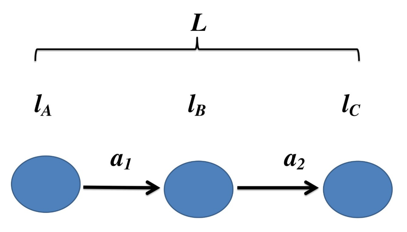

Publisher’s Note: MDPI stays neutral with regard to jurisdictional claims in published maps and institutional affiliations. |
© 2021 by the author. Licensee MDPI, Basel, Switzerland. This article is an open access article distributed under the terms and conditions of the Creative Commons Attribution (CC BY) license (https://creativecommons.org/licenses/by/4.0/).