Article

Accurate Transmission-Less Attenuation Correction Method for Amyloid-β Brain PET Using Deep Neural Network

1
Department of Biomedical Engineering, Gachon University, Incheon 13120, Korea
2
Department of Biomedical Sciences, Seoul National University College of Medicine, Seoul 03080, Korea
3
Department of Nuclear Medicine, Seoul National University Hospital, Seoul 03080, Korea
4
Department of Electronic Engineering, Pai Chai University, Daejeon 35345, Korea
*
Author to whom correspondence should be addressed.
Electronics 2021, 10(15), 1836; https://doi.org/10.3390/electronics10151836
Submission received: 3 May 2021 / Revised: 10 July 2021 / Accepted: 23 July 2021 / Published: 30 July 2021
(This article belongs to the Special Issue Machine Learning for Medical Imaging Processing)

Abstract

:
The lack of physically measured attenuation maps (μ-maps) for attenuation and scatter correction is an important technical challenge in brain-dedicated stand-alone positron emission tomography (PET) scanners. The accuracy of the calculated attenuation correction is limited by the nonuniformity of tissue composition due to pathologic conditions and the complex structure of facial bones. The aim of this study is to develop an accurate transmission-less attenuation correction method for amyloid-β (Aβ) brain PET studies. We investigated the validity of a deep convolutional neural network trained to produce a CT-derived μ-map (μ-CT) from simultaneously reconstructed activity and attenuation maps using the MLAA (maximum likelihood reconstruction of activity and attenuation) algorithm for Aβ brain PET. The performance of three different structures of U-net models (2D, 2.5D, and 3D) were compared. The U-net models generated less noisy and more uniform μ-maps than MLAA μ-maps. Among the three different U-net models, the patch-based 3D U-net model reduced noise and cross-talk artifacts more effectively. The Dice similarity coefficients between the μ-map generated using 3D U-net and μ-CT in bone and air segments were 0.83 and 0.67. All three U-net models showed better voxel-wise correlation of the μ-maps compared to MLAA. The patch-based 3D U-net model was the best. While the uptake value of MLAA yielded a high percentage error of 20% or more, the uptake value of 3D U-nets yielded the lowest percentage error within 5%. The proposed deep learning approach that requires no transmission data, anatomic image, or atlas/template for PET attenuation correction remarkably enhanced the quantitative accuracy of the simultaneously estimated MLAA μ-maps from Aβ brain PET.

1. Introduction

Among the many different physical and technical factors affecting the image quality and quantitative accuracy of position emission tomography (PET) images, attenuation of annihilation photon pairs due to photoelectric absorption and Compton scattering is the single largest factor [1]. In old PET scanners without the combination with computed tomography (CT) or magnetic resonance imaging (MRI), transmission sources with long-lived radioisotopes, such as 68Ga/68Ge and 137Cs, were used to acquire the transmission and blank scans needed for the attenuation correction (AC) in PET [2,3]. In PET/CT, CT images are converted into the PET attenuation map (μ-map) using piecewise linear relationship relationship between the CT Hounsfield Unit and linear attenuation coefficient for 511 eV photons [4,5]. Although PET quantification errors due to artifacts in CT images and spatiotemporal mismatch between CT and PET still exist [6,7,8,9,10], CT-based AC is regarded as a silver standard in PET AC. PET AC in PET/MRI remains an unsolved technical issue because MR images do not provide direct information to measure high-energy photon attenuation [11,12,13,14]. Therefore, several PET AC strategies that do not require CT images have been proposed. Among them, UTE and ZTE MRI-based and atlas-based methods are used for clinical brain PET/MRI studies [15,16,17,18,19,20]. PET AC in whole-body PET/MRI studies relies mainly on Dixon MRI-based μ-maps with no bone segments, leading to large errors in osseous regions [21,22,23]. Recently, various deep learning-based approaches have been proposed to improve the MRI-based PET AC methods, with great potential for replacing conventional approaches [24,25,26,27,28].
With the aging of the global population, neurodegenerative brain disorders such as Alzheimer’s disease and Parkinson’s disease become more prevalent. Visualizing specific biomarkers using PET scans is the most well-proven in vivo approach in major neurodegenerative brain disorders. Therefore, brain-dedicated standalone PET scanners that can provide more affordable solutions for early diagnosis of brain disorders than the current whole-body PET/CT and PET/MRI scanners are actively developed, demanding accurate transmission-less PET AC methods [29,30,31,32]. Although calculated-AC [33] and atlas-based AC [34,35] can be applied to standalone brain PET scanners, the accuracy of these approaches is limited in patients with large anatomical deviations from the normal population [36,37]. Some deep learning-based transmission-less AC methods are showing promise to overcome the limitations of conventional AC approaches for standalone brain PET [24,38,39,40,41,42,43,44].
However, the previous PET AC studies usually focused on 18F-FDG PET scans. Only few methods have been proposed and assessed for amyloid imaging. Dixon MR-based AC caused biases compared to CT-based AC in quantitative analysis for 11C-Pittsburgh compound B (11C-PiB) and 18F-Florbetapir studies [45]. Recently, a deep learning method applied to the integrated UTE/multi-echo Dixon sequence have been proposed for 11C-PiB and 18F-MK-6240 (tau PET imaging) PET/MRI studies [46]. To the best of our knowledge, there is no PET AC study conducted for 18F-Florbetaben.
The aim of this study is to develop an accurate transmission-less attenuation correction method for amyloid-β (Aβ) brain PET studies. Previously, we reported that deep neural networks can improve simultaneous activity and attenuation reconstruction that does not require any transmission data, such as CT [40,41]. However, this new method was validated only for 18F-FP-CIT brain PET for dopamine transporter density assessment [41] and 18F-FDG whole-body PET for glucose metabolism [40]. In this study, we further investigated the validity of a deep neural network trained with simultaneously reconstructed activity and attenuation maps and ground truth CT-based μ-maps for Aβ brain PET. To achieve better quantitative accuracy of attenuation and activity maps, we compared the performance of three different structures (2D, 2.5D, and 3D) of U-net [47] which had achieved good performance in our previous work for improving the simultaneous activity/attenuation reconstruction and many other works [40,41,48,49,50,51,52,53,54,55].
The following sections cover the method followed for collecting brain PET/CT data of 18F-Florbetaben, an Aβ brain PET tracer used in our institution, and the method of designing, training, and testing the networks. Then, the performance of the networks in μ-map prediction and PET quantification is presented to address the question whether 3D learning will lead to network performance improvement in this task.

2. Materials and Methods

2.1. Dataset

Brain 18F-Florbetaben PET/CT scan data of 100 subjects with suspected Alzheimer’s disease (51 amyloid positive and 49 negative, 45 males and 55 females, age: 74.48 ± 7.14 years) were retrospectively analysed. The PET/CT data were acquired using a Siemens Biograph mCT40 scanner (Siemens Healthcare, Knoxville, TN, USA) having a time resolution of 580 ps. The PET/CT imaging was performed for 10 min in a single PET bed position, 90 min after administering an intravenous injection of 18F-Florbetaben (305.9 MBq on average). The head of each participant was positioned in a head holder attached to the patient bed, and the PET/CT scan was conducted by following the routine clinical protocol for brain studies (topogram, CT, and emission PET scans). All datasets were reconstructed using ordered-subset expectation maximization (OSEM, 3 iterations, 21 subsets, 5 mm Gaussian post-filter) with CT-derived attenuation map (μ-CT) and maximum likelihood reconstruction of activity and attenuation (MLAA, 6 iterations, 21 subsets, 5 mm Gaussian post-filter) with time-of-flight (TOF) information [56,57,58,59]. To mitigate the non-unique global scaling problem in the MLAA, the boundary constraint was applied during the attenuation image estimation in the MLAA. The initial μ-map estimate of the MLAA was a uniform image filled with 1.0. Scatter sinogram was estimated from μ-CT using single scatter simulation. The dimensions and voxel size of the reconstructed PET images were 200 × 200 × 109 and 2.04 mm × 2.04 mm × 2.03 mm, respectively. To obtain μ-CT, the CT images that had the dimensions and voxel size of 512 × 512 × 149 and 0.59 mm × 0.59 mm × 1.5 mm, respectively, were resampled to have the same dimensions and voxel size as the PET images.

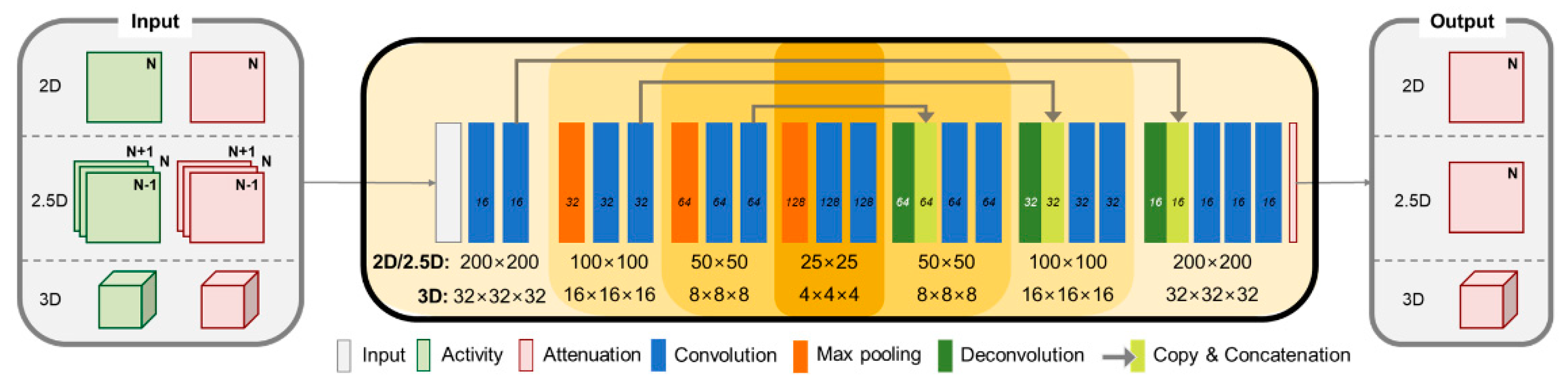
2.2. Network Architecture

As mentioned previously, three different U-net models (2D, 2.5D, and 3D) were designed, trained, and tested. The U-net models were trained to produce μ-maps equivalent to μ-CT once the activity and attenuation maps obtained from the MLAA (λ-MLAA and μ-MLAA) are given to the U-net as input (Figure 1). All the input and output image sizes were 200 × 200 for the 2D U-net models (slice-to-slice translation), which is a straightforward structure. For the 3D U-net models, input voxel patches with a size of 32 × 32 × 32 in head pixels were extracted from λ-MLAA and μ-MLAA, with stride 4. Three-dimensional (3D) U-net is expected to provide more accurate attenuation maps with reduced axial discontinuities using extensive local information from 3D patches. The 2.5D U-net was designed to produce a central slice once three neighboring slices with a size of 200 × 200 were provided to the network (slab-to-slice translation). The 2.5D U-net was a compromise between 2D U-net and 3D U-net employing whole transaxial planes to reduce in-plane discontinuities, as well as providing additional information from neighboring slices. The input image intensity was normalized to a range of 0–1.
The U-net models consisted of convolution layers, rectified linear units (ReLU), 2 × 2 max pooling layers (2 × 2 × 2 in 3D networks), deconvolution layers, and a 1 × 1 (1 × 1 × 1 in 3D networks) convolution layer. In the contracting path, the 3 × 3 convolutions (3 × 3 × 3 in 3D networks) and ReLU function were repeated twice for each layer; further, the image dimension was reduced by half while the number of features was doubled by applying 2 × 2 max pooling (2 × 2 × 2 in 3D networks) with a stride of 2. In the expanding path, the image dimension was doubled, and the number of features was reduced by half by applying 2 × 2 up-convolution (2 × 2 × 2 in 3D networks) that used the nearest-neighbour interpolation. The concatenation operator was applied by the skip connections of the cropped feature map before max pooling in the contracting path to the expanding path. We implemented the networks using the TensorFlow library.

2.3. Training and Validation

The cost function was the L1-norm between the U-net output (μ-CNN) and μ-CT. The cost function was minimized using the adaptive moment estimation method (Adam optimization). The network weights were initialized using the Xavier method, which assigns random weights considering the number of inputs and outputs [60]. The batch size was 30 in the 2D and 2.5D networks, and it was 100 in the 3D network. The number of epochs was 50 in the 2D and 2.5D networks, it was and 20 in the 3D network. The learning rate was initially 0.001 for all the networks, and it was reduced for each epoch by 0.5, 0.5, and 0.8 times in the 2D, 2.5D, and 3D networks, respectively.
The training data were shuffled before each epoch to create randomization in the batch training. While using the Ryzen 1700X CPU with a GTX 1080 GPU, each epoch took approximately 12, 23, and 180 min for the 2D, 2.5D, and 3D networks, respectively.
We performed five-fold cross-validation to evaluate the performance of the networks. Accordingly, the 100 datasets were divided into 5 groups of 20 datasets in random order (20 in each group). In each cross-validation study, 3 groups (total: 60 datasets) were used for training the networks, 1 group (20 datasets) was used for training validation, and the remaining group (20 datasets) was used for evaluation. Supplementary Figure S1 shows the validation error learning curve for 2D, 2.5D, and 3D networks along the training epochs.

2.4. Image Analysis

The maps μ-MLAA and μ-CNNs were compared with μ-CT, the ground truth. The similarity of the μ-maps was evaluated using the Dice similarity coefficient, voxel-wise correlation, normalized root mean square error (NRMSE), and peak signal-to-noise ratio (PSNR) [41,52]. The Dice similarity coefficient was calculated for the air and bone segments. The voxels with μ-values greater than 0.1134 (=300 Hounsfield units) were regarded as bone segment; those with μ-values less than 0.0475 (=−500 Hounsfield units) were regarded as air segment [41]. In addition, the voxels with μ-values between the above limits were regarded as soft tissue. The Dice similarity coefficient was calculated using the following equation
D = 2 × N μ -C T     μ - P E T N μ - C T + N μ - P E T
where Nµ-CT and Nµ-PET are the number of bone (or air) voxels in the μ-maps derived from CT (μ-CT) and PET (μ-MLAA or μ-CNNs) data, respectively. N(µ-CTµ-PET) indicates the number of overlapped voxels between the μ-maps from CT and PET.
The NRMSE enables comparison between the datasets of models with different scales, and the PSNR is a quantitative measure of the differences between two images.
P S N R = 10 × log 10 M a x μ - C T 2 M S E
N R M S E = M S E M a x μ - C T M i n μ - C T
M S E = 1 m n i = 0 m 1 j = 0 n 1 I i , j     K i , j 2
where Max and Min are the maximum and minimum intensities, respectively, of the reference image, μ-CT. MSE is the average value of the squared error between μ-CT and μ-CNN or μ-CNNs, and m and n are the width and height in pixels, respectively, of the image.
The PSNR measurement was also performed on the activity images reconstructed using the different μ-maps and the OSEM algorithm. Regional analysis was also performed in the same manner as in our previous study with 18F-FP-CIT brain PET [41]. The ground-truth PET activity images, corrected for attenuation using μ-CT, were spatially normalized using statistical parametric mapping software (http://www.fil.ion.ucl.ac.uk/spm, accessed on: 1 August 2019), and the same transformation parameters were applied to the images corrected using μ-MLAA and μ-CNNs. The standard uptake value (SUV) and SUV ratio relative to the reference region (SUVr) were measured using the automatic regions of interest (ROIs) predefined by the statistical probabilistic anatomic maps [61,62].

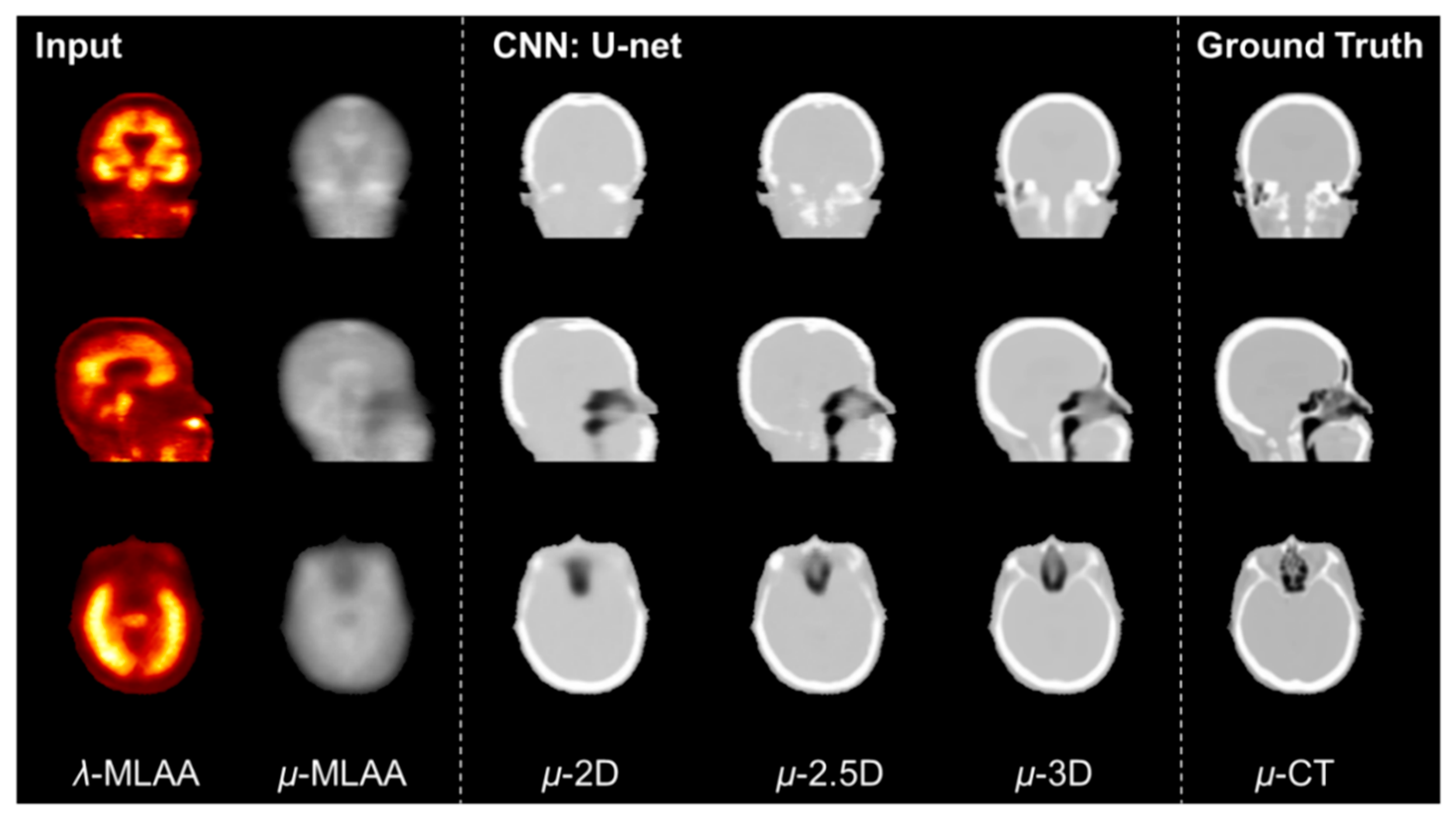
2.5. Comparison between 2D, 2.5D, and 3D U-Net

Training the 2D network is fast and requires less memory compared to training the 3D network. However, stacking 2D network outputs to generate 3D attenuation maps leads to discontinuities in the axial dimension. On the other hand, training the 3D network is computationally expensive and requires much more memory. As training a 3D network using whole PET images is generally difficult, training with 3D patches extracted from whole PET images is usually employed. However, 3D patch-based inference would also lead to discontinuities at the borders of patches. The 2.5D networks have been proposed as a compromise between 2D and 3D, using multi-slice inputs. The 2D and 3D networks are evaluated in the previous studies using different tracers using 18F-FP-CIT and 18F-FDG, respectively [40,41], but there are no direct comparison using a same tracer among 2D, 2.5D, and 3D networks. In this study, we compared these architectures with evaluation measures stated above.

2.6. Comparison between Single-Image Input and Multi-Input

As noise patterns and cross-talk artifacts in λ-MLAA and μ-MLAA are highly correlated, our networks were designed to exploit some useful features from combination of λ-MLAA and μ-MLAA to solve the problems when generating attenuation maps. By doing so, we expect that better performance could be achieved compared to when employing only λ-MLAA or μ-MLAA as an input. To explore the relative importance of λ-MLAA and μ-MLAA input, a 3D network was additionally trained with each of two separately and tested.

3. Results

The μ-MLAA appeared very different from μ-CT, mainly owing to severe cross-talk artefacts between the activity and attenuation maps generated by MLAA. On the other hand, the U-net models generated less noisy and more uniform μ-maps (Figure 2). The μ-maps estimated using the original MLAA were considerably underestimated, which was mitigated by applying the deep neural networks. The performance of patch-based 3D learning was superior to those of 2D slice-to-slice and 2.5D slab-to-slice translations (Figure 2, Figure 3 and Figure 4, and Table 1). The 2.5D U-net models did not yield performance improvement in comparison with 2D.
Figure 4 shows the plots of the NRMSE between μ-maps along the axial slice location in a representative patient, as shown in Figure 2 and Figure 3. As shown in this figure, the error relative to μ-CT (ground truth μ-map) was dramatically reduced by applying the deep neural networks to the MLAA output images. In this case, the NRMSE decreased as the dimensions of the model increased from 2D to 3D. However, the incremental gain from 2D to 2.5D was not as high as that from 2.5D to 3D. The 3D patch-based learning was also useful in eliminating the discontinuity of pixel values in the axial direction, as shown in the output of 2D networks (Figure 2). Figure 4 also shows that the NRMSE between μ-CNNs and μ-CT is larger in the facial bone areas (smaller-numbered slices in Figure 4) such as the nasal cavity than in the cranial regions.
The deep neural networks resulted in a significant improvement from μ-MLAA to μ-CNNs in the measurement of Dice similarity coefficients relative to μ-CNN (Table 1). The inaccuracy of μ-MLAA disabled proper segmentation of bone and air regions based on the μ-values. The Dice similarity coefficients between μ-MLAA and μ-CT in bone and air segments obtained here with 18F-Florbetaben PET data (0.073 and 0.055) were smaller than those obtained in our previous study conducted with 18F-FP-CIT PET (0.374 and 0.317) [41]. In both the bone and air segments, the mean Dice similarity coefficients increased, and their standard deviations decreased by applying the deep neural networks. The 3D patch-based learning yielded higher similarity in the bone and air segmentation to the ground truth than 2D or 2.5 learnings. Although the 2D U-net yielded a lower Dice similarity coefficient (0.718 and 0.400 in bone and air, respectively) than the previous study 18F-FP-CIT PET, in which the 2D U-net was also applied (0.787 and 0.575), the 3D U-net achieved better results (0.826 and 0.674).
The voxel-wise correlation of μ-maps are summarized in Table 2, showing the improved accuracy of the μ-map by CNN. All three U-net models showed better voxel-wise correlation of the μ-maps compared to MLAA. The patch-based 3D U-net model was the best.
The PSNR evaluation summarized in Table 3 also shows improved μ-map generation and PET quantification achieved by applying the 3D patch-based learning. There were at least 18 dB PSNR improvements in the μ-map and PET activity data, respectively, by applying DL to the MLAA outputs, and the improvement was the largest with 3D U-nets. Figure 5 shows the activity images corrected for attenuation using different μ-maps and reconstructed using the OSEM algorithm, and the SUV error map was relative to the ground truth (corrected image using μ-CT).
ROI analysis was conducted in four regions (putamen, caudate head, cerebellum, and occipital cortex) using activity maps that were attenuation-corrected using the proposed μ-maps. In addition, percentage errors of SUV and SUVr were calculated (Figure 6). While the uptake value of MLAA yielded a high percentage error of 20% or more, the uptake value of 3D U-nets yielded the lowest percentage error within 5%. Furthermore, the standard deviation of MLAA was larger than that of the CNN outcomes. In both SUV and SUVr quantification, the 3D U-nets showed a smaller bias and dispersion than the 2D or 2.5D U-nets.
The results of network training using only λ-MLAA or μ-MLAA are shown in Figure 7. The errors in attenuation map generation were much smaller than original MLAA. However, the combined input (λ-MLAA and μ-MLAA) yielded the smallest error, as shown Figure 7. The amount of error in the networks trained using only λ-MLAA and μ-MLAA was almost identical.

4. Discussion

In this study, we compared the performance of three different CNN schemes based on the U-net structure to predict μ-CT from the outcomes of MLAA simultaneous activity and attenuation reconstruction for 18F-Florbetaben Aβ PET. As shown in the results, the 3D patch-based learning used in our previous work for whole-body 18F-FDG PET [40] outperformed the 2D slice-to-slice translation strategy that was used in the 18F-FP-CIT brain PET study [23]. Although the addition of neighboring slices in the input (2.5D slab-to-slice translation) improved the μ-map prediction performance, the improvement was not remarkably high. The general performance of the original MLAA in the prediction of μ-map for 18F-Florbetaben was inferior to that of 18F-FP-CIT [41]. However, the 3D patch-based learning could overcome this limitation of MLAA and enabled accurate PET quantification. The improved performance using 3D patch-based learning compared to using 2.5D slab-to-slice translation is much higher than between 2.5D slab-to-slice translation and 2D slice-to-slice translation (Figure 4 and Table 1, Table 2 and Table 3). Extensive local information from 3D patch would allow CNN to better extract the features of the attenuation map, whereas only three slices from the 2.5D slab would not be enough to make significant improvement in the CNN performance.
As shown in Figure 4, the error in predicting μ-CT was higher in the facial bone regions than in the cranial bone regions. This implies that the deep learning-based approach used in this study was not sufficiently good for reconstructing the fine anatomical details in the facial bone regions. However, this inferior result mainly appears to originate from the poor anatomical information provided by the MLAA reconstruction. Improved MLAA performance in more advanced PET systems with better timing resolution will be useful in overcoming the limitations of the proposed method [63,64,65]. Another useful approach that we should try in future studies is the modification of the loss function to obtain better-trained networks. Recently, Shi et al. showed improvement in the present method for whole-body 18F-FDG PET studies by adding an additional loss function in the projection space (integration of attenuation coefficient along the line of response) to the image fidelity loss [43]. This modification would be highly relevant, because the PET AC is performed in the projection space and not in the reconstructed image space. Further investigations are required on the advanced loss functions for the Aβ brain PET data.
As shown in Figure 7, training with combined input (λ-MLAA and μ-MLAA) achieved better convergence and yielded the smaller errors compared to training with only λ-MLAA or μ-MLAA. This implies that both λ-MLAA and μ-MLAA are advantageous for network to suppress noise levels and reduce cross-talk artifacts in attenuation map generation. In addition, the accuracy of training using only λ-MLAA and μ-MLAA was almost identical. This indicates that the importance of λ-MLAA and μ-MLAA to the networks is almost identical. Perhaps, the superior performance of the proposed method would be mainly attributed to the utilization of combined inputs for generating enhanced attenuation maps, while conventional approaches focused on only manipulating μ-MLAA by applying a background prior and using constrained Gaussian mixture models [58,66].
There are a growing number of PET AC studies that have reported AC performance improvement by introducing generative adversarial networks (GAN) [38,39,67]. We have also attempted to apply a conditional GAN method that was effective in our previous studies on PET to MRI transformation and Aβ PET template generation [68,69] to the present task. However, we could not achieve significant performance improvement in the μ-map prediction.
Another active transmission-less approach for PET AC is the deep learning-based conversion of non-attenuation-corrected PET images to the μ-map or attenuation-corrected PET image [19]. Initial studies on this approach have also shown promising results in 18F-FDG brain and whole-body PET studies. However, studies on tracers other than 18F-FDG have rarely been conducted.
When compared to the MRI-based AC methods applied to the amyloid and tau PET dataset [47], our 3D patch-based learning with no MRI input shows comparable results with CNN employing Dixon sequence and is slightly inferior to CNN employing integrated UTE/multi-echo Dixon sequence (Dice coefficient: ours = 0.83, CNN-Dixon = 0.84, CNN-integrated UTE/multi-echo Dixon = 0.87). However, this comparison only serves as a reference because the radiotracer and enrolled patients are different.
Our method has been validated using various tracers including 18F-FP-CIT, 18F-FDG, 68Ga-DOTATOC [40,41,70], and 18F-Florbetaben (this study). A limitation of this study is that we currently need to re-train the network from the scratch for applying this method to new radiopharmaceutical. Thus, a large number of scans is required for each radiopharmaceutical. To overcome this limitation, transfer learning that reuses a model developed for “old” tracers as the starting point for a model on “new” tracers should be considered as future works.
In addition, this attenuation map generation might be useful for other diagnosis supporting tasks including classification, segmentation, prediction, and detection [71,72,73,74].

5. Conclusions

We have proposed an attenuation correction method using MLAA with deep learning. The proposed deep learning approach that requires no transmission data, anatomic image, or atlas/template for PET attenuation correction remarkably enhanced the quantitative accuracy of the simultaneously estimated MLAA μ-maps from Aβ brain PET. The benefit of using 2.5D slab-to-slice translation was not significant compared to using 2D slice-to-slice translation. The approach using 3D patch outperformed the others. The combined input of λ-MLAA and μ-MLAA could reduce the error of generated attenuation maps compared to single input of λ-MLAA or μ-MLAA. Both λ-MLAA and μ-MLAA have almost equal contributions for accuracy of the proposed method. Further study might be needed to apply the proposed method on “new” tracers, utilizing previous trained networks. This attenuation map generation would be applied to other diagnosis supporting tasks as well as the attenuation correction task.

Supplementary Materials

Supplementary Materials are available online at https://www.mdpi.com/article/10.3390/electronics10151836/s1.

Author Contributions

Conceptualization, B.-H.C., D.H., and J.-S.L.; data curation, D.H.; methodology and investigation, B.-H.C., and D.H.; formal analysis, B.-H.C., and S.S.; writing—original draft, B.-H.C., D.H.; writing—review and editing, S.-K.K., K.-Y.K., H.C., S.S., and J.-S.L.; supervision, H.C., and J.-S.L.; funding acquisition, J.-S.L. All authors have read and agreed to the published version of the manuscript.

Funding

This work was supported by the grants issued by the National Research Foundation of Korea (NRF) and funded by the Korean Ministry of Science and ICT (Grant No. NRF-2016R1A2B3014645); the Korea Medical Device Development Fund grant funded by the Korea government (Project no. 202011A06-03). The funding source had no involvement in the study design, collection, analysis, or interpretation.

Institutional Review Board Statement

The study was conducted according to the guidelines of the Declaration of Helsinki, and approved by the Institutional Review Board) of Seoul National University Hospital (protocol code: 1711-140-903, approved: 11 December 2017).

Informed Consent Statement

Patient consent was waived due to retrospective nature of the study and the analysis used anonymous clinical data.

Data Availability Statement

The data presented in this study are available on request from the corresponding author. The data are not publicly available due to ethical issues.

Conflicts of Interest

No other potential conflict of interest relevant to this article was reported.

Abbreviations

PETPositron emission tomography
CTComputed tomography
MRIMagnetic resonance imaging
ACAttenuation correction
μ-mapAttenuation map
Amyloid-β
OSEMOrdered-subset expectation maximisation
μ-CTCT-derived attenuation map
MLAAMaximum likelihood reconstruction of activity and attenuation
λ-MLAAActivity maps obtained from the MLAA
μ-MLAAAttenuation maps obtained from the MLAA
ReLURectified linear units
μ-CNNU-net output
NRMSENormalized root mean square error
PSNRPeak signal-to-noise ratio
SUVStandard uptake value
SUVrSUV ratio relative to the reference region
ROIRegion of interest
GANGenerative adversarial network

References

  1. Cherry, S.R.; Dahlbom, M.; Phelps, M.E. PET: Physics, Instrumentation, and Scanners. In PET; Springer: New York, NY, USA, 2004; pp. 1–124. [Google Scholar]
  2. Bailey, D.L. Transmission scanning in emission tomography. Eur. J. Nucl. Med. Mol. Imaging 1998, 25, 774–787. [Google Scholar] [CrossRef]
  3. Zaidi, H.; Hasegawa, B. Determination of the attenuation map in emission tomography. J. Nucl. Med. 2003, 44, 291–315. [Google Scholar]
  4. Kinahan, P.; Hasegawa, B.H.; Beyer, T. X-ray-based attenuation correction for positron emission tomography/computed tomography scanners. Semin. Nucl. Med. 2003, 33, 166–179. [Google Scholar] [CrossRef]
  5. Townsend, D.W. Dual-Modality Imaging: Combining Anatomy and Function. J. Nucl. Med. 2008, 49, 938–955. [Google Scholar] [CrossRef] [PubMed] [Green Version]
  6. Choi, Y.Y.; Lee, J.S.; Yang, S.-O. Musculoskeletal Lesions: Nuclear Medicine Imaging Pitfalls. In Pitfalls in Musculoskeletal Radiology; Springer Science and Business Media LLC: New York, NY, USA, 2017; pp. 951–976. [Google Scholar]
  7. Goerres, G.W.; Ziegler, S.I.; Burger, C.; Berthold, T.; Von Schulthess, G.K.; Buck, A. Artifacts at PET and PET/CT Caused by Metallic Hip Prosthetic Material. Radiology 2003, 226, 577–584. [Google Scholar] [CrossRef] [PubMed]
  8. Kamel, E.M.; Burger, C.; Buck, A.; Von Schulthess, G.K.; Goerres, G.W. Impact of metallic dental implants on CT-based attenuation correction in a combined PET/CT scanner. Eur. Radiol. 2003, 13, 724–728. [Google Scholar] [CrossRef]
  9. Lodge, M.A.; Mhlanga, J.C.; Cho, S.Y.; Wahl, R.L. Effect of Patient Arm Motion in Whole-Body PET/CT. J. Nucl. Med. 2011, 52, 1891–1897. [Google Scholar] [CrossRef] [PubMed] [Green Version]
  10. Mawlawi, O.; Erasmus, J.J.; Pan, T.; Cody, D.D.; Campbell, R.; Lonn, A.H.; Kohlmyer, S.; Macapinlac, H.A.; Podoloff, D.A. Truncation Artifact on PET/CT: Impact on Measurements of Activity Concentration and Assessment of a Correction Algorithm. Am. J. Roentgenol. 2006, 186, 1458–1467. [Google Scholar] [CrossRef]
  11. Keereman, V.; Mollet, P.; Berker, Y.; Schulz, V.; Vandenberghe, S. Challenges and current methods for attenuation correction in PET/MR. Magma Magn. Reson. Mater. Phys. Biol. Med. 2012, 26, 81–98. [Google Scholar] [CrossRef]
  12. Vandenberghe, S.; Marsden, P.K. PET-MRI: A review of challenges and solutions in the development of integrated multimodality imaging. Phys. Med. Biol. 2015, 60, R115–R154. [Google Scholar] [CrossRef] [PubMed]
  13. Yoo, H.J.; Lee, J.S.; Lee, J.M. Integrated whole body MR/PET: Where are we? Korean J. Radiol. 2015, 16, 32–49. [Google Scholar] [CrossRef] [PubMed] [Green Version]
  14. Chen, Y.; An, H. Attenuation Correction of PET/MR Imaging. Magn. Reson. Imaging Clin. N. Am. 2017, 25, 245–255. [Google Scholar] [CrossRef] [Green Version]
  15. An, H.J.; Seo, S.; Kang, H.; Choi, H.; Cheon, G.J.; Kim, H.-J.; Lee, D.S.; Song, I.-C.; Kim, Y.K.; Lee, J.S. MRI-Based Attenuation Correction for PET/MRI Using Multiphase Level-Set Method. J. Nucl. Med. 2016, 57, 587–593. [Google Scholar] [CrossRef] [Green Version]
  16. Catana, C.; Van Der Kouwe, A.; Benner, T.; Michel, C.J.; Hamm, M.; Fenchel, M.; Fischl, B.; Rosen, B.; Schmand, M.; Sorensen, A.G. Toward Implementing an MRI-Based PET Attenuation-Correction Method for Neurologic Studies on the MR-PET Brain Prototype. J. Nucl. Med. 2010, 51, 1431–1438. [Google Scholar] [CrossRef] [Green Version]
  17. Delso, G.; Wiesinger, F.; Sacolick, L.I.; Kaushik, S.S.; Shanbhag, D.D.; Hüllner, M.; Veit-Haibach, P. Clinical Evaluation of Zero-Echo-Time MR Imaging for the Segmentation of the Skull. J. Nucl. Med. 2015, 56, 417–422. [Google Scholar] [CrossRef] [PubMed] [Green Version]
  18. Keereman, V.; Fierens, Y.; Broux, T.; De Deene, Y.; Lonneux, M.; Vandenberghe, S. MRI-Based Attenuation Correction for PET/MRI Using Ultrashort Echo Time Sequences. J. Nucl. Med. 2010, 51, 812–818. [Google Scholar] [CrossRef] [PubMed] [Green Version]
  19. Montandon, M.-L.; Zaidi, H. Atlas-guided non-uniform attenuation correction in cerebral 3D PET imaging. NeuroImage 2005, 25, 278–286. [Google Scholar] [CrossRef]
  20. Yang, J.; Wiesinger, F.; Kaushik, S.; Shanbhag, D.; Hope, T.A.; Larson, P.E.Z.; Seo, Y. Evaluation of Sinus/Edge-Corrected Zero-Echo-Time-Based Attenuation Correction in Brain PET/MRI. J. Nucl. Med. 2017, 58, 1873–1879. [Google Scholar] [CrossRef] [Green Version]
  21. Hofmann, M.; Bezrukov, I.; Mantlik, F.; Aschoff, P.; Steinke, F.; Beyer, T.; Pichler, B.J.; Schölkopf, B. MRI-Based Attenuation Correction for Whole-Body PET/MRI: Quantitative Evaluation of Segmentation- and Atlas-Based Methods. J. Nucl. Med. 2011, 52, 1392–1399. [Google Scholar] [CrossRef] [Green Version]
  22. Kim, J.H.; Lee, J.S.; Song, I.-C.; Lee, D.S. Comparison of Segmentation-Based Attenuation Correction Methods for PET/MRI: Evaluation of Bone and Liver Standardized Uptake Value with Oncologic PET/CT Data. J. Nucl. Med. 2012, 53, 1878–1882. [Google Scholar] [CrossRef] [Green Version]
  23. Martinez-Möller, A.; Souvatzoglou, M.; Delso, G.; Bundschuh, R.A.; Chefd’Hotel, C.; Ziegler, S.I.; Navab, N.; Schwaiger, M.; Nekolla, S.G. Tissue Classification as a Potential Approach for Attenuation Correction in Whole-Body PET/MRI: Evaluation with PET/CT Data. J. Nucl. Med. 2009, 50, 520–526. [Google Scholar] [CrossRef] [PubMed] [Green Version]
  24. Lee, J.S. A Review of Deep-Learning-Based Approaches for Attenuation Correction in Positron Emission Tomography. IEEE Trans. Radiat. Plasma Med. Sci. 2021, 5, 160–184. [Google Scholar] [CrossRef]
  25. Jang, H.; Liu, F.; Zhao, G.; Bradshaw, T.; McMillan, A.B. Technical Note: Deep learning based MRAC using rapid ultrashort echo time imaging. Med. Phys. 2018, 45, 3697–3704. [Google Scholar] [CrossRef] [PubMed]
  26. Ladefoged, C.N.; Marner, L.; Hindsholm, A.; Law, I.; Højgaard, L.; Andersen, F.L. Deep Learning Based Attenuation Correction of PET/MRI in Pediatric Brain Tumor Patients: Evaluation in a Clinical Setting. Front. Neurosci. 2019, 12, 1005. [Google Scholar] [CrossRef] [PubMed]
  27. Leynes, A.P.; Yang, J.; Wiesinger, F.; Kaushik, S.S.; Shanbhag, D.D.; Seo, Y.; Hope, T.A.; Larson, P.E.Z. Zero-Echo-Time and Dixon Deep Pseudo-CT (ZeDD CT): Direct Generation of Pseudo-CT Images for Pelvic PET/MRI Attenuation Correction Using Deep Convolutional Neural Networks with Multiparametric MRI. J. Nucl. Med. 2017, 59, 852–858. [Google Scholar] [CrossRef] [PubMed]
  28. Torrado-Carvajal, A.; Vera-Olmos, J.; Izquierdo-Garcia, D.; Catalano, O.A.; Morales, M.A.; Margolin, J.; Soricelli, A.; Salvatore, M.; Malpica, N.; Catana, C. Dixon-VIBE Deep Learning (DIVIDE) Pseudo-CT Synthesis for Pelvis PET/MR Attenuation Correction. J. Nucl. Med. 2019, 60, 429–435. [Google Scholar] [CrossRef] [Green Version]
  29. Ahmed, A.M.; Tashima, H.; Yoshida, E.; Nishikido, F.; Yamaya, T. Simulation study comparing the helmet-chin PET with a cylindrical PET of the same number of detectors. Phys. Med. Biol. 2017, 62, 4541–4550. [Google Scholar] [CrossRef]
  30. Gonzalez, A.J.; Sanchez, F.; Benlloch, J.M. Organ-Dedicated Molecular Imaging Systems. IEEE Trans. Radiat. Plasma Med. Sci. 2018, 2, 388–403. [Google Scholar] [CrossRef]
  31. Majewski, S.R.; Proffitt, J.; Brefczynski-Lewis, J.; Stolin, A.; Weisenberger, A.; Xi, W.; Wojcik, R. HelmetPET: A silicon photomultiplier based wearable brain imager. In Proceedings of the 2011 IEEE Nuclear Science Symposium Conference Record, Valencia, Spain, 23–29 October 2012; pp. 4030–4034. [Google Scholar] [CrossRef]
  32. Yamamoto, S.; Honda, M.; Oohashi, T.; Shimizu, K.; Senda, M. Development of a Brain PET System, PET-Hat: A Wearable PET System for Brain Research. IEEE Trans. Nucl. Sci. 2011, 58, 668–673. [Google Scholar] [CrossRef]
  33. Bergström, M.; Litton, J.; Eriksson, L.; Bohm, C.; Blomqvist, G. Determination of Object Contour from Projections for Attenuation Correction in Cranial Positron Emission Tomography. J. Comput. Assist. Tomogr. 1982, 6, 365–372. [Google Scholar] [CrossRef]
  34. Kops, E.R.; Herzog, H. Alternative methods for attenuation correction for PET images in MR-PET scanners. In Proceedings of the 2007 IEEE Nuclear Science Symposium Conference Record, Honolulu, HI, USA, 26 October–3 November 2007; Volume 6, pp. 4327–4330. [Google Scholar] [CrossRef]
  35. Sekine, T.; Buck, A.; Delso, G.; ter Voert, E.; Huellner, M.; Veit-Haibach, P.; Warnock, G. Evaluation of Atlas-Based Attenuation Correction for Integrated PET/MR in Human Brain: Application of a Head Atlas and Comparison to True CT-Based Attenuation Correction. J. Nucl. Med. 2016, 57, 215–220. [Google Scholar] [CrossRef] [Green Version]
  36. Hooper, P.K.; Meikle, S.; Eberl, S.; Fulham, M.J. Validation of postinjection transmission measurements for attenuation correction in neurological FDG-PET studies. J. Nucl. Med. 1996, 37, 128–136. [Google Scholar]
  37. Kaneko, K.; Kuwabara, Y.; Sasaki, M.; Koga, H.; Abe, K.; Baba, S.; Hayashi, K.; Honda, H. Validation of quantitative accuracy of the post-injection transmission-based and transmissionless attenuation correction techniques in neurological FDG-PET. Nucl. Med. Commun. 2004, 25, 1095–1102. [Google Scholar] [CrossRef]
  38. Dong, X.; Lei, Y.; Wang, T.; Higgins, K.; Liu, T.; Curran, W.J.; Mao, H.; Nye, J.A.; Yang, X. Deep learning-based attenuation correction in the absence of structural information for whole-body positron emission tomography imaging. Phys. Med. Biol. 2020, 65, 055011. [Google Scholar] [CrossRef] [PubMed]
  39. Dong, X.; Wang, T.; Lei, Y.; Higgins, K.; Liu, T.; Curran, W.J.; Mao, H.; A Nye, J.; Yang, X. Synthetic CT generation from non-attenuation corrected PET images for whole-body PET imaging. Phys. Med. Biol. 2019, 64, 215016. [Google Scholar] [CrossRef] [PubMed]
  40. Hwang, D.; Kang, S.K.; Kim, K.Y.; Seo, S.; Paeng, J.C.; Lee, D.S.; Lee, J.S. Generation of PET Attenuation Map for Whole-Body Time-of-Flight 18F-FDG PET/MRI Using a Deep Neural Network Trained with Simultaneously Reconstructed Activity and Attenuation Maps. J. Nucl. Med. 2019, 60, 1183–1189. [Google Scholar] [CrossRef] [PubMed] [Green Version]
  41. Hwang, D.; Kim, K.Y.; Kang, S.K.; Seo, S.; Paeng, J.C.; Lee, D.S.; Lee, J.S. Improving the Accuracy of Simultaneously Reconstructed Activity and Attenuation Maps Using Deep Learning. J. Nucl. Med. 2018, 59, 1624–1629. [Google Scholar] [CrossRef] [PubMed]
  42. Liu, F.; Jang, H.; Kijowski, R.; Zhao, G.; Bradshaw, T.; McMillan, A.B. A deep learning approach for 18F-FDG PET attenuation correction. EJNMMI Phys. 2018, 5, 24. [Google Scholar] [CrossRef] [PubMed]
  43. Shi, L.; Onofrey, J.A.; Revilla, E.M.; Toyonaga, T.; Menard, D.; Ankrah, J.; Carson, R.E.; Liu, C.; Lu, Y. A Novel Loss Function Incorporating Imaging Acquisition Physics for PET Attenuation Map Generation Using Deep Learning. In Transactions on Petri Nets and Other Models of Concurrency XV; Springer Science and Business Media LLC: New York, NY, USA, 2019; pp. 723–731. [Google Scholar]
  44. Shiri, I.; Ghafarian, P.; Geramifar, P.; Leung, K.H.-Y.; Oghli, M.G.; Oveisi, M.; Rahmim, A.; Ay, M.R. Direct attenuation correction of brain PET images using only emission data via a deep convolutional encoder-decoder (Deep-DAC). Eur. Radiol. 2019, 29, 6867–6879. [Google Scholar] [CrossRef]
  45. Su, Y.; Rubin, B.B.; McConathy, J.; Laforest, R.; Qi, J.; Sharma, A.; Priatna, A.; Benzinger, T.L. Impact of MR-Based Attenuation Correction on Neurologic PET Studies. J. Nucl. Med. 2016, 57, 913–917. [Google Scholar] [CrossRef] [PubMed] [Green Version]
  46. Gong, K.; Han, P.K.; Johnson, K.A.; El Fakhri, G.; Ma, C.; Li, Q. Attenuation correction using deep Learning and integrated UTE/multi-echo Dixon sequence: Evaluation in amyloid and tau PET imaging. Eur. J. Nucl. Med. Mol. Imaging 2021, 48, 1351–1361. [Google Scholar] [CrossRef] [PubMed]
  47. Ronneberger, O.; Fischer, P.; Brox, T. U-net: Convolutional networks for biomedical image segmentation. In Proceedings of the International Conference on Medical Image Computing and Computer-Assisted Intervention, Munich, Germany, 5–9 October 2015; Springer: Cham, Switzerland, 2015; pp. 234–241. [Google Scholar]
  48. Han, Y.; Ye, J.C. Framing U-Net via Deep Convolutional Framelets: Application to Sparse-View CT. IEEE Trans. Med Imaging 2018, 37, 1418–1429. [Google Scholar] [CrossRef] [PubMed] [Green Version]
  49. Hegazy, M.A.A.; Cho, M.H.; Cho, M.H.; Lee, S.Y. U-net based metal segmentation on projection domain for metal artifact reduction in dental CT. Biomed. Eng. Lett. 2019, 9, 375–385. [Google Scholar] [CrossRef]
  50. Lee, M.S.; Hwang, D.; Kim, J.H.; Lee, J.S. Deep-dose: A voxel dose estimation method using deep convolutional neural network for personalized internal dosimetry. Sci. Rep. 2019, 9, 1–9. [Google Scholar] [CrossRef] [Green Version]
  51. Park, J.; Bae, S.; Seo, S.; Park, S.; Bang, J.-I.; Han, J.H.; Lee, W.W.; Lee, J.S. Measurement of Glomerular Filtration Rate using Quantitative SPECT/CT and Deep-learning-based Kidney Segmentation. Sci. Rep. 2019, 9, 1–8. [Google Scholar] [CrossRef] [PubMed] [Green Version]
  52. Park, J.; Hwang, D.; Kim, K.Y.; Kang, S.K.; Kim, Y.K.; Lee, J.S. Computed tomography super-resolution using deep convolutional neural network. Phys. Med. Biol. 2018, 63, 145011. [Google Scholar] [CrossRef]
  53. Sevastopolsky, A. Optic disc and cup segmentation methods for glaucoma detection with modification of U-Net convolutional neural network. Pattern Recognit. Image Anal. 2017, 27, 618–624. [Google Scholar] [CrossRef] [Green Version]
  54. Yie, S.Y.; Kang, S.K.; Hwang, D.; Lee, J.S. Self-supervised PET Denoising. Nucl. Med. Mol. Imaging 2020, 54, 299–304. [Google Scholar] [CrossRef]
  55. Kang, S.K.; Shin, S.A.; Seo, S.; Byun, M.S.; Lee, D.Y.; Kim, Y.K.; Lee, D.S.; Lee, J.S. Deep learning-Based 3D inpainting of brain MR images. Sci. Rep. 2021, 11, 1–11. [Google Scholar] [CrossRef]
  56. Aasheim, L.B.; Karlberg, A.; Goa, P.E.; Håberg, A.; Sørhaug, S.; Fagerli, U.-M.; Eikenes, L. PET/MR brain imaging: Evaluation of clinical UTE-based attenuation correction. Eur. J. Nucl. Med. Mol. Imaging 2015, 42, 1439–1446. [Google Scholar] [CrossRef] [PubMed]
  57. Defrise, M.; Rezaei, A.; Nuyts, J. Time-of-flight PET data determine the attenuation sinogram up to a constant. Phys. Med. Biol. 2012, 57, 885–899. [Google Scholar] [CrossRef]
  58. Rezaei, A.; Defrise, M.; Bal, G.; Michel, C.; Conti, M.; Watson, C.; Nuyts, J. Simultaneous Reconstruction of Activity and Attenuation in Time-of-Flight PET. IEEE Trans. Med. Imaging 2012, 31, 2224–2233. [Google Scholar] [CrossRef]
  59. Salomon, A.; Goedicke, A.; Schweizer, B.; Aach, T.; Schulz, V. Simultaneous Reconstruction of Activity and Attenuation for PET/MR. IEEE Trans. Med. Imaging 2011, 30, 804–813. [Google Scholar] [CrossRef]
  60. Glorot, X.; Bengio, Y. Understanding the difficulty of training deep feedforward neural networks. In Proceedings of the International Conference on Artificial Intelligence and Statistics, Sardinia, Italy, 13 May 2010; pp. 249–256. [Google Scholar]
  61. Kang, K.W.; Lee, D.S.; Cho, J.H.; Lee, J.S.; Yeo, J.S.; Lee, S.K.; Chung, J.-K.; Lee, M.C. Quantification of F-18 FDG PET images in temporal lobe epilepsy patients using probabilistic brain atlas. NeuroImage 2001, 14, 1–6. [Google Scholar] [CrossRef]
  62. Lee, J.S.; Lee, D.S. Analysis of functional brain images using population-based probabilistic atlas. Curr. Med. Imaging 2005, 1, 81–87. [Google Scholar] [CrossRef]
  63. Van Sluis, J.J.; De Jong, J.; Schaar, J.; Noordzij, W.; Van Snick, P.; Dierckx, R.; Borra, R.; Willemsen, A.; Boellaard, R. Performance Characteristics of the Digital Biograph Vision PET/CT System. J. Nucl. Med. 2019, 60, 1031–1036. [Google Scholar] [CrossRef]
  64. Levin, C.S.; Maramraju, S.H.; Khalighi, M.M.; Deller, T.W.; Delso, G.; Jansen, F. Design Features and Mutual Compatibility Studies of the Time-of-Flight PET Capable GE SIGNA PET/MR System. IEEE Trans. Med. Imaging 2016, 35, 1907–1914. [Google Scholar] [CrossRef] [PubMed]
  65. Son, J.-W.; Kim, K.Y.; Yoon, H.S.; Won, J.Y.; Ko, G.B.; Lee, M.S.; Lee, J.S. Proof-of-concept prototype time-of-flight PET system based on high-quantum-efficiency multianode PMTs. Med. Phys. 2017, 44, 5314–5324. [Google Scholar] [CrossRef] [PubMed]
  66. Mehranian, A.; Zaidi, H. Joint Estimation of Activity and Attenuation in Whole-Body TOF PET/MRI Using Constrained Gaussian Mixture Models. IEEE Trans. Med. Imaging 2015, 34, 1808–1821. [Google Scholar] [CrossRef] [PubMed]
  67. Arabi, H.; Zeng, G.; Zheng, G.; Zaidi, H. Novel adversarial semantic structure deep learning for MRI-guided attenuation correction in brain PET/MRI. Eur. J. Nucl. Med. Mol. Imaging 2019, 46, 2746–2759. [Google Scholar] [CrossRef] [Green Version]
  68. Choi, H.; Lee, D. Generation of Structural MR Images from Amyloid PET: Application to MR-Less Quantification. J. Nucl. Med. 2017, 59, 1111–1117. [Google Scholar] [CrossRef] [Green Version]
  69. Kang, S.K.; Seo, S.; Shin, S.A.; Byun, M.S.; Lee, D.Y.; Kim, Y.K.; Lee, N.S.; Lee, J.S. Adaptive template generation for amyloid PET using a deep learning approach. Hum. Brain Mapp. 2018, 39, 3769–3778. [Google Scholar] [CrossRef] [PubMed]
  70. Hwang, D.; Kim, K.Y.; Kang, S.K.; Choi, H.; Seo, S.; Paeng, J.C.; Lee, D.S.; Lee, J.S. Accurate attenuation correction for whole-body Ga-68-DOTATOC PET studies using deep learning. J. Nucl. Med. 2019, 60, 568. [Google Scholar]
  71. Chen, X.; Nguyen, B.P.; Chui, C.-K.; Ong, S.-H. Reworking Multilabel Brain Tumor Segmentation: An Automated Framework Using Structured Kernel Sparse Representation. IEEE Syst. Man Cybern. Mag. 2017, 3, 18–22. [Google Scholar] [CrossRef]
  72. Bentley, P.; Ganesalingam, J.; Jones, A.L.C.; Mahady, K.; Epton, S.; Rinne, P.; Sharma, P.; Halse, O.; Mehta, A.; Rueckert, D. Prediction of stroke thrombolysis outcome using CT brain machine learning. NeuroImage Clin. 2014, 4, 635–640. [Google Scholar] [CrossRef] [PubMed] [Green Version]
  73. Gao, X.W.; Hui, R.; Tian, Z. Classification of CT brain images based on deep learning networks. Comput. Methods Programs Biomed. 2017, 138, 49–56. [Google Scholar] [CrossRef] [PubMed] [Green Version]
  74. Lu, S.; Lu, Z.; Zhang, Y.-D. Pathological brain detection based on AlexNet and transfer learning. J. Comput. Sci. 2019, 30, 41–47. [Google Scholar] [CrossRef]
Figure 1. U-net architectures used to learn μ-CT from λ-MLAA and μ-MLAA, which were concatenated and passed in two input channels. The first row in the right box shows the network architecture. The dimensions of the input/output images and feature maps were different depending on the dimension of the network models (2D, 2.5D, or 3D). The dimensions of the feature maps in each layer are shown in the second row in the right box.
Electronics 10 01836 g001
Figure 2. Comparison of output images (μ-maps) from different network models. Cross-talk artifacts are severe and μ-values are underestimated in μ-maps of maximum likelihood reconstruction of activity and attenuation (μ-MLAA), which were mitigated by convolutional neural network (CNN).
Electronics 10 01836 g002
Figure 3. Error in attenuation maps (cm−1) relative to the ground truth (μ-CT). Red color indicates pixel values higher than μ-CT. The 3D convolutional neural network (CNN) resulted in the smallest error in the μ-map.
Electronics 10 01836 g003
Figure 4. Normalized root mean square errors (NRMSE) relative to the CT-derived μ-map (μ-CT) plotted along the axial slice location in a representative patient, as shown in Figure 2 and Figure 3. The NRMSE between the U-net outputs (μ-CNNs) and μ-CT is larger in the facial bone areas (smaller-numbered slices) such as the nasal cavity than in the cranial regions (larger-numbered slices).
Electronics 10 01836 g004
Figure 5. Activity images in standard uptake value (SUV) corrected for attenuation using different μ-maps and SUV error maps relative to the ground truth (image corrected using μ-CT). The smallest SUV error was obtained using μ-3D.
Electronics 10 01836 g005
Figure 6. Regional standard uptake value (SUV) (left) and standard uptake value ratio (SUVr) (right) errors. The boxes indicate standard deviation, and the horizontal black bands are where the y-axis is broken at different levels.
Electronics 10 01836 g006
Figure 7. Relative importance of λ-MLAA and μ-MLAA input. Combined input (λ-MLAA and μ-MLAA) yielded the smallest error, and the amount of error in the networks trained using only λ-MLAA and μ-MLAA was almost identical.
Electronics 10 01836 g007
Table 1. Dice similarity coefficients with the CT-derived μ-map (μ-CT).
MethodBoneAir
MLAA0.073 ± 0.0810.055 ± 0.015
2D U-net0.718 ± 0.0480.400 ± 0.074
2.5D U-net0.702 ± 0.0470.424 ± 0.062
3D U-net0.826 ± 0.0320.674 ± 0.057
Table 2. Voxel-wise correlation coefficients with the CT-derived μ-map (μ-CT).
MethodRegression LineR2
MLAAy = 0.30x + 0.0350.05
2D U-nety = 0.71x + 0.0290.68
2.5D U-nety = 0.69x + 0.0300.67
3D U-nety = 0.83x + 0.0170.80
Table 3. Peak signal-to-noise ratio (PSNR) and normalized root mean square error (NRMSE) relative to the ground truth (μ-CT and λ-CT).
MethodAttenuation MapActivity Map
NRMSEPSNR (dB)NRMSEPSNR (dB)
MLAA0.1978.060.13217.78
2D U-net0.04926.210.01735.73
2.5D U-net0.05325.950.01735.44
3D U-net0.03928.310.01138.77
Publisher’s Note: MDPI stays neutral with regard to jurisdictional claims in published maps and institutional affiliations.

