Investigation of Shape-from-Focus Precision by Texture Frequency Analysis

Abstract

This paper reports the precision of shape-from-focus (SFF) imaging according to the texture frequencies and window sizes of a focus measure. SFF is one of various depth measurement techniques for optical imaging, such as microscopy and endoscopy. SFF measures the depth of an object according to focus measure, which is generally computed with a fixed window. The window size affects the performance of SFF and should be adjusted for the texture of an object. In this study, we investigated the precision difference of SFF in texture frequencies and by window size. Two experiments were performed: precision validation in texture frequencies with a fixed window size, and precision validation in various window sizes related to pixel-cycle lengths. The first experimental results showed that a smaller window size could not provide a correct focus measure, and the second results showed that a window size that is approximately equal to a pixel-cycle length of the texture could provide better precision. These findings could potentially contribute to determining the appropriate window size of focus measure operation in shape-from-focus reconstruction.

1. Introduction

Measurement of the three-dimensional (3-D) shape of an object continues to be an interesting topic in the field of sensing. For industrial applications, accurate 3-D shape measurement is necessary for the validation and inspection of an object, e.g., for comparison between CAD models and 3-D scans. In the biomedical field, the 3-D visualization of tissue and cell microstructures has been an effective way to understand them, both pathologically and histologically. In addition, for gastrointestinal endoscopy, it is not only the texture of the lesion but also the 3-D shape that gives important information for accurate diagnosis.

Many methods for 3-D shape measurement have been proposed, e.g., laser scanning and optical image processing. The laser scanning approach is popular and reliably accurate [1]; however, both a laser scanner and a camera are required. Stereoscopic 3-D measurement with two or more cameras is a representative method of optical image processing, and is employed in many cases. However, the ambiguity of stereo-matching sometimes causes incorrect measurements. In addition, the matching points must be visible from both cameras. Shape estimation via illumination difference, i.e., shape-from-shading, is another option for achieving measurement with a single camera. This works well on a smooth and textureless surface; however, it is very difficult to distinguish the illumination from the texture itself according to brightness. Hence, the applicable conditions are limited. Shape-from-focus (SFF) is also a passive method, providing the three-dimensional shape of an object by estimating the depth of each pixel using images taken with different focus settings [2]. The best focus setting at the pixel level is directly related to its depth. SFF works well on a textured surface and its method is suitable for natural objects, including human tissues. Previously, we have proposed and developed a prototype endoscope that can control the image sensor position for SFF reconstruction, and its reconstruction accuracy was validated using plane- and cylindrically shaped objects with a checkerboard texture [3]. Its feasibility was confirmed; however, the reconstruction accuracy of SFF is highly dependent on the property of the texture and the window size of the focus measure operator.

In SFF, a focus measure, i.e., the degree of focus, is estimated from images at different focus levels. Many focus measures have been proposed: Tenengrad focus measure (TEN) [4], modified Laplacian (ML) [2], the sum of modified Laplacian (SML), Laplacian of Gaussian (LoG), gray level variance (GLV) [5,6], etc. The relative performances of different focus measure operators have also been reported as being highly dependent on the imaging conditions and the size of the operator’s window [7]. This study showed that Laplacian-based operators have the best overall performance at normal imaging conditions, without noise addition, contrast reduction, and image saturation.

To compute a focus measure, researchers have used different fixed sizes of windows, ranging from 3 × 3 to 7 × 7, or larger. Malik et al. reported the illumination effects at various window sizes [8]. They showed that increasing the window size reduces the depth resolution, due to the over-smoothing effects. On the other hand, small windows increase the image’s sensitivity to noise [8,9]. Pertuz et al. [7] suggested that the optimum window size is a trade-off between spatial resolution and robustness. As a more robust approach, adaptive window size, determined by median absolute deviation (MAD), has been reported by [10]. The window size is enlarged until the MAD is larger than a particular threshold. However, the threshold should be determined on an object-by-object basis.

In other words, a focus measure is the degree of sharpness, but it is also the magnitude of high-frequency components in the frequency domain. Therefore, in most cases, the window size would be closely related to the frequency of the texture. From the above discussions, our objective here is to investigate SFF precision in texture frequencies and the window size of a focus measure.

2. Materials and Methods

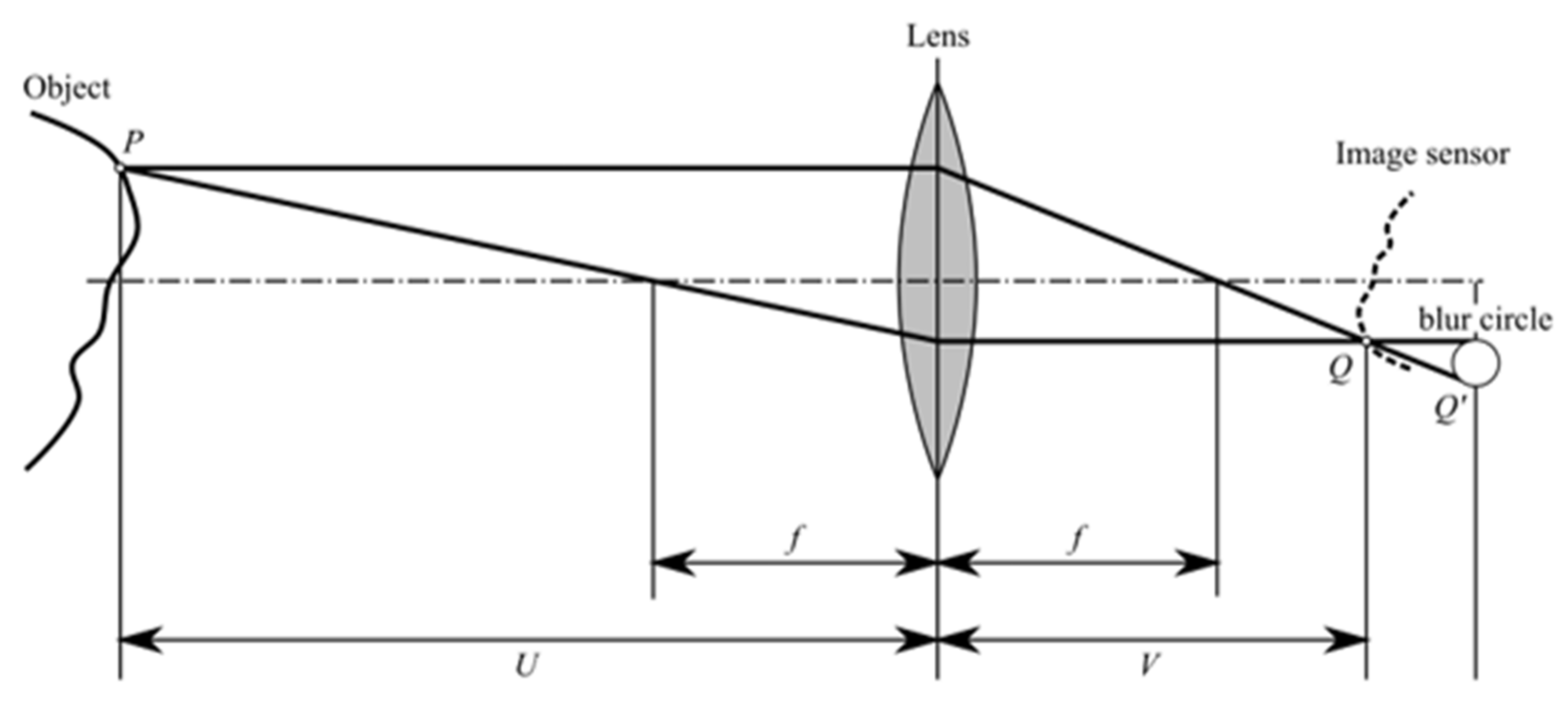
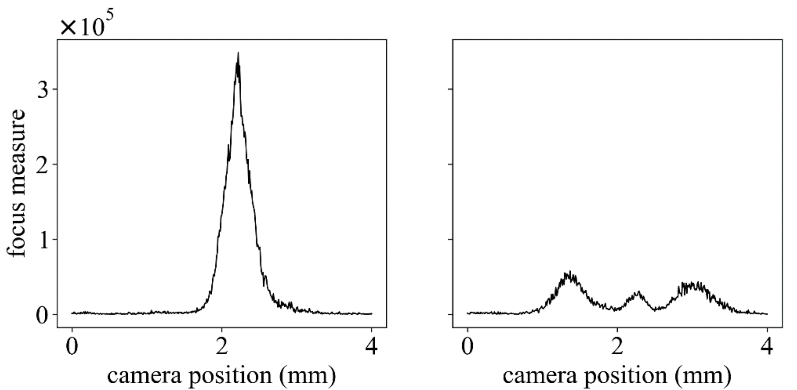
2.1. Shape-from-Focus

Figure 1 shows the principles of imaging in focused and defocused conditions. Let P be a point on the surface of the object. Its focused image is obtained at Q on the image plane. Then, the distance between the lens and the point U, and the distance between the lens and the image plane V, have the following relationship, using the focal length f as:

$$\begin{array}{c}\frac{1}{U}+\frac{1}{V}=\frac{1}{f}\end{array}$$

(1)

Meanwhile, a defocused image is obtained at Q’. The blurring effect is generally modeled by the point spread function (PSF) as:

$$\begin{array}{c}h\left(x,y\right)=\frac{1}{2\pi {\sigma }^2}\exp \left(-\frac{x^2+y^2}{2{\sigma }^2}\right)\end{array}$$

(2)

Then, image formation is the convolution of the actual image $I\left(x,y\right)$ and PSF, as in:

$$\begin{array}{c}{I}^{\prime }\left(x,y\right)=h\left(x,y\right)\times I\left(x,y\right).\end{array}$$

(3)

To change the focus of the camera, the camera, the image sensor, or the lens is translated to the depth direction, and images are captured at each step. To find the focused position U of each pixel, a focus measure expressing the degree of focus is calculated for each pixel in captured frames. One type of focus measure is the Laplacian of Gaussian (LoG), working as a bandpass filter:

$$\begin{array}{c}LOG\left(x,y\right)=\frac{1}{\pi {\sigma }^4}\left(1-\frac{x^2+y^2}{{\sigma }^2}\right)\exp \left(-\frac{x^2+y^2}{2{\sigma }^2}\right)\end{array}$$

(4)

The focus measure $f_{\mathrm{m}}$ at a pixel is obtained by the convolution of Equations (3) and (4) as:

$$\begin{array}{c}{f}_{\mathrm{m}}\left(x,y\right)=LOG\left(x,y\right)\times I^{\prime }\left(x,y\right)\end{array}$$

(5)

The depth of each pixel can be determined as being the camera position that provides the maximum focus measure. In addition to the three-dimensional shape of the object, the focused texture of the object is obtained from each pixel value of the maximum focus measure. Therefore, the SFF process provides a three-dimensional textured surface for the object.

2.2. Experimental Setup

The experimental system, shown in Figure 2, consists of a monochrome digital camera (STC-MB202USB, OMRON SENTECH) with a resolution of 1600 × 1200 pixels, a telecentric lens (35/8/0.1, Carl Zeiss, Wetzlar, Germany), and a triangular prism object with a 10-degree slope. Five sine patterns with different frequencies were prepared and pasted to the object. Figure 3 shows one of the texture patterns. The camera was mounted on a linear actuator (OSMS20-85, SIGMAKOKI) that has a minimum movement of 1 μm. The camera and the actuator were connected to a Windows workstation and were controlled using in-house software written in Python. For the computation of the focus measure, the LoG focus measure was employed.

As for the measurement, the camera was moved from a too-near defocused position to a too-far away defocused position at 0.1 mm intervals, and the camera position and image were recorded at each position. After the measurements, the focus measure at each pixel was computed; then, the depth of each pixel was obtained from the camera position, giving the maximum focus measure.

3. Experiments

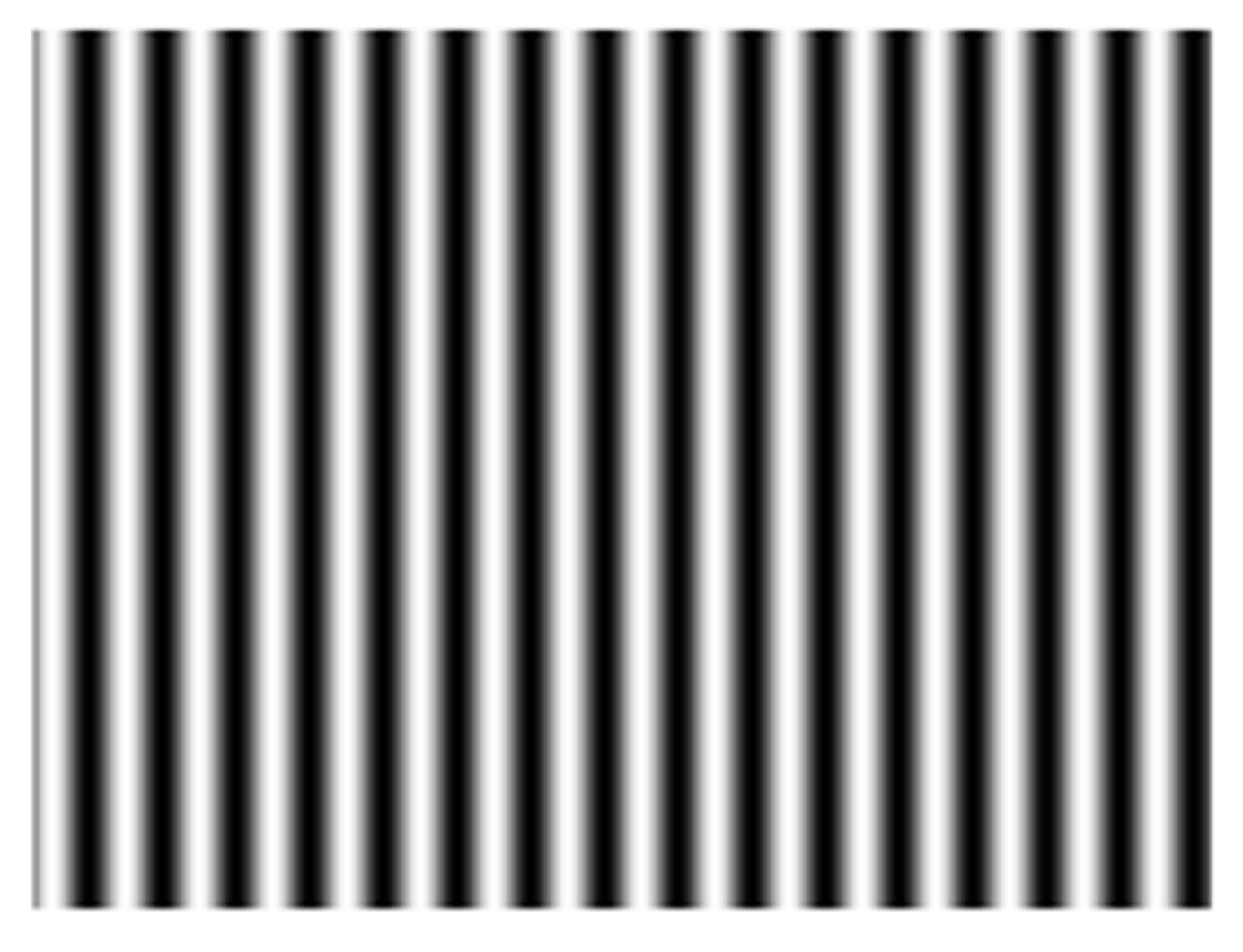
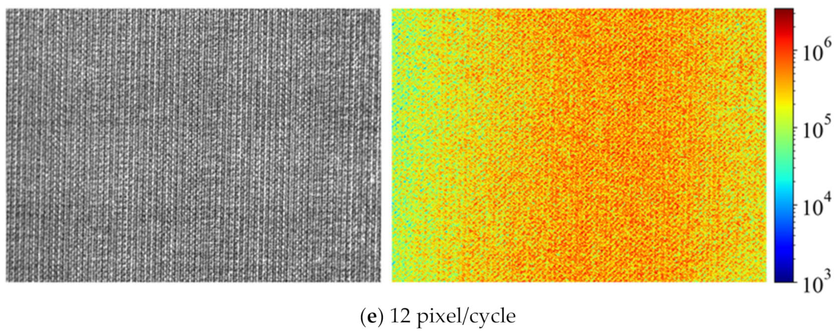
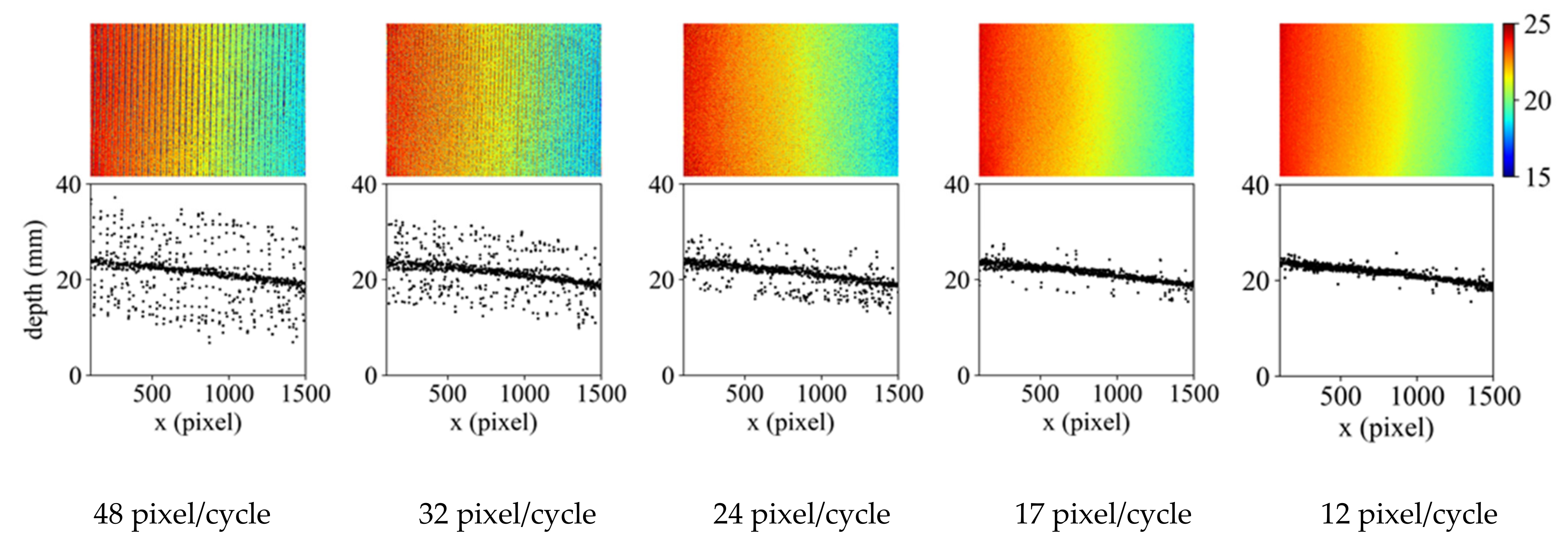
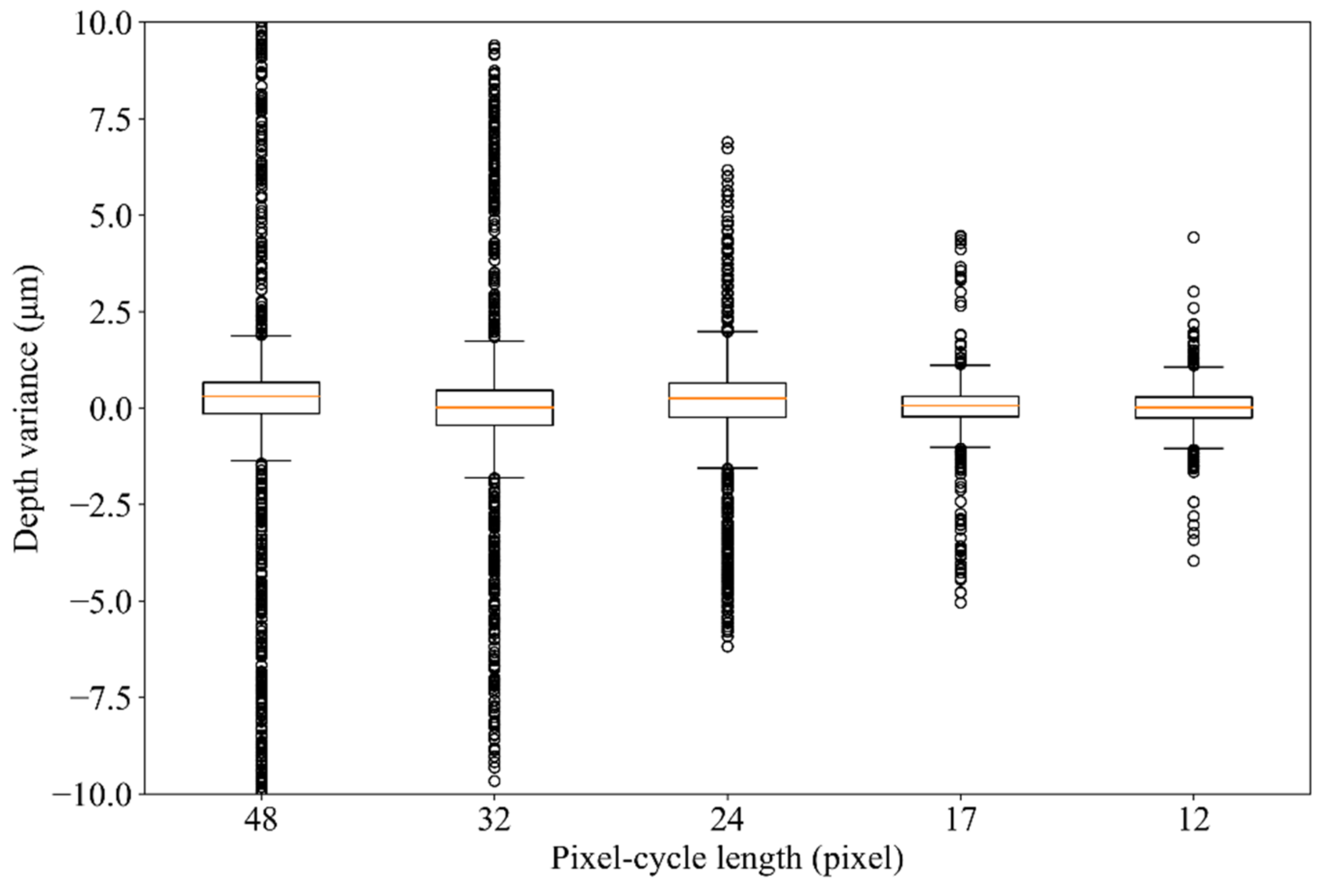
3.1. Precision Validation by Texture Frequencies

Shape measurement precision at various texture frequencies was experimentally investigated. The pixel-cycle lengths of the captured images were 48, 32, 24, 17, and 12 pixels. For each texture, the depth map was generated from the camera positions, giving the maximum focus measure. Figure 4 shows the samples of the captured pictures and their focus measure maps at the relative focused camera positions. In the rough textures, very low-focus measure areas were observed, even in the focused images overall.

Figure 5 shows that the generated depth maps in the upper row and the depths at y = 600 (pixels) in the lower row. The texture frequency increased from the left to the right panel. The depth measurement precision was analyzed by linear regression.

Table 1. Standard errors of regression at each cycle length.

Cycle Length (Pixel/Cycle)	48	32	24	17	12
Std. Err. (mm)	4.18	2.80	1.68	0.86	0.60
Coefficient of Determination	0.11	0.19	0.47	0.75	0.86

shows the standard errors of regression and their coefficient of determination for each cycle length. In all frequencies, the regression lines had good consistency, and the correctness was not different. Meanwhile, the determination coefficients increased with the increasing texture frequency. Figure 6 shows the distributions of the residues in each texture as a boxplot. Despite the fact that the boxes and whiskers, expressing 1.5 times the interquartile range (IQR), were almost the same size in all texture frequencies, the ranges of the outliers depended on the texture frequencies. Hence, the focus measures in the camera position were investigated at the pixels of the small and large residues of the regression, as shown in Figure 7. In an outlier, the focus measure, which did not have one strong peak at the focal position, was not an appropriate value.

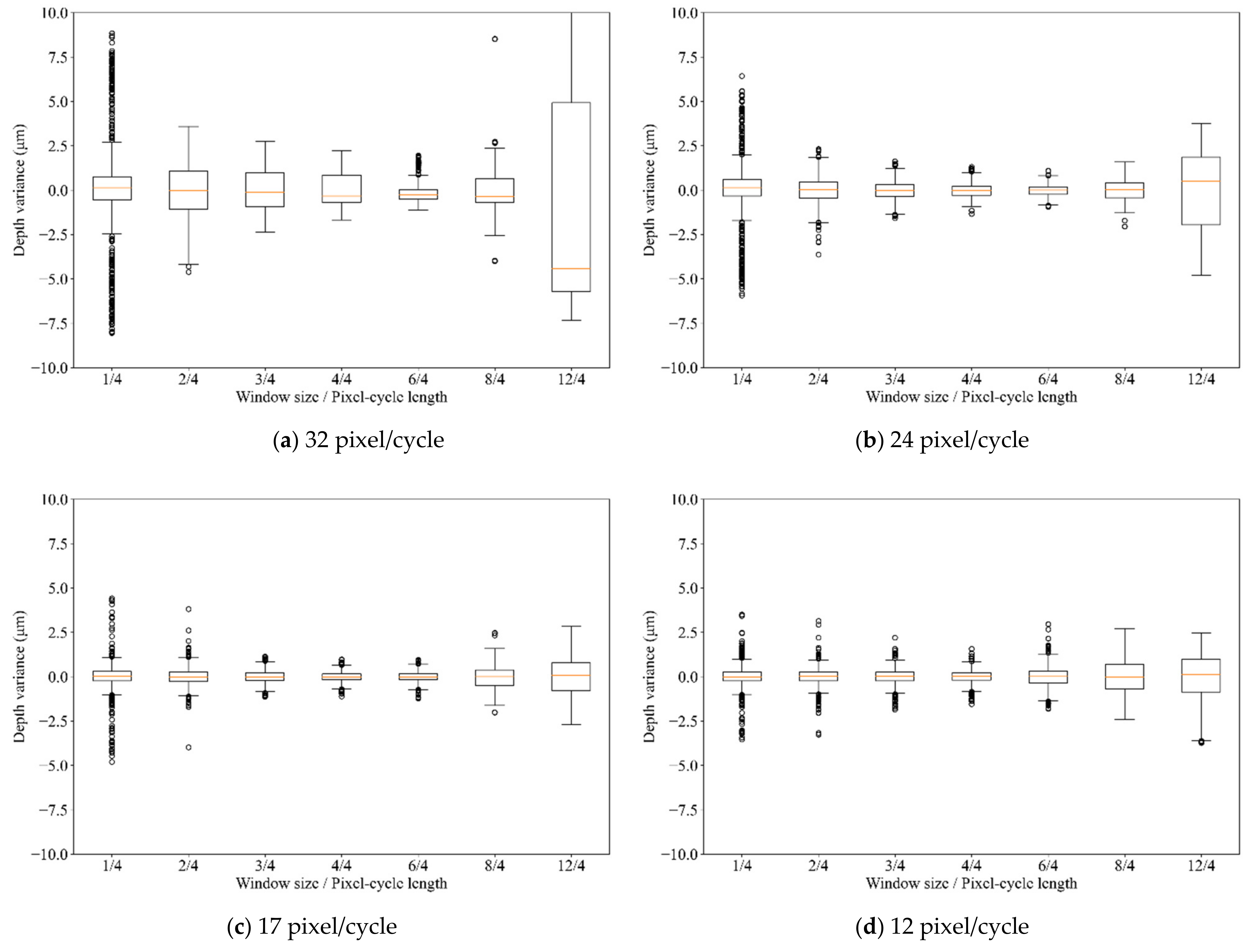
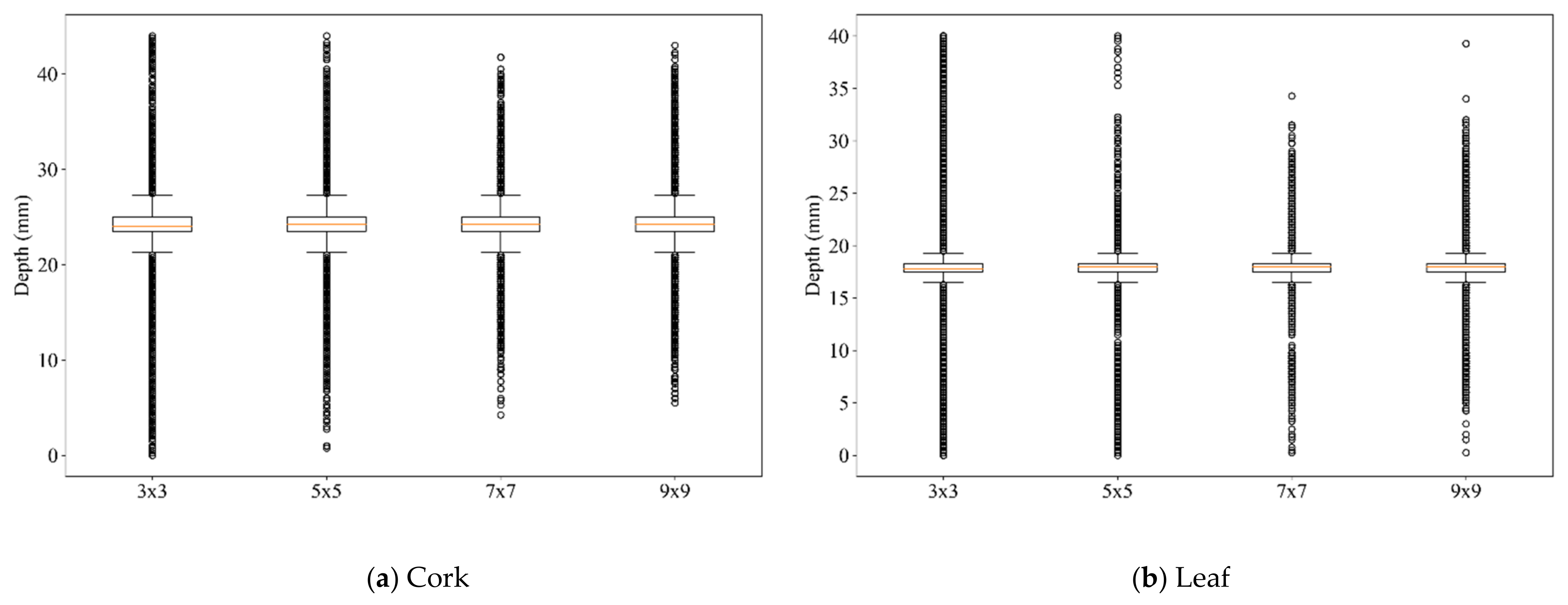
3.2. SFF Precision by Window Size

From the above validation, in the SFF precision, the window size of the focus measure operator might be related to the pixel-cycle length of a texture. To clarify the hypothesis, SFF precisions with the various window sizes were validated. The window sizes were set at from 1/4 to 12/4 times the cycle lengths, as shown in

Table 2. The windows size for each pixel-cycle length of the textures.

Cycle Length (Pixel)	Window Size
	$1/4\mathit{\lambda }$	$2/4 \mathit{\lambda }$	$3/4 \mathit{\lambda }$	$4/4 \mathit{\lambda }$	$6/4 \mathit{\lambda }$	$8/4 \mathit{\lambda }$	$12/4 \mathit{\lambda }$
12	3 × 3	7 × 7	9 × 9	13 × 13	19 × 19	25 × 25	37 × 37
17	5 × 5	9 × 9	13 × 13	17 × 17	25 × 25	35 × 35	51 × 51
24	7 × 7	13 × 13	19 × 19	25 × 25	37 × 37	49 × 49	73 × 73
32	9 × 9	17 × 17	25 × 25	33 × 33	49 × 49	65 × 65	97 × 97

.

Figure 8 shows the depth maps and the depths in the x-axis direction for each texture and each window size. The texture pixel-cycle length increases from the top to the bottom rows, and the window size increases from the left to the right columns.

Overall, the same trend was observed, regardless of the texture. The precision was highest around the window size relative to the 4/4 pixel-cycle length; outliers increased at the smaller window size rather than the cycle length, as in the first experiment, and the depth estimation was more unstable at the larger window size than the cycle length. The trend was observed in Figure 9, which shows the distributions of the residues of linear regression. Except for the result of the 32 pixel-cycle length, the highest precision was achieved for the window size that was equal to the pixel-cycle length.

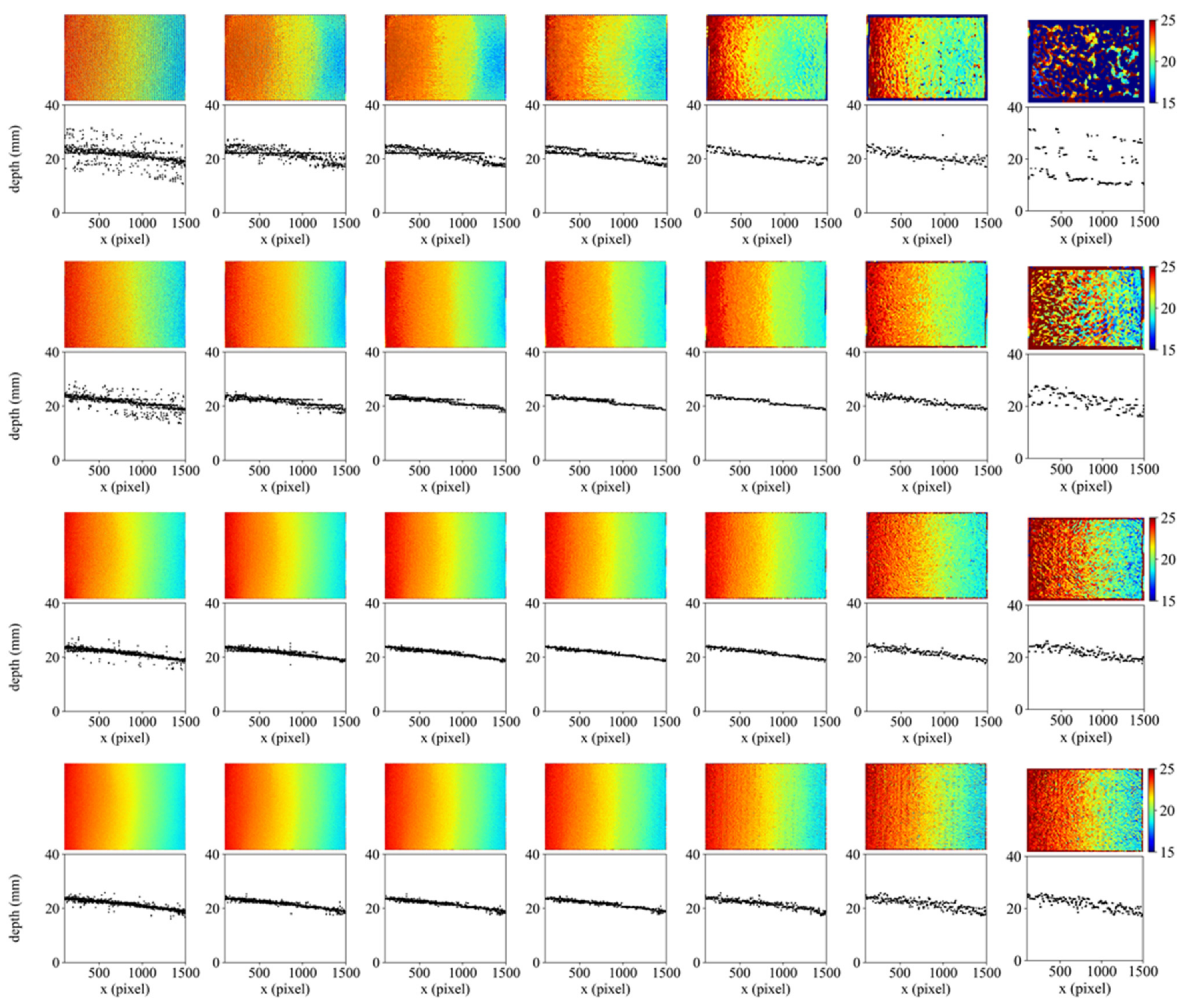
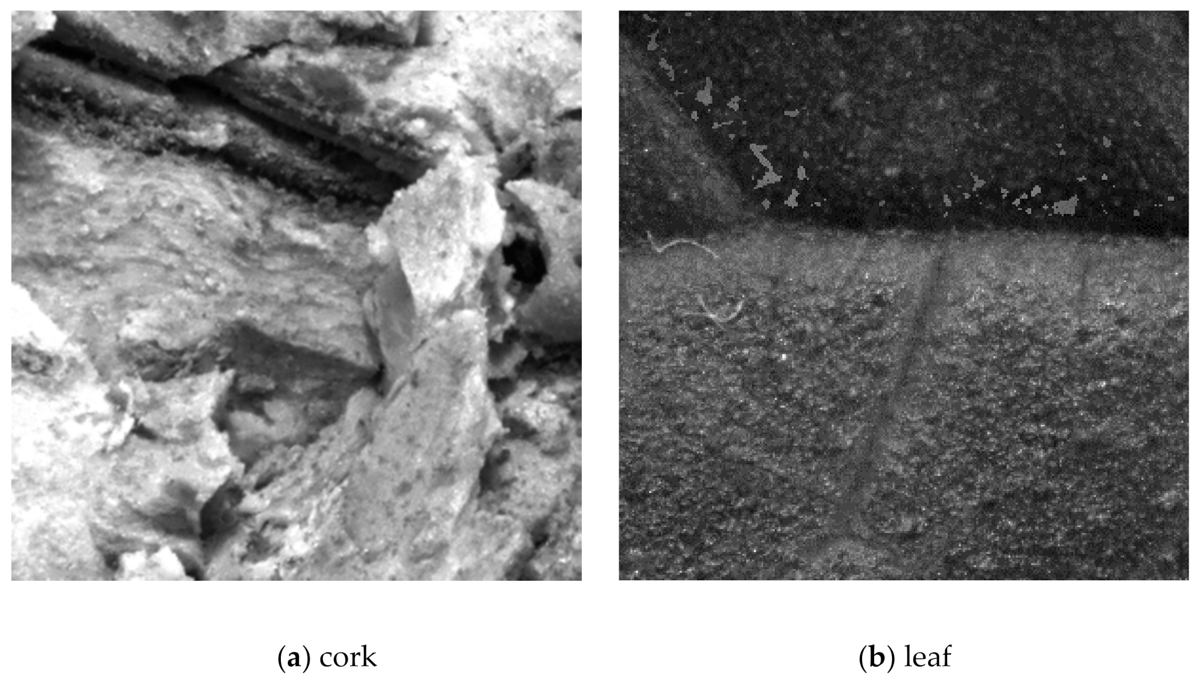
3.3. Qualitative Tests with Real Objects

To support the above findings, qualitative tests with real objects (a broken cork and a leaf) were performed, as shown in Figure 10. The height ranges of the actual objects were 2–3 mm. Window sizes from 3 × 3 to 9 × 9 were applied for shape reconstruction. The reconstructed shapes are shown in Figure 11. The depth variations of the respective objects are shown in Figure 12. From the results, the outlier ranges were minimized in the 7 × 7 window size. This suggests that the texture had 7 pixel-cycle length components.

4. Discussion

We investigated the precision of shape-from-focus imaging according to the texture frequency. The experimental results revealed two considerations. Firstly, the window size of the focus measure operator should be adjusted with the pixel-cycle length of a texture in order to compute the focus measure correctly. Secondly, the precision of shape-from-focus depends on the texture frequency. Thus, the results suggested that the window size should be adjusted for a local texture frequency. When the window size is smaller than a pixel-cycle length, there are certain pixels at which the Laplacian values are approximately zero. Therefore, their focus measures also have a very small value, even if focused pixels are shown as outliers. On the other hand, when using a large window size, the precision was decreased overall. Too many pixels were used for the focus measure computation; as a result, the residues were uniformly increased. Therefore, dynamic adjustment of the window size is needed. Regarding the optimization of the window size, several studies have been reported; however, they did not focus on texture frequencies. Our findings could have the potential to adjust the window size based on local texture frequencies.

Regarding the limitations of this study, sine wave patterns with a single frequency were used for the textures; however, real objects have various frequencies and amplitudes. The effect of amplitude at each frequency on the precision of shape measurement needs to be studied in the future. Moreover, this study used a telecentric lens, which does not have a magnification shift. To apply the technique with a general lens system, compensation for magnification shift [11] is required for correct focus measure computation.

As mentioned in the Introduction, other focus measure operators have been proposed. However, it was not clear whether the results can apply to other focus measures because this study was designed for an LoG filter, which works as a bandpass filter. Theoretically, the trend should be similar, since a small window size is considered to have more precision but less robustness, while a large window size is considered to have more robustness but less precision; however, its investigation is left for future work.

5. Conclusions

In this study, we investigated the precision of shape-from-focus measurement by texture frequencies. In the first experiment, the depth was measured with the fixed window size for various pixel-cycle length textures. Many outliers were observed in a depth map because a focus measure was not computed correctly. Therefore, we consider that it is one cause of depth measurement noise in shape-from-focus. In the second experiment, the depth was measured with the window sizes related to the pixel-cycle lengths. The variations of the measurement errors were different less or more than the pixel-cycle lengths. When the window size was smaller than the pixel-cycle length, outliers were observed as in the first experiment. Meanwhile, when the window size was larger than the cycle length, the variation was overall increased. The results suggested the window size equal to the pixel-cycle length of a texture might measure the depth precisely. The findings would potentially contribute to determining the appropriate window size of the focus measure operator in shape-from-focus reconstruction.

References

1. Thanusutiyabhorn, P.; Kanongchaiyos, P.; Mohammed, W. Image-based 3D laser scanner. In Proceedings of the 8th Electrical Engineering/Electronics, Computer, Telecommunications and Information Technology (ECTI) Association of Thailand—Conference 2011, Khon Kaen, Thailand, 17–19 May 2011; Institute of Electrical and Electronics Engineers (IEEE): Piscataway, NJ, USA, 2011; pp. 975–978. [Google Scholar]
2. Nayar, S.K.; Nakagawa, Y. Shape from focus. IEEE Trans. Pattern Anal. Mach. Intell. 1994, 16, 824–831. [Google Scholar] [CrossRef] [Green Version]
3. Takeshita, T.; Kim, M.; Nakajima, Y. 3-D shape measurement endoscope using a single-lens system. Int. J. Comput. Assist. Radiol. Surg. 2012, 8, 451–459. [Google Scholar] [CrossRef]
4. Thelen, A.; Frey, S.; Hirsch, S.; Hering, P. Improvements in Shape-From-Focus for Holographic Reconstructions With Regard to Focus Operators, Neighborhood-Size, and Height Value Interpolation. IEEE Trans. Image Process. 2008, 18, 151–157. [Google Scholar] [CrossRef] [PubMed]
5. Groen, F.; Young, I.; Ligthart, G. A comparison of different focus functions for use in auto focus algorithms. Cytometry 1985, 6, 81–91. [Google Scholar] [CrossRef] [PubMed] [Green Version]
6. Yeo, T.; Ong, S.; Jayasooriah; Sinniah, R. Autofocusing for tissue microscopy. Imag. Vis. Comput. 1993, 11, 629–639. [Google Scholar] [CrossRef]
7. Pertuz, S.; Puig, D.; Garcia, M.A. Analysis of focus measure operators for shape-from-focus. Pattern Recognit. 2013, 46, 1415–1432. [Google Scholar] [CrossRef]
8. Malik, A.S.; Choi., T.S. Consideration of illumination effects and optimization of window size for accurate calculation of depth map for 3D shape recovery. Pattern Recognit. 2007, 40, 154–170. [Google Scholar] [CrossRef]
9. Marshall, J.; Burbeck, C.; Ariely, D.; Rolland, J.; Martin, K. Occlusion edge blur: A cue to relative visual depth. J. Opt. Soc. Am. A 1996, 13, 681–688. [Google Scholar] [CrossRef] [PubMed] [Green Version]
10. Lee, I.; Mahmood, M.T.; Choi, T.S. Adaptive window selection for 3D shape recovery from image focus. Opt. Laser Technol. 2013, 45, 21–31. [Google Scholar] [CrossRef]
11. Pertuz, S.; Puig, D.; García, M.Á. Improving Shape-from-Focus by Compensating for Image Magnification Shift. In Proceedings of the 2010 20th International Conference on Pattern Recognition, Istanbul, Turkey, 23–26 August 2010; Institute of Electrical and Electronics Engineers (IEEE): Piscataway, NJ, USA, 2010; pp. 802–805. [Google Scholar]
Figure 1. Principles of an optical system.
Electronics 10 01870 g001
Figure 2. Experimental setup.
Electronics 10 01870 g002
Figure 3. One of the prepared textures.
Electronics 10 01870 g003
Figure 4. Captured pictures (left) and their focus measure maps (right) for each pixel-cycle length.
Electronics 10 01870 g004aElectronics 10 01870 g004b
Figure 5. Results of the 3-D depth measurements by the various pixel-cycle lengths of the textures. The upper part shows the depth map of the reconstructed shape, and the lower part shows the x-z plane (y = 600) of the reconstructed shape.
Electronics 10 01870 g005
Figure 6. Residual distribution of regression in each cycle length, shown in a boxplot. The median is depicted by the orange line inside each box, and the interquartile range (IQR) is depicted by the length of the box. The whiskers correspond to 1.5 IQRs. The circles indicate outliers.
Electronics 10 01870 g006
Figure 7. Focus measure distributions at the pixels in the small residue (left) and the large residue (right).
Electronics 10 01870 g007
Figure 8. Results of depth measurements: 12 pixels (first row), 17 pixels (second row), 24 pixels (third row), 32 pixels (bottom), 1/4 λ (first column), 2/4 λ (second column), 3/4 λ (third column), 4/4 λ (fourth column), 6/4 λ (fifth column), 8/4 λ (sixth column), 12/4 λ (seventh column).
Electronics 10 01870 g008
Figure 9. Residual distribution at each window size for each pixel-cycle length.
Electronics 10 01870 g009
Figure 10. Real objects for qualitative tests. (a) A broken cork, (b) a leaf.
Electronics 10 01870 g010
Figure 11. Depth map of the real objects (Upper: cork, lower: leaf).
Electronics 10 01870 g011
Figure 12. Depth distributions of the window sizes. In the 7 × 7 window size, the outliers were slightly reduced.
Electronics 10 01870 g012