Offloading Data through Unmanned Aerial Vehicles: A Dependability Evaluation

Abstract

Applications in the Internet of Things (IoT) context continuously generate large amounts of data. The data must be processed and monitored to allow rapid decision making. However, the wireless connection that links such devices to remote servers can lead to data loss. Thus, new forms of a connection must be explored to ensure the system’s availability and reliability as a whole. Unmanned aerial vehicles (UAVs) are becoming increasingly empowered in terms of processing power and autonomy. UAVs can be used as a bridge between IoT devices and remote servers, such as edge or cloud computing. UAVs can collect data from mobile devices and process them, if possible. If there is no processing power in the UAV, the data are sent and processed on servers at the edge or in the cloud. Data offloading throughout UAVs is a reality today, but one with many challenges, mainly due to unavailability constraints. This work proposes stochastic Petri net (SPN) models and reliability block diagrams (RBDs) to evaluate a distributed architecture, with UAVs focusing on the system’s availability and reliability. Among the various existing methodologies, stochastic Petri nets (SPN) provide models that represent complex systems with different characteristics. UAVs are used to route data from IoT devices to the edge or the cloud through a base station. The base station receives data from UAVs and retransmits them to the cloud. The data are processed in the cloud, and the responses are returned to the IoT devices. A sensitivity analysis through Design of Experiments (DoE) showed key points of improvement for the base model, which was enhanced. A numerical analysis indicated the components with the most significant impact on availability. For example, the cloud proved to be a very relevant component for the availability of the architecture. The final results could prove the effectiveness of improving the base model. The present work can help system architects develop distributed architectures with more optimized UAVs and low evaluation costs.

1. Introduction

The number of applications for mobile devices has been increasing rapidly. These applications include video streaming, augmented reality applications, audio/video conferences, collaborative editing, etc. [1]. These applications usually require a lot of computational resources, but run on devices with limited resources. Alternatively, instead of performing such a task on a mobile device, a request can be made for the execution to take place on a remote computer; this is called offloading [2]. According to the Statista (a German online portal for statistics), the number of mobile devices will be around 17.72 billion in 2024 [3]. However, mobile devices are often located in areas with a poor internet connection. New network architectures must be devised to mitigate this problem.

Recently, a new architectural possibility for extending resources using unmanned aerial vehicles (UAVs) has emerged [4,5,6,7,8]. UAVs can collect data from mobile devices and process them, if possible. If there is no processing power in the UAV, the data are sent and processed on servers at the edge or in the cloud. UAVs have some advantages, such as easy implementation and low acquisition cost [8]. Implementing universal coverage for the collection, dissemination, and retransmission of wireless data opens up a range of application possibilities for various problems. UAVs can act on this problem as mobile infrastructures functioning as a bridge between mobile devices and terrestrial processing structures. Mobile devices can include sensors and actuators from the Internet of Things (IoT) context. IoT applications are often of an emergency nature, requiring high availability and low latency. Despite the advantages of using UAVs for offloading, these systems can face failures at several points, thus compromising different contexts’ monitoring. Thus, it becomes necessary to evaluate these systems’ availability with UAVs, even before implementing a real infrastructure.

Among the various existing methodologies, stochastic Petri nets (SPN) provide models that represent complex systems with different characteristics. SPNs can represent parallelism, concurrency, and simultaneity, and can be used to evaluate various types of systems [9,10,11]. In the context of UAVs, some related works have already used Petri nets. Lundell et al. [12] adopted Fuzzy Petri nets to evaluate UAV decision making. Gonçalves et al. [13] assessed vehicle safety monitoring issues, using Petri nets. More recently, Mehta et al. [14] proposed colored Petri nets to simulate communication between multiple UAVs. However, they did not explore edge or cloud computing, and did not investigate data offloading issues in the context of UAVs.

This paper proposes stochastic Petri nets (SPN) models to assess the dependability of an architecture composed of UAVs and edge and cloud devices, which work together to perform data offloading. Dependability is a metric that encompasses other metrics [15]. A system’s dependability can be understood as its ability to deliver a specified functionality that can be justifiably trusted [16]. In this work, two metrics are adopted: availability and system reliability. Therefore, the main contributions of this paper are as follows:

• Two SPN models (base and extended), which represent and evaluate an architecture based on IoT sensors, UAVs and remote resources, aided by the cloud. The models are highly configurable, as it is possible to calibrate ten timed transitions in the extended model. The models enable system designers to evaluate the studied system according to availability and reliability aspects.
• A sensitivity analysis, which identify the critical points of the architecture, as well as ways to improve it.
• Case studies that provide a practical guide for analyzing the dependability of the proposed architecture. The first case study investigates distinct scenarios for evaluating availability, and the second one focuses on reliability.

The remainder of the paper is divided as follows. Section 2 shows related works. Section 3 provides a detailed explanation of Petri nets and other issues. Section 4 presents the evaluated architecture. Section 5 reveals the availability and reliability models for the proposed architecture. Section 6 presents the results of a case study.

Finally, Section 7 outlines some conclusions and future directions of this work.

2. Related Works

In this section, some works that are related to this paper are presented.

Table 1. Related Works.

Work	Context	Metric	Type of Model	Offloading Application?	Use of Cloud/Edge	Sensitivity Analysis
[13]	Security	Collisions and Forced Landings	Petri Net	No	No	No
[17]	Route Planning	Distance between UAVs	Colored Petri Net	No	No	No
[18]	Malfunction detection	Possibilities of error identification and Reliability	Hierarchical Context-Aware Aspect-Oriented Petri Net	No	No	Yes
[19]	Collision avoidance and location	Memory and decision time	Hierarchical Context-Aware Aspect-Oriented Petri Net	No	No	No
[20]	Fault detection	Abnormality rate in components	Fuzzy Petri Net	No	No	No
[21]	Security	Security level	Colored Petri Net	No	No	No
[22]	Multi-task offloading	Reliability	Markov Decision Process	Yes	Yes	No
[23]	Offloading and Consumption Reduction	Performance	Markov Decision Process with Reinforcement Learning	Yes	Yes	No
[24]	Multiprocess Offloading	Performance	Markov Decision Process with Reinforcement Learning	Yes	Yes	No
This work	Offloading using UAVs	Availability and Reliability	Stochastic Petri Net and RBD	Yes	Yes	Yes

shows the related works under six aspects: context, metrics, model type, offloading application, use of cloud/edge, and sensitivity analysis.

The first comparison criterion is context.For the context, there is a wide range of subjects. Only our work explores UAVs for offloading. Refs. [13,21] presented the most similar proposals and focused on ensuring that UAVs work with a certain level of security, being more focused on hardware and software, respectively. Gonçalves et al. [13] performed an analysis that assesses the safety of UAVs in order to facilitate the airworthiness certification process of UAVs. In this way, the work helps manufacturers to more easily identify critical points in a UAV during development. Zhou et al. [21] generated a model capable of identifying components that do not comply with the established safety requirements, in addition to an algorithm that is also capable of detecting inconsistent components that do not comply with the safety standard. The study of Sharma et al. [18] can be considered the closest to our context, with similarities between measuring reliability and seeking to detect system flaws. However, the work has a greater focus on evaluating the embedded system that controls devices, such as a UAV, than the UAVs themselves.

The second criterion is metrics. The metrics here are quite different from each other, but others have a very different goal. This is the case of the metrics used by [19,23,24]. These works have a general objective related to performance. For example, Sharma et al. [19] brought forth several metrics that seek to measure the efficiency of a UAV, instead of the more usual metrics of response time and utilization. Cheng et al. [23], on the other hand, already conducted an analysis aimed at measuring computational delay in a data offloading scenario, using UAVs and satellites. Finally, Faraci et al. [24] made a very thorough performance analysis of a scenario similar to the one in this article. The work uses both key performance metrics and efficiency metrics, which makes it different from this article, which measures system availability and reliability. While the other works present metrics that can be associated with the system’s dependability concerning the availability metric, our work stands alone in this sense.

The third criterion is the type of model chosen to evaluate the system. Most papers chose Petri nets [25] and/or with hierarchical models [26] to evaluate their systems. The variation of types observed for the used Petri nets is considerable, ranging from colored Petri nets to Hierarchical Context-Aware Aspect-Oriented Petri nets. However, our work is the only one to use stochastic Petri nets. Some papers also chose to use the Markov decision process to model the system. Chen et al. [22], for example, used the Markov decision process to meet the needs of the practical application scenario and provide a flexible and effective discharge mode.

The fourth and fifth criteria are related, which are the offloading application and use of cloud/edge; as their values are equal, it is worth joining the analysis. The works [22,23,24] were the only ones that approached the proposal presented here. Chen et al. [22] presented a strategy of data retransmission and edge computing in which UAVs simultaneously perform data processing and offloading. Ref. [23] proposed a flexible method of joint computing that provides full cloud/edge computing services to remote IoT users. Finally, Ref. [24] aimed to extend the capabilities of a 5G network to ensure ultra-low latency in processing data streams generated by connected devices. The last criterion is the sensitivity analysis. Our work is the only one that used a sensitivity analysis to check the importance of the components.

3. Background

This section presents the main essential concepts to understand the proposals.

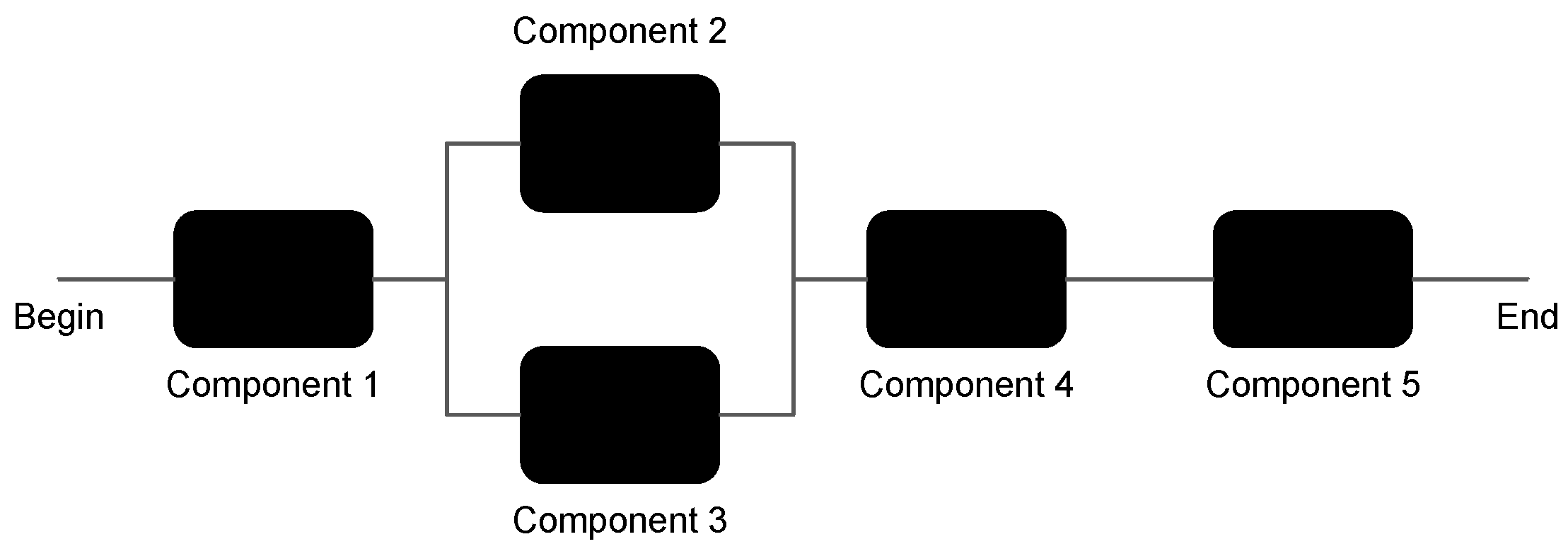
3.1. Reliability Block Diagram

The reliability block diagram (RBD) is a graphical analysis technique that expresses the system as connected components, according to its logical relationship of reliability [27]. In an RBD, the system components and their relations are represented by connections and blocks. The blocks represent the smallest entities in the system, which cannot be further divided: system components or groups of components [28].

In summary, we have a block model, where the connections between them represent a specific system’s behavior. The connections can express two types of behaviors for the components: serial and parallel connections. Components connected in series means that they all must be working for the system to work. When connected in parallel, at least one of the components must be working for the system to be available [29,30,31].

Figure 1 shows an example of an RBD model composed of Components 1 to 5. At the beginning of the model, we have Begin; it represents the beginning of the system, usually followed by the lowest parts of the evaluated system. At the end of the model, we have End; it represents the end of the system, which is usually closer to the highest parts of the evaluated system, which can be several things, such as an operating system, software, virtual machine, etc. In the model, we have, in principle, series connections and a parallel connection. In this RBD example, the system is operational if components 1, 4, and 5 are working, and components 2 or 3 are active. An RBD model’s reliability analysis depends on the mean time to recover (MTTR) and mean time to failure (MTTR) of each component in the system.

3.2. Stochastic Petri Net

SPNs [32,33,34,35,36,37,38] can be identified as a type of directed graph divided into two parts, filled by three types of objects. These objects are places, transitions, and directed arcs that connect places for transitions and transitions to places. Figure 2a illustrates two types of transitions (timed and immediate). The timed transition follows a stochastic behavior, following a probability distribution function. The immediate transition fires when it is activated, without waiting for any period. The white circle symbolizes places. Arcs are used to connect places to transitions. Inhibitory arcs block or allow the passage of tokens from one place to another. Moreover, the token is assigned to a specific place.

In SPN models, to assess availability, the concept of active or inactive components is active. Figure 2b presents a small availability model with two components (A and B). Both have mean failure (MTTF) and repair (MTTR) times. Component A, for example, is active when it has a token in place A_U and is inactive when it has a token in place A_D. In this example, for component B to be active, A must also be active. The inhibiting arc ensures that if component A changes from the upstate to the downstate, the T0 transition is triggered, and component B is then also in the downstate.

3.3. Sensitivity Analysis with DoE

The sensitivity analysis is a measure of the effect of the given input data about the output data, aiming to outline the weak links of the computer systems and, from then on, seek to adopt a set of techniques that aim to improve these systems in different scenarios [39]. In a way, the sensitivity analysis can provide the necessary security and forward the results within the system administrators’ perspective. In this work, we apply a sensitivity analysis with DoE.

The Design of Experiments (DoE) corresponds to a collection of statistical techniques that deepen the knowledge about the product or process under study [40]. It can also be defined by a series of tests in which the researcher changes the set of variables or input factors to observe and identify the reasons for changes in the output response.

The parameters to be changed are defined using an experiment plan. The goal is to generate the most significant amount of information with the fewest possible experiments. The behavior of the system based on parameter changes can be observed using sets of outputs. In the literature, there are three categories of graphs usually adopted for experiments with DoE:

• The Pareto chart is represented by bars in descending order. The higher the bar, the greater the impact. Each bar represents the influence of each factor on the dependent variable.
• Main effects graphs are used to examine the differences between the level means for one or more factors, graphing the mean response for each factor level connected by a line. It can be applied when using a comparison between the relative strength of the effects of various factors. The signal and magnitude of the main effect can express the mean response value. The magnitude expresses the strength of the effect. The higher the slope of the line, the greater the magnitude of the main effect. It is necessary to consider that the horizontal line means that it has no main effect, that is, each level affects the response in the same way.
• Interaction graphs are responsible for identifying interactions between factors. An interaction occurs when the influence of a given factor on the result is altered (amplified or reduced) by the difference in another factor’s level. Assuming that the lines on the graph are parallel, there is no interaction between the factors. If they are not parallel, there is an interaction between the factors.

4. Evaluated Architecture Overview

Figure 3 shows the base architecture modeled in this work. The architecture consists of a distributed system composed of IoT devices that generate requests to remote servers. There is a chain of UAVs that communicate with a base station that receives such data. The collected data are processed by a cloud or edge server, depending on the demand. Thus, communication takes place in three stages:

• IoT devices are the customers of the application requesting services and sending data. UAVs are controlled via a wireless network (5G, for example). UAVs fly over the communication area, receiving data from mobile devices.
• The base station receives data from UAVs and retransmits them to the cloud.
• The data are processed in the cloud, and the responses are sent back to the IoT devices.

A possible limitation is that the service may become unavailable depending on the data demand. Just one UAV failing can significantly decrease the availability of the system, regarding a critical application. Another possible limitation of the base architecture is that if the cloud goes down, the entire system will stop working. Figure 4 presents a second proposal of the redundant architecture where a server at the edge of the network is added. The goal is to improve availability because, depending on the type of request, processing can be performed at the edge. Both servers are always connected. However, as there are two servers, the load is divided. If the cloud goes down, the edge server takes over the processing and vice versa. The battery and recharge time of the UAV is not taken into account. In Figure 4, the cloud server (3.a) and the edge server (3.b) are a server mounted on a single physical machine.

5. SPN Models

This section presents the proposed models generated for representing the architecture behavior shown in the previous section.

5.1. Base Model

This section presents the SPN base model. The components in the model correspond to the same components shown in the previous section. Figure 5 shows the model with the following functions: (i) UAVs are responsible for collecting data for offloading; (ii) the network is responsible for receiving requests from UAVs and forwarding them to the cloud; and (iii) the cloud is responsible for processing the data. Each component has its respective MTTF and MTTR. The network is modeled, taking into account the dependency between the components. When a component fails, the immediate transition (T0) makes the next component, which depends directly or indirectly on it, also fail.

The ND mark in place UAV_U corresponds to the number of available UAVs. The UAVs are working when the ND tokens are in the UAV_U place. The evaluator can define (with this ND tag) how many UAVs must be active for the system to be working. A UAV component is not working when it has a token in the UAV_D place. The change between the active and inactive states is caused by the transitions UAV_MTTF and UAV_MTTR.

The network is up and running when it has tokens in the NETWORK_U place. The network component is not working when it has a token in one of the following places: BS_D or NETWORK_D. The base station is working if it has a token in the place BS_U; it is inactive when it has a token in the place BS_D. The change between the active and inactive state is caused by the following transitions: BS_MTTF and NETWORK_MTTF for the mean time to failure; and BS_MTTR and NETWORK_MTTR for the mean time to repair.

The cloud is working when it has tokens in the CLOUD_U place. We consider that the cloud component is not working when it has a token in the CLOUD_D place. The change between the active and inactive status is caused by the transitions CLOUD_MTTF and CLOUD_MTTR for the mean time failure and repair, respectively. Especially for the cloud, an RBD model is designed to obtain the failure and recovery times. The RBD model and its data for simulation are based on the model presented by [41].

Figure 6 shows the RBD model used to obtain data from the cloud component. We consider a private cloud type. The components adopted are the same platform components as Eucalyptus or OpenStack. The main components that form a cloud are the frontend and nodes. In order to obtain the failure and recovery values of these components, they are subdivided. The node is formed by the following components: hardware (HW), operating system (OS), hypervisor, instance manager (IM), and virtual machine (VM). The frontend is formed by the following components: hardware (HW), operating system (OS), platform manager (PM), cluster manager (CM), block-based storage (BBS), and file-based storage (FBS).

The metrics used with the base model are availability and downtime. The availability equation represents a sum of probabilities of the number of tokens for each state. Thus, P stands for probability, and # stands for the number of tokens in a given place. The downtime (D) can be obtained by $D=(1-A)\times 8760$, where A represents the system’s availability and 8760, the number of hours in the year. For the availability metric, the system is fully functional when all the UAVs that the system supports, cloud and network, are active at the same time. The availability of the model can be measured in two ways. Equation $A=P\left\{\right(\#$ UAV$\_U=ND\left)AND\right(\#CLOUD\_U>0\left)AND\right(\#NETWORK\_U>0\left)\right\}$ calculates the system availability of the base model when 100% of the UAVs are required to work. Equation $A=P\left\{\right(\#$ UAV$\_U>=MND\left)AND\right(\#CLOUD\_U>0\left)AND\right(\#NETWORK\_U>0\left)\right\}$ calculates the system availability of the base model when a minimum number of UAVs (MND) is required to be working. It is worth mentioning that in order to have a more realistic simulation, the guard condition $\#BS\_U>0$ is used in the transition NETWORK_MTTR so that the network component can only be recovered when the base station is working.

5.2. Sensitivity Analysis with DoE

The first step in conducting a sensitivity analysis with DoE is to define which factors and levels are to be considered. In this work, the base model transitions are adopted as factors, varying each factor in two levels.

Table 2. Factors and respective levels.

Parameter	Level 1	Level 2
BS_MTTF	250,000	750,000
BS_MTTR	1	3
NET_MTTF	41,610	124,830
NET_MTTR	6	18
UAV_MTTF	17,711.7	53,135
UAV_MTTR	0.5	1.5
CLOUD_MTTF	62.94	189
CLOUD_MTTR	0.45	1.37

shows the factors and respective levels.

Table 3. Design of Experiments (all values are in hours).

Scenario	BS_MTTF	BS_MTTR	NET_MTTF	NET_MTTR	UAV_MTTF	UAV_MTTR	CLOUD_MMTF	CLOUD_MTTR
#1	250,000	1	124,830	6	17,711.7	1.5	62.94	0.45
#2	750,000	1	41,610	6	17,711.7	1.5	189.00	1.37
#3	750,000	3	41,610	18	17,711.7	0.5	189.00	1.37
#4	750,000	1	41,610	6	53,135.0	1.5	189.00	0.45
#5	250,000	1	41,610	6	53,135.0	0.5	62.94	0.45
#6	250,000	3	124,830	18	53,135.0	0.5	62.94	1.37
#7	250,000	1	124,830	18	53,135.0	1.5	189.00	0.45
#8	250,000	1	41,610	18	17,711.7	0.5	189.00	0.45
#9	250,000	1	124,830	6	53,135.0	1.5	62.94	1.37
#10	750,000	3	41,610	6	17,711.7	0.5	62.94	0.45
#11	750,000	3	124,830	18	17,711.7	1.5	189.00	0.45
#12	250,000	1	124,830	18	17,711.7	1.5	189.00	1.37
#13	750,000	1	41,610	18	17,711.7	1.5	62.94	0.45
#14	250,000	3	124,830	18	17,711.7	0.5	62.94	0.45
#15	750,000	3	124,830	6	53,135.0	1.5	62.94	0.45
#16	250,000	3	124,830	6	53,135.0	0.5	189.00	0.45
#17	750,000	3	124,830	18	53,135.0	1.5	189.00	1.37
#18	250,000	3	124,830	6	17,711.7	0.5	189.00	1.37
#19	250,000	3	41,610	6	53,135.0	1.5	189.00	1.37
#20	750,000	3	41,610	6	53,135.0	0.5	62.94	1.37
#21	250,000	1	41,610	6	17,711.7	0.5	62.94	1.37
#22	750,000	1	124,830	6	17,711.7	0.5	189.00	0.45
#23	750,000	3	41,610	18	53,135.0	0.5	189.00	0.45
#24	750,000	1	124,830	6	53,135.0	0.5	189.00	1.37
#25	750,000	1	124,830	18	53,135.0	0.5	62.94	0.45
#26	250,000	1	41,610	18	53,135.0	0.5	189.00	1.37
#27	750,000	3	124,830	6	17,711.7	1.5	62.94	1.37
#28	750,000	1	124,830	18	17,711.7	0.5	62.94	1.37
#29	750,000	1	41,610	18	53,135.0	1.5	62.94	1.37
#30	250,000	3	41,610	18	17,711.7	1.5	62.94	1.37
#31	250,000	3	41,610	6	17,711.7	1.5	189.00	0.45
#32	250,000	3	41,610	18	53,135.0	1.5	62.94	0.45

shows the combinations of DoE scenarios generated from the design table.

Figure 7 shows the Pareto graph with the level of significance for each of the factors in the model. The term H is the most significant for the availability variable. This fact corroborates the hypothesis that the cloud is the main element for the base architecture’s availability. It is observed that the term G is raised to almost the same level as the term H. In summary, both the recovery and the cloud’s failure are essential factors for maintaining the system.

Figure 8 shows the level of interaction between the factors CLOUD_MTTR and CLOUD_MTTF. Such factors were the most significant in the study of the impacts on the Pareto chart. The non-parallel lines indicate that there is an interaction between the factors. The result of changing one factor influences the result of changing the second factor. With a lower CLOUD_MTTF, the variation in CLOUD_MTTR has a more significant influence on availability.

Figure 9 shows a Contour graph of the interaction between MTTF and MTTR from the cloud. The Contour graph shows the same information as the interaction graph, but differently, through heat zones. The higher the MTTF and the lower the MTTR, the greater the overall availability of the system. Assuming that the recovery time is over 1.2, the system never reaches more than 99.2% availability.

5.3. Extended Model

Figure 10 presents an extended SPN model for the UAV architecture, with two processing possibilities (edge and cloud), a network, and a UAV component. To satisfy these conditions, two new transitions are added, EDGE_MTTF and EDGE_MTTR, which represent the failure and recovery time of edge. The places EDGE_U and EDGE_D represent the active and inactive states of edge, respectively.

The system’s condition to be fully active is the same as described in the base proposal, with the addition of the edge component. However, as edge represents redundancy for the cloud, it is enough that one of them is active for the system to be available. The availability of the model can be measured in two ways. Equation $A=P\left\{\right(\#$ UAV$\_U=ND\left)AND\right((\#CLOUD\_U>0)$$OR(\#EDGE\_U>0)\left)AND\right(\#NETWORK\_U>0\left)\right\}$ calculates the system availability of the extended model when 100% of the UAVs are required for the system to be working. Equation $A=P\left\{\right(\#$ UAV$\_U>=MND\left)AND\right((\#CLOUD\_U>0)OR(\#EDGE\_U>0)\left)AND\right(\#NETWORK\_U>0\left)\right\}$ calculates the system availability of the extended model when a minimum number of UAVs (MND) are required for the system to be working.

It is worth mentioning that the MTTF transitions are of the infinite server type, and the MTTR transitions are of the single server type, both in the base and in the extended model. In this model, the guard condition $\#BS\_U>0$ is also adopted in the transition NETWORK_MTTR so that the network component can only be recovered when the base station is working.

5.4. Reliability Model

The reliability of a system is a factor that is becoming increasingly decisive for a product to be well accepted by its consumers. Reliability is the conditional probability that a system remains operational given a time interval [0, t], considering that it is operational at t = 0. Three aspects must be taken into account when the reliability of a system or component is analyzed. First, an unambiguous definition of possible system failures must be made. Second, the time unit must be identified, which can be given in hours, days, or cycles of system operation. For example, an operating cycle could be the activation of the engine ignition for an automotive system. The system must be observed under natural operating conditions, subject to real physical conditions. Observing the system under manipulated conditions can generate biased reliability data [42]. Figure 11 shows the reliability model adapted from the base availability model by removing the transitions from MTTR.

As with the availability equations, there are two ways to measure reliability. The equation $R=1-\left(\right(\#BS\_D>0\left)OR\right(\#NETWORK\_D>0\left)OR\right(\#CLOUD\_D>0\left)OR\right(\#$ UAV$\_D>0\left)\right)$ calculates the reliability of the system when 100% of the UAVs need to be active. The equation $R=1-\left(\right(\#BS\_D>0\left)OR\right(\#NETWORK\_D>0\left)OR\right(\#CLOUD\_D>0\left)OR\right(\#$ UAV$\_D>NDD\left)\right)$ calculates the system’s reliability when a minimum number of UAVs needs to be down (NDD). $ND-MND$ can calculate NDD.

The results of this metric are presented over time in the next section from the transient analysis.

6. Case Study

This section presents a case study with the models previously presented. Initially, the parameters used in the simulations are presented. The MTTF and MTTR values for each component are extracted from [43,44,45].

Table 4. Values used in numerical analysis.

Component	MTTF (h)	MTTR (h)
Base Station	500,000	2
Network	83,220	12
UAV	35,423.31	1.5
Cloud	125.89	0.91
Edge	4765.79	3.47

shows the input values of the model components that are adopted for conducting the numerical analysis.

Table 5. Values used in the RBD analysis.

Component	MTTF (h)	MTTR (h)
HW	8760	1.67
OS	2893	0.25
CM	788.4	1
PM	788.4	1
BBS	788.4	1
FBS	788.4	1
Hypervisor	2990	1
+IM	788.4	1
VM	2880	0.019

presents the parameters, extracted from [41], adopted for the RBD analysis.

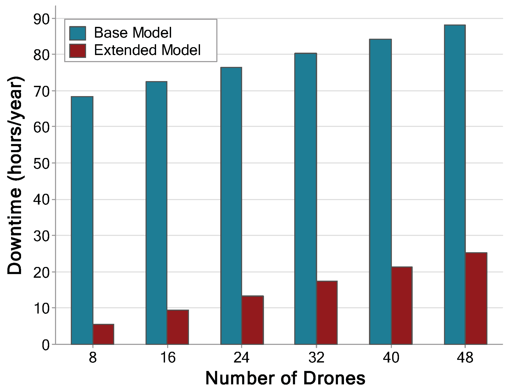
6.1. Results for Availability

This section presents the availability analysis for the two models already presented. Six scenarios are defined, varying the number of available UAVs (8, 16, 24, 32, 40, and 48 UAVs). These scenarios are defined based on the sensitivity analysis of the models. The UAV is a component that appears in the base model as the second most important and as the most important in the extended model. The metric used in the analysis is that 100% of the UAVs need to be active. These scenarios are generated to compare the two models’ availability and the impact that the number of UAVs generates in each of the architectures.

The results calculated by the stationary analysis with the Mercury [46] tool is presented below. Figure 12 shows the availability calculated in the analysis. The availability variation shows that availability drops as UAVs are added to the system. The extended model’s availability tends to fall at better levels than in the base model. We believe that this fact occurs due to the redundancy implemented in the extended model. Even if we add UAVs, there will be a redundant component to supply the cloud’s eventual failures.

Figure 13 shows the downtime in hours per year. The downtime for the extended model tends to be much shorter than that for the base model. The base model ranges from 68 to 88 h/y. The extended model ranges from 5 to 25 h/y. The extended model’s downtime is kept below the base model, even with six times more UAVs, when comparing the base and extended model’s first and last scenarios. The individual values of the base model grow noticeably more and in a linear manner. After the fifth scenario, the time passes 80 h/y, while the extended model remains below thirty. The difference is significant, but both vary approximately 20 h between start and end. It can be deduced that the difference between each scenario is approximately 63 h of downtime reduction.

These results are generally expected since the more components we have in a system, the greater the chances of one of them failing; the more they fail, the more time it takes to fix. As our metric considers the system’s functioning when all UAVs are working, a higher failure rate negatively impacts availability. This behavior is repeated even in the extended model. However, in the extended model, this occurs in a much less impactful way because there is a redundancy mechanism in the server.

6.2. Reliability

Figure 14 shows the reliability of the system over time. For the reliability analysis, three levels of parameters are proposed: CLOUD_MTTF of the base model, CLOUD_MTTF increased by 50%, and CLOUD_MTTF decreased by −50%. The X-axis represents the time sampling in hours. The Y-axis represents the probability of system failure.

The reliability levels are very different from each other. Analyzing the lines at all levels, they follow a decreasing probabilities pattern as the operating time progresses. At the beginning of each test run, each starts with a high probability. Over time they tend to decrease exponentially. As the failure time decreases, there is a tendency for a steeper curve of the line. Such behavior indicates that, with less time between failures, the system tends to fail but decrease in reliability. With the increase between failures, the system tends to fail less frequently during the runtime. Although it seems favorable, this behavior further proves that the base model is not favorable for the recovery and maintenance of the elements. The second conclusion is that cloud failures are harmful, connoting that the cloud is the model’s key element.

6.3. Discussions

The input parameters are adopted mostly from previous works on the studies of generic-purpose UAVs. The computed values are very similar to those from industry (DJI, Parrot, etc.), as we conducted surveys from the internet for general-purpose UAVs. Thus, we believe that the considered UAVs are of general types in industry. Furthermore, one may adopt the proposed models in this work and feed the configurations and parameters of their own UAVs to investigate the dependability output metrics of interest.

It is very interesting to consider the operational conditions of a UAV fleet (e.g., horizontal extent, altitude, and weather). However, the elaboration of the operational conditions is beyond our main focus and out of the research scope in which we investigate the impact of the number of UAVs and operational capacity of components/subsystems on the overall data offloading service dependability (e.g., reliability, availability). We believe the elaboration of different operational conditions is interesting and could provide fruitful research avenue in future works.

7. Conclusions

This paper proposed two SPN models to represent and evaluate a cloud data offloading system’s dependability aided by UAVs. In this work, UAVs were adopted as connection bridges to remote processing resources. The models were highly configurable. The extended model, for example, permitted inserting ten parameters regarding timed transitions. Some scenarios were evaluated by varying the number of UAVs in the system. The availability variation showed that availability dropped as UAVs were added to the system. The extended model’s availability tended to fall at better levels than in the base model. We believe that this fact occurred due to the redundancy implemented in the extended model. By adding redundancy to the model, it was possible to see a considerable increase in availability (about three times) and a large downtime decrease (about seven times). The model analysis was able to identify the most relevant factor in the architecture. The cloud’s MTTR was the factor with greater impact on availability. The analysis also showed the availability behaviour for different recovery and failure times. The reliability model demonstrated the importance of investing in cloud equipment to increase the mean time to failure. As future work, we intend to further extend the model by adding other components, such as distinct internet connections and varied hardware configurations. Other metrics can also be explored, such as security, the drop rate, and the mean response time.

References

1. Hassija, V.; Saxena, V.; Chamola, V. A mobile data offloading framework based on a combination of blockchain and virtual voting. Softw. Pract. Exper. 2020. [Google Scholar] [CrossRef]
2. Meng, X.; Wang, W.; Zhang, Z. Delay-constrained hybrid computation offloading with cloud and fog computing. IEEE Access 2017, 5, 21355–21367. [Google Scholar] [CrossRef]
3. Statista Forecast. Available online: https://www.statista.com/statistics/245501/multiple-mobile-device-ownership-worldwide/ (accessed on 14 February 2021).
4. Feng, W.; Tang, J.; Yu, Y.; Song, J.; Zhao, N.; Chen, G.; Wong, K.K.; Chambers, J. UAV-Enabled SWIPT in IoT Networks for Emergency Communications. IEEE Wirel. Commun. 2020, 27, 140–147. [Google Scholar] [CrossRef]
5. Ye, H.T.; Kang, X.; Joung, J.; Liang, Y.C. Optimization for Full-Duplex Rotary-Wing UAV-Enabled Wireless-Powered IoT Networks. IEEE Trans. Wirel. Commun. 2020, 19, 5057–5072. [Google Scholar] [CrossRef]
6. Liu, Y.; Xie, S.; Zhang, Y. Cooperative Offloading and Resource Management for UAV-Enabled Mobile Edge Computing in Power IoT System. IEEE Trans. Veh. Technol. 2020, 69, 12229–12239. [Google Scholar] [CrossRef]
7. Liu, Y.; Liu, K.; Han, J.; Zhu, L.; Xiao, Z.; Xia, X.G. Resource Allocation and 3D Placement for UAV-Enabled Energy-Efficient IoT Communications. IEEE Internet Things J. 2020, 8, 1322–1333. [Google Scholar] [CrossRef]
8. Tan, Z.; Qu, H.; Zhao, J.; Zhou, S.; Wang, W. UAV-aided Edge/Fog Computing in Smart IoT Community for Social Augmented Reality. IEEE Internet Things J. 2020, 7, 4872–4884. [Google Scholar] [CrossRef]
9. Silva, F.A.; Kosta, S.; Rodrigues, M.; Oliveira, D.; Maciel, T.; Mei, A.; Maciel, P. Mobile cloud performance evaluation using stochastic models. IEEE Trans. Mob. Comput. 2017, 17, 1134–1147. [Google Scholar] [CrossRef]
10. Silva, F.A.; Rodrigues, M.; Maciel, P.; Kosta, S.; Mei, A. Planning mobile cloud infrastructures using stochastic petri nets and graphic processing units. In Proceedings of the 2015 IEEE 7th International Conference on Cloud Computing Technology and Science (CloudCom), Vancouver, BC, Canada, 30 November–3 December 2015; pp. 471–474. [Google Scholar]
11. Marsan, M.A. Stochastic Petri nets: An elementary introduction. In European Workshop on Applications and Theory in Petri Nets; Springer: Berlin/Heidelberg, Germany, 1988; pp. 1–29. [Google Scholar]
12. Lundell, M.; Tang, J.; Nygard, K. Fuzzy petri net for uav decision making. In Proceedings of the 2005 International Symposium on Collaborative Technologies and Systems, St. Louis, MO, USA, 20 May 2005; pp. 347–352. [Google Scholar]
13. Gonçalves, P.; Sobral, J.; Ferreira, L.A. Unmanned aerial vehicle safety assessment modelling through petri nets. Reliab. Eng. Syst. Saf. 2017, 167, 383–393. [Google Scholar] [CrossRef]
14. Mehta, P. A Petri Net Based Simulation for Multiple Unmanned Aerial Vehicles; North Dakota State University: Fargo, ND, USA, 2019. [Google Scholar]
15. Maciel, P.R.; Trivedi, K.S.; Matias, R.; Kim, D.S. Dependability modeling. In Performance and Dependability in Service Computing: Concepts, Techniques and Research Directions; IGI Global: Hershey, PA, USA, 2012; pp. 53–97. [Google Scholar]
16. Laprie, J.C. Dependability: Basic concepts and terminology. In Dependability: Basic Concepts and Terminology; Springer: Berlin/Heidelberg, Germany, 1992; pp. 3–245. [Google Scholar]
17. Fan, L.; Tang, J.; Ling, Y.; Liu, G.; Li, B. Novel conflict resolution model for multi-UAV based on CPN and 4D Trajectories. Asian J. Control 2016, 18, 721–732. [Google Scholar] [CrossRef]
18. Sharma, V.; You, I.; Yim, K.; Chen, R.; Cho, J.H. BRIoT: Behavior rule specification-based misbehavior detection for IoT-embedded cyber-physical systems. IEEE Access 2019, 7, 118556–118580. [Google Scholar] [CrossRef]
19. Sharma, V.; Jayakody, D.N.K.; You, I.; Kumar, R.; Li, J. Secure and efficient context-aware localization of drones in urban scenarios. IEEE Commun. Mag. 2018, 56, 120–128. [Google Scholar] [CrossRef]
20. Liu, J. Knowledge representation and reasoning for flight control system based on weighted fuzzy Petri nets. In Proceedings of the 2010 5th International Conference on Computer Science & Education, Hefei, China, 24–27 August 2010; pp. 528–534. [Google Scholar]
21. Zhou, H.; Zhang, C.; Li, Y.; Gu, Y.; Zhou, S. Verifying the Safety of Aviation Software Based on Extended Colored Petri Net. Math. Probl. Eng. 2019, 2019, 9185910. [Google Scholar] [CrossRef]
22. Chen, Z.; Xiao, N.; Han, D. Multilevel Task Offloading and Resource Optimization of Edge Computing Networks Considering UAV Relay and Green Energy. Appl. Sci. 2020, 10, 2592. [Google Scholar] [CrossRef] [Green Version]
23. Cheng, N.; Lyu, F.; Quan, W.; Zhou, C.; He, H.; Shi, W.; Shen, X. Space/aerial-assisted computing offloading for IoT applications: A learning-based approach. IEEE J. Sel. Areas Commun. 2019, 37, 1117–1129. [Google Scholar] [CrossRef]
24. Faraci, G.; Grasso, C.; Schembra, G. Design of a 5G Network Slice Extension with MEC UAVs Managed with Reinforcement Learning. IEEE J. Sel. Areas Commun. 2020, 38, 2356–2371. [Google Scholar] [CrossRef]
25. Nguyen, T.A.; Kim, D.S.; Park, J.S. Availability modeling and analysis of a data center for disaster tolerance. Future Gener. Comput. Syst. 2016, 56, 27–50. [Google Scholar] [CrossRef]
26. Nguyen, T.A.; Min, D.; Choi, E. A Hierarchical Modeling and Analysis Framework for Availability and Security Quantification of IoT Infrastructures. Electronics 2020, 9, 155. [Google Scholar] [CrossRef] [Green Version]
27. Guo, H.; Yang, X. A simple reliability block diagram method for safety integrity verification. Reliab. Eng. Syst. Saf. 2007, 92, 1267–1273. [Google Scholar] [CrossRef]
28. Čepin, M. Reliability block diagram. In Assessment of Power System Reliability; Springer: Berlin/Heidelberg, Germany, 2011; pp. 119–123. [Google Scholar]
29. Nannapaneni, S.; Dubey, A.; Abdelwahed, S.; Mahadevan, S.; Neema, S. A model-based approach for reliability assessment in component-based systems. In Proceedings of the Annual Conference of the Prognostics and Health Management Society, Fort Worth, TX, USA, 29 September–2 October 2014. [Google Scholar]
30. Kim, M.C. Reliability block diagram with general gates and its application to system reliability analysis. Ann. Nucl. Energy 2011, 38, 2456–2461. [Google Scholar] [CrossRef]
31. Nguyen, T.A.; Min, D.; Choi, E.; Thang, T.D. Reliability and Availability Evaluation for Cloud Data Center Networks using Hierarchical Models. IEEE Access 2019, 7, 9273–9313. [Google Scholar] [CrossRef]
32. Carvalho, D.; Rodrigues, L.; Endo, P.T.; Kosta, S.; Silva, F.A. Mobile Edge Computing Performance Evaluation using Stochastic Petri Nets. In Proceedings of the 2020 IEEE Symposium on Computers and Communications (ISCC), Rennes, France, 7–10 July 2020; pp. 1–6. [Google Scholar]
33. Silva, F.A.; Fé, I.; Gonçalves, G. Stochastic models for performance and cost analysis of a hybrid cloud and fog architecture. J. Supercomput. 2020, 77, 1537–1561. [Google Scholar] [CrossRef]
34. Santos, G.L.; Gomes, D.; Kelner, J.; Sadok, D.; Silva, F.A.; Endo, P.T.; Lynn, T. The internet of things for healthcare: Optimising e-health system availability in the fog and cloud. Int. J. Comput. Sci. Eng. 2020, 21, 615–628. [Google Scholar] [CrossRef]
35. Nguyen, T.A.; Min, D.; Choi, E.; Lee, J.W. Dependability and Security Quantification of an Internet of Medical Things Infrastructure based on Cloud-Fog-Edge Continuum for Healthcare Monitoring using Hierarchical Models. IEEE Internet Things J. 2021. [Google Scholar] [CrossRef]
36. Ferreira, L.; da Silva Rocha, E.; Monteiro, K.H.C.; Santos, G.L.; Silva, F.A.; Kelner, J.; Sadok, D.; Bastos Filho, C.J.; Rosati, P.; Lynn, T.; et al. Optimizing Resource Availability in Composable Data Center Infrastructures. In Proceedings of the 2019 9th Latin-American Symposium on Dependable Computing (LADC), Natal, Brazil, 19–21 November 2019; pp. 1–10. [Google Scholar]
37. Rodrigues, L.; Endo, P.T.; Silva, F.A. Stochastic Model for Evaluating Smart Hospitals Performance. In Proceedings of the 2019 IEEE Latin-American Conference on Communications (LATINCOM), Salvador, Brazil, 11–13 November 2019; pp. 1–6. [Google Scholar]
38. Pinheiro, T.; Silva, F.A.; Fé, I.; Oliveira, D.; Maciel, P. Performance and Resource Consumption Analysis of Elastic Systems on Public Clouds. In Proceedings of the 2019 IEEE International Conference on Systems, Man and Cybernetics (SMC), Bari, Italy, 6–9 October 2019; pp. 2115–2120. [Google Scholar]
39. Campolongo, F.; Tarantola, S.; Saltelli, A. Tackling quantitatively large dimensionality problems. Comput. Phys. Commun. 1999, 117, 75–85. [Google Scholar] [CrossRef]
40. Kleijnen, J.P. Sensitivity analysis and optimization in simulation: Design of experiments and case studies. In Proceedings of the Winter Simulation Conference, Arlington, VA, USA, 3–6 December 1995; pp. 133–140. [Google Scholar]
41. Melo, C.; Matos, R.; Dantas, J.; Maciel, P. Capacity-oriented availability model for resources estimation on private cloud infrastructure. In Proceedings of the 2017 IEEE 22nd Pacific Rim International Symposium on Dependable Computing (PRDC), Christchurch, New Zealand, 22–25 January 2017; pp. 255–260. [Google Scholar]
42. Gillespie, A.M. Reliability & maintainability applications in logistics & supply chain. In Proceedings of the 2015 Annual Reliability and Maintainability Symposium (RAMS), Palm Harbor, FL, USA, 26–29 January 2015; pp. 1–6. [Google Scholar]
43. Rusnak, P.; Kvassay, M.; Zaitseva, E.; Kharchenko, V.; Fesenko, H. Reliability Assessment of Heterogeneous Drone Fleet with Sliding Redundancy. In Proceedings of the 2019 10th International Conference on Dependable Systems, Services and Technologies (DESSERT), Leeds, UK, 5–7 June 2019; pp. 19–24. [Google Scholar] [CrossRef]
44. Santos, G.L.; Endo, P.T.; da Silva Lisboa, M.F.F.; da Silva, L.G.F.; Sadok, D.; Kelner, J.; Lynn, T. Analyzing the availability and performance of an e-health system integrated with edge, fog and cloud infrastructures. J. Cloud Comput. 2018, 7, 16. [Google Scholar] [CrossRef] [Green Version]
45. Andrade, E.; Nogueira, B. Dependability evaluation of a disaster recovery solution for IoT infrastructures. J. Supercomput. 2018, 76, 1828–1849. [Google Scholar] [CrossRef]
46. Silva, B.; Matos, R.; Callou, G.; Figueiredo, J.; Oliveira, D.; Ferreira, J.; Dantas, J.; Junior, A.; Alves, V.; Maciel, P. Mercury: An Integrated Environment for Performance and Dependability Evaluation of General Systems. In Proceedings of the Industrial Track at 45th Dependable Systems and Networks Conference (DSN), Rio de Janeiro, Brazil, 22–25 June 2015. [Google Scholar]
Figure 1. Example of a RBD model. The model consists of components in parallel and series configurations.
Electronics 10 01916 g001
Figure 2. Basic elements in SPN models and captured behaviors of dependency.
Electronics 10 01916 g002
Figure 3. Base architecture composed of IoT devices, UAVs, base station and cloud computing.
Electronics 10 01916 g003
Figure 4. Extended architecture, with the addition of an edge server.
Electronics 10 01916 g004
Figure 5. SPN base model.
Electronics 10 01916 g005
Figure 6. RBD model for the cloud.
Electronics 10 01916 g006
Figure 7. Pareto analysis shows the components as factors and the importance of each factor on availability.
Electronics 10 01916 g007
Figure 8. Interaction between MTTF and MTTR in the cloud and their impact on availability.
Electronics 10 01916 g008
Figure 9. The color zones show the interaction of the cloud with availability. The darker the color, the better the availability.
Electronics 10 01916 g009
Figure 10. Extended SPN model (when an edge server is added in the system to improve the dependability metrics).
Electronics 10 01916 g010
Figure 11. Reliability model based on the base model without recovery.
Electronics 10 01916 g011
Figure 12. Availability according to the number of UAVs.
Electronics 10 01916 g012
Figure 13. Inactivity in relation to the number of UAVs.
Electronics 10 01916 g013
Figure 14. Results of system reliability when there is a change in the cloud’s MTTF over time.
Electronics 10 01916 g014