Abstract
This paper explores the challenges and constraints when over the horizon (OTH) maritime surveillance service utilizes an Internet of Things (IoT) as its backbone. The service is based on High Frequency Surface Wave Radars (HFSWRs) and relies on a satellite communication network as its communication infrastructure in harsh environments. The complete IoT OTH maritime surveillance network is currently deployed in the Gulf of Guinea, which due to its tropical climate represents an unfavorable environment for sensors and communications. In this paper, we have examined the service performance under various meteorological conditions specific to the Gulf of Guinea. To the best of our knowledge, this is the first analysis of IoT OTH maritime surveillance service in equatorial environment. Our analysis aims to mathematically describe the impact of harsh weather conditions on the performance of the service in order to mitigate it with careful overall system design and provide constant quality of the service. Analyses presented in the paper show that average service latency is about 90 s, but it can rise to about 120 s, which is used as a key information during the sensor data fusion algorithm design. Validity of the analyses is demonstrated through high quality of service with an outage probability of just 0.1% in the driest months up to the 0.7% in the rainiest months. The work presented here can be used as a guideline for deployment of maritime surveillance service solutions in other equatorial regions. Moreover, the gained experience presented in this paper will significantly facilitate future expansions of the existing maritime surveillance network with more HFSWRs. This will be done in such a way that it will not affect the quality of service of the entire system on a large scale.
1. Introduction
In recent decades, piracy represents a growing trend, especially in the less regulated international waters, such as South-East Asia, East and West Africa and Caribbean [1]. In the East Africa, during the last few years, piracy has decreased due to the intervention of the International organizations [2,3]. Unfortunately, this decrease of pirate attacks in the East Africa does not mean that all other regions in the World experienced the same trend. On the contrary, some regions experienced a tremendous increase, such as the Gulf of Guinea [4,5,6]. In situations such as this, nearly all maritime nations are forced either to increase safety of their waters and Exclusive Economic Zones (EEZs) or to suffer significant losses both in human lives and goods rightfully belonging to them. Unfortunately, EEZs are huge bodies of water stretching over hundreds of thousands square miles, which makes their complete surveillance quite challenging endeavor.
Although primarily developed for a remote measurement of the ocean surfaces and collection of oceanographic data such as wave spectra or sea currents [7,8,9,10], High Frequency Surface Wave Radars (HFSWRs) nowadays find an increasing usage in the vessel detection and tracking at over the horizon (OTH) distances [11,12,13,14,15,16]. The major advantage of the HFSWRs compared to the sensors usually used for maritime surveillance (such as microwave radars, electro-optical systems) is its coverage area of about 200 nautical miles, which corresponds to the EEZ. Moreover, HFSWRs provide that capability at a price tag far lesser than the price of microwave sensors and moving platforms (such as vessels and aircrafts) needed to overcome the microwave sensors disadvantages and thus cover complete EEZ. Furthermore, since HFSWRs do not require moving platforms, they can monitor the sea surface and track vessels continuously during the whole year and under all weather conditions.
Despite the fact that the term Internet of Things (IoT) is usually related to sensor networks consisting of small size sensors which have limited coverage area [17], IoT can also refer to physically large sensors which can individually cover an area greater than 100,000 km2. The example of such application is development of a maritime surveillance network based on HFSWRs, named IoT OTH maritime surveillance sensor network. The HFSWR used as the primary IoT over the horizon sensor in the Gulf of Guinea (and thus in this paper) has been produced by the Vlatacom Institute [18] and thoroughly described in [19].
However, in spite of its great coverage area, a single HFSWR is not enough to provide uninterrupted surveillance over the complete EEZs of some countries. So, the network of HFSWRs needs to be deployed in order to cover the area of interest. Thus, one problem—the complete EEZ coverage is solved, yet another issue is opened—communication between sensors deployed at different remote sites along huge areas and Command and Control Centers (C2). Unfortunately, in developing countries the communication infrastructure is quite often underdeveloped [20,21], especially in remote areas. To make the already bad situation worse, the Gulf of Guinea is located in the African Equatorial belt thus adding quite harsh environmental factors that influence the signal transmission and vessel detection [22,23].
In our previous work [24] we have demonstrated the Laboratory for IoT communication infrastructure environment for remote maritime surveillance, which simulates effects of the satellite link as a part of IoT communication layer. In this paper, we will demonstrate the complete IoT environment built around HFSWRs as primary sensors in equatorial area, which uses satellite communication as a feasible communication solution.
The performance analyses consider the complete IoT OTH maritime surveillance service, not only the transmission via the satellite link. Under the IoT OTH maritime surveillance service we consider the raw data gathering from the open sea, data processing by HFSWRs at remote sites and, at the end, the data transfer to the server on a Command and Control Center (C2) location, via the satellite network. Validity of the proposed approach will be demonstrated with the data gathered from the IoT OTH maritime surveillance service deployed in the Gulf of Guinea.
It is shown that the satellite link can be a valid solution for IoT OTH maritime surveillance service, when the whole IoT OTH sensor network and service are designed with environmental communication constraints in mind.
The main contribution of the paper lies in the description and analysis of the IoT OTH maritime surveillance service, based on HFSWRs, that uses satellite communications as the communication backbone in the equatorial region (the Gulf of Guinea). Research presented in this paper quantifies and proves that communication via satellite link is still highly reliable without affecting service availability and accuracy, despite satellite link performance degrading in the critical weather conditions. The highlight of this paper is a mathematical model for IoT OTH maritime surveillance service that provides constraints for the IoT OTH service design that encompass even the worst weather conditions and thus presents a basis for data fusion algorithm design. In the end, the experience gained from the deployed operating maritime surveillance network and analysis provided in this paper can be used to design and deploy similar systems in other equatorial regions of the world.
The rest of the paper is organized as follows: various types of communication infrastructure are analyzed in Section 2. Section 3 presents a description of the whole IoT maritime surveillance sensor network in the Gulf of Guinea, whose IoT OTH maritime surveillance service is an integral part. The Section 4 presents an analysis of typical environmental (weather) conditions which can be found in the area and have an impact on IoT OTH maritime surveillance service. Statistical analyses of the IoT OTH maritime surveillance service behavior over the year are presented in Section 5. The conclusions and future work are summarized in Section 6.
2. Analysis of Available Communication Infrastructure in the Gulf of Guinea
Connection between remote sites and C2 centers may be established in the following ways (the most common are listed):
- Fixed line telephony
- Fixed broadband technologies
- Mobile telephony
- Microwave links and
- Satellite links
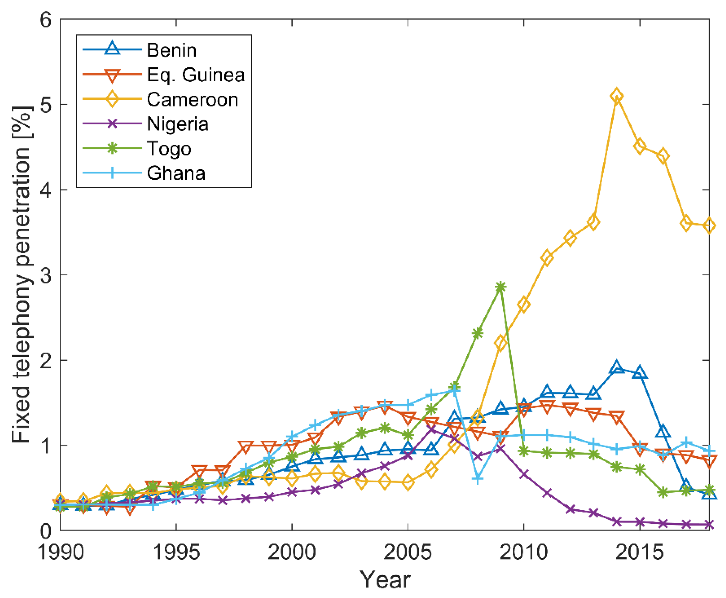
According to the World Bank report [25], fixed telephone penetration in the Gulf of Guinea peaked in the early 2010s and since then it is in constant decline. As it can be seen from Figure 1, even when it was at the highest level, the penetration reached barely 5 percent and only in one country (Cameron), while the penetration in majority of the countries in the region was less than 2%.
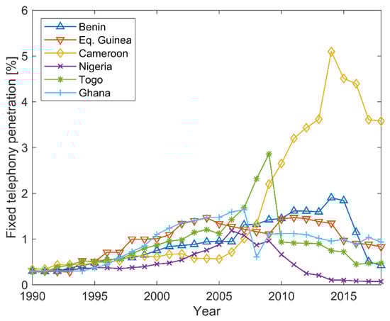
Figure 1.
Fixed telephony penetration in the Gulf of Guinea (based on data available from [25]).
From the aforementioned it is clear that fixed telephony cannot be chosen as a primary communication network for maritime sensor network in this part of the World, especially when it comes to uninhabited and inaccessible areas.
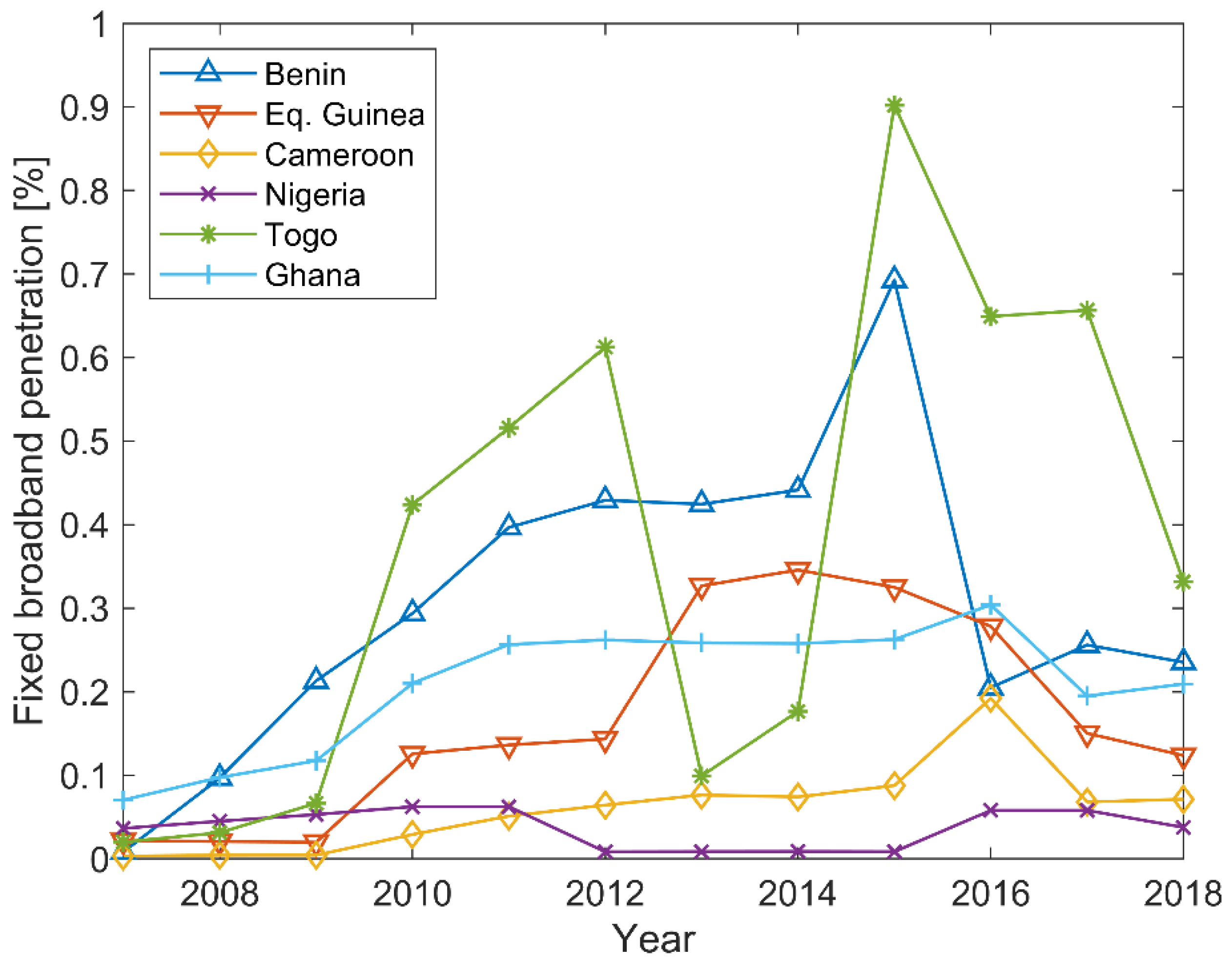
According to the same source [26], fixed broadband technologies situation is even more devastating, since penetration in all countries in the region is less than 1% (see Figure 2). One may argue that fixed broadband in the region is not generally available to the public, and that only large companies (mostly oil) possess access to fixed broadband of sufficient capacity. Although in some cases this is completely true, there are multiple reasons why company owned lines cannot be used as primary communication backbone for the maritime sensor network. The first and foremost is that in that manner the complete national maritime sensor network would be dependent on the privately owned foreign company, if indeed the company wants to grant or cede its capacities to the country. Secondly, those companies developed the network for their own purposes in the areas of interest, i.e., from the major population centers to their operations. Taking into account that HFSWRs are located away from both, it is clear why these networks cannot be used as a primary communication network for the maritime sensor network.
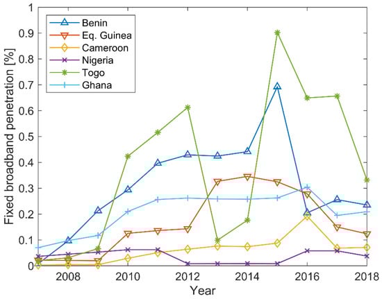
Figure 2.
Fixed Broadband penetration in the Gulf of Guinea (based on data available from [26]).
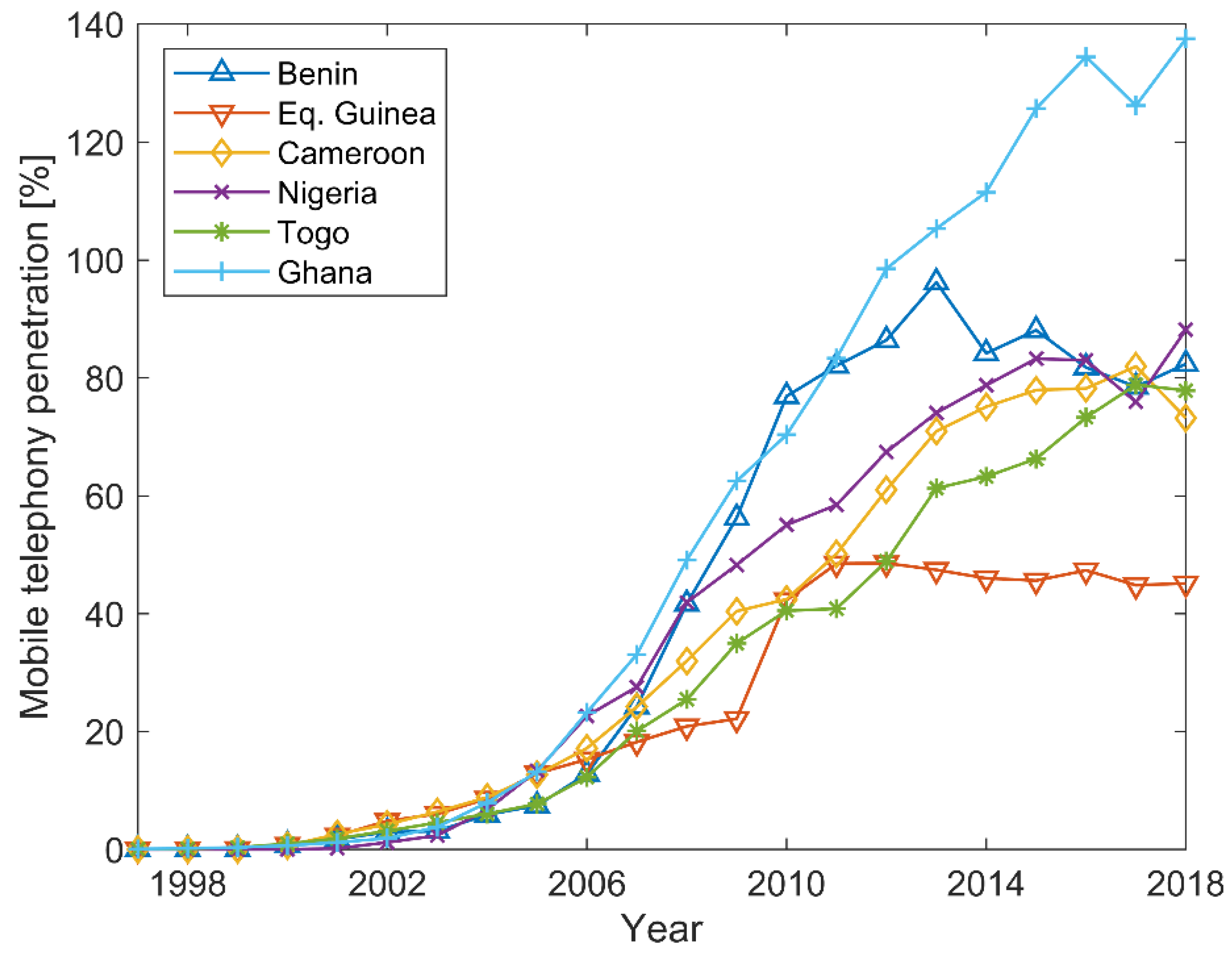
Mobile telephony might represent an optimal solution, since no additional infrastructure is needed which makes deployment costs literally negligible. Moreover, since a single HFSWR does not require high data rates (approximately 128 kb/s is quite enough) and total data-transfer is around 5 GB on a monthly basis, any currently available mobile network would be suitable as a primary communication network. Furthermore, in many countries there are state owned or controlled mobile operators, so data security should be at a very good level as well. Despite very good penetration [27], which is constantly rising (see Figure 3), mobile telephony is not available in the entire countries, especially in scarcely inhabited areas.
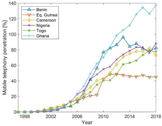
Figure 3.
Mobile telephony penetration in the Gulf of Guinea (based on data available from [27]).
In the present days, a mobile telephony network still cannot be selected as a primary communication network for the maritime sensor network in this part of the World. However, in the future, as it penetrates scarcely populated areas in the region, it may become the best option.
Communication network built with microwave (MW) links as a means of connectivity between HFSWR sites and C2s should be the most reliable and safest way. Yet, on the other hand, the costs of deployment are very high, which limits its usefulness. Taking into account that majority of the countries in the region are not in a position to further raise the maritime sensor network deployment costs, it is clear why it is not suitable here.
As the last means, there is a satellite link. The main advantages of the satellite links are increased coverage area, easy deployment and cost-effective communication solution. Although this solution may look appealing, it also has few downsides. First and foremost is the security issue, since the whole maritime sensor network is dependent on the third party (link provider). The second issue is the availability of data. HFSWR as a sensor is not very affected by meteorological factors and virtually unaffected by rain and clouds compared to the satellite links which might be very susceptible to the weather conditions. However, the IoT OTH maritime surveillance service can be designed in a way to minimize these shortcomings. The first step is measuring dependencies on meteorological factors and designing the service accordingly. The most important is to design sensor integration algorithms so the missing sensor data can be tolerated, as shown in [15]. It could be concluded that the satellite link as a means of data transfer is not a preferable solution. However, currently, in the area of the world where the system is deployed, it is the only feasible solution. This is due to the lack of other networks or lack of funds to develop a MW links network.
3. Description of the Maritime Sensor Network in the Gulf of Guinea
Full description of the observed maritime sensor network where IoT OTH maritime surveillance service is deployed can be found in [15]. In this section, only a brief description is given in order to introduce a reader with the details needed for the IoT OTH maritime surveillance service analysis, which is the paper’s main topic.
The HFSWRs are deployed at two remote locations on the coast of the Gulf of Guinea that are 100 km apart. Both locations are more than 500 km away from C2 center (central location) where the data fusion is performed. All three locations are connected via the satellite links, as shown in Figure 4, representing a generic communication architecture. The data flow for the IoT OTH maritime surveillance service starts with collecting of the raw data by the sensors at two remote locations. The initial processing of the collected data during which the detection files are created is performed on local servers, situated at remote locations. Then the implemented script on local servers starts sending the detection files to central server at Command and Control Center via satellite link using TCP protocol. The algorithm for data fusion, implemented on the central server, uses successfully transferred detection files to produce the final result in the form of accurately detected targets that are being tracked. Time, and thus transmission via the mentioned satellite link, is a key factor in successful pairing of detection files from different remote locations that should participate in the fusion process.
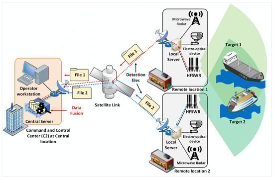
Figure 4.
Complete maritime surveillance solution architecture.
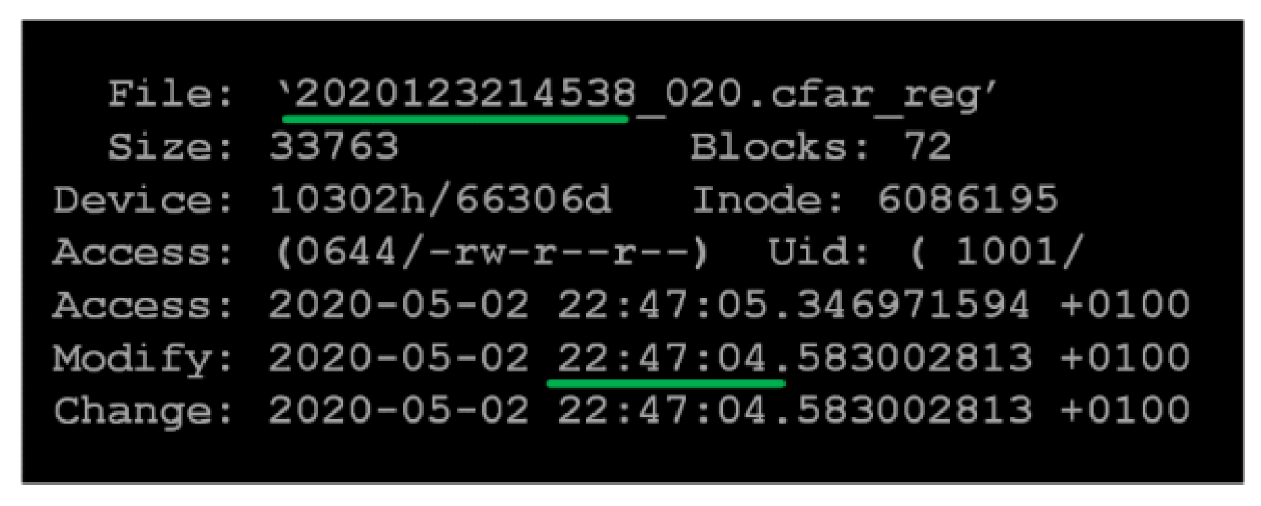
It can be seen in Figure 4 that there are other sensors in the maritime sensor network as well as HFSWRs, such as microwave radars or electro-optical devices. However, the emphasis of this paper is on the IoT OTH maritime surveillance service based on the OTH part of the maritime sensor network and HFSWRs. This is because in the given system architecture, shown in Figure 4, only HFSWRs are capable of detecting uncooperative vessels beyond the line of horizon. The detection process starts with the data collection during the so called the Coherent Integration Time (CIT). After the data are collected, they need to be processed in order to extract vessel detections. Both processes are time consuming since the first step (data collection) lasts 33 s. The time needed for the completion of the second step (collected data processing) depends on the amount of data collected during the first step. The end result is a so called cfar_reg file (detection file) which contains possible detections of the vessels in the HFSWR coverage area. Detection files are having a time stamp in their name, written in the form of yyyydddhhmmss (four digits for year, three for day of the year and two for hour, minute and second, respectively), which is actually the time when the first step (data collection and integration) started. Complete time needed for creation of the file may be seen in Figure 5.
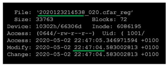
Figure 5.
Log file showing the times relevant for cfar_reg files.
The created cfar_reg file is accessed by a script for sending data. The file is sent via a satellite link as shown in Figure 4. From both remote locations, new files are sent to the central location in equal periodical intervals in order to make the vessel tracking process smooth. The client side, located at a remote location, initiates the sending of files to the server side at the central location. The server side receives the files and writes them on the disk of the central server where implemented algorithms perform target tracking and multi-sensor data fusion [14,15,16]. As it can be seen from Figure 5, data collection started at 21:45:38, while the cfar_reg file was created (modify time) at 22:47:04. One-hour difference is due to the difference between local time and UTC time used in the creation of the file name and should be neglected. The important information lies in difference between minutes and seconds. In this case it is 86.58 s, which is a time needed to completely collect, process and transmit the data at the HFSWR level. Of course, this is just an example and actual times can vary, but it provides an explanation regarding time stamps which are discussed in the following sections.
The C2 center performs fusion on HFSWR data received from both HFSWR locations. Bandwidth assigned for the HFSWR data transmission is 128 kb/s, where 64 kb/s is assigned for control commands, and the other 64 kb/s is assigned for the transmission of detection files. Naturally, the file size impacts the file transfer time. Thus, detailed distribution of the file size analyzed over the period of one year is shown in a form of histogram in Figure 6. Please note that file size depends on various factors such as density of traffic in the HFSWR coverage area, and number of false detections, which depends on weather conditions, and ionospheric interference.
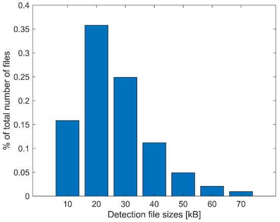
Figure 6.
Distribution of detection (cfar_reg) file sizes.
Given the distribution of the detection file sizes shown in Figure 6, the total transfer of detection file can take up to several seconds regarding that the assigned link capacity for detection file transfer is 64 kb/s. It should be noted that transfer duration is not as critical as reliability of transfer, since the lag of several seconds means nothing to the overall data fusion process at the C2 center (please see [15]). However, data missing or long lag due to the link failure or bad weather conditions may put the data fusion process in a difficult position. For this reason, TCP protocol is used for the detection file transfer, and TCP flow and error control can affect the file transfer time. In case of bad satellite link conditions frequent packet retransmissions can occur, which lead to an increase of the file transfer time. Henceforth, this paper will examine performance of the IoT OTH maritime surveillance service in various meteorological conditions. In Figure 6, it can be seen that the majority (over 80%) of the detection files are between 5 and 35 kB in size. For this reason, in the remainder of the paper we have provided the analysis for the two most frequent detection file size ranges: 15–25 kB and 25–35 kB. The conclusions derived for these two ranges apply to other detection file size ranges as well.
4. Effects of Weather Conditions in the Gulf of Guinea on the IoT Quality of Service
This section analyzes the IoT OTH maritime surveillance quality of service in meteorological conditions specific to the Gulf of Guinea. These weather conditions are:
- Clear weather, with or without light wind, both on HFSWR sites and at open sea, so called “calm sea”,
- Clear weather at HFSWR sites but with strong wind at open sea,
- Storms (heavy rain and wind) at HFSWR sites, which partially cover open sea area.
Please note: Since the IoT OTH maritime surveillance service covers an area of over 100,000 square kilometers, and with HFSWR sites nearly 100 km apart (over the airline), it is almost impossible to have identical meteorological conditions throughout that space. In practice, it often happens that a combination of the aforementioned meteorological conditions occurs.
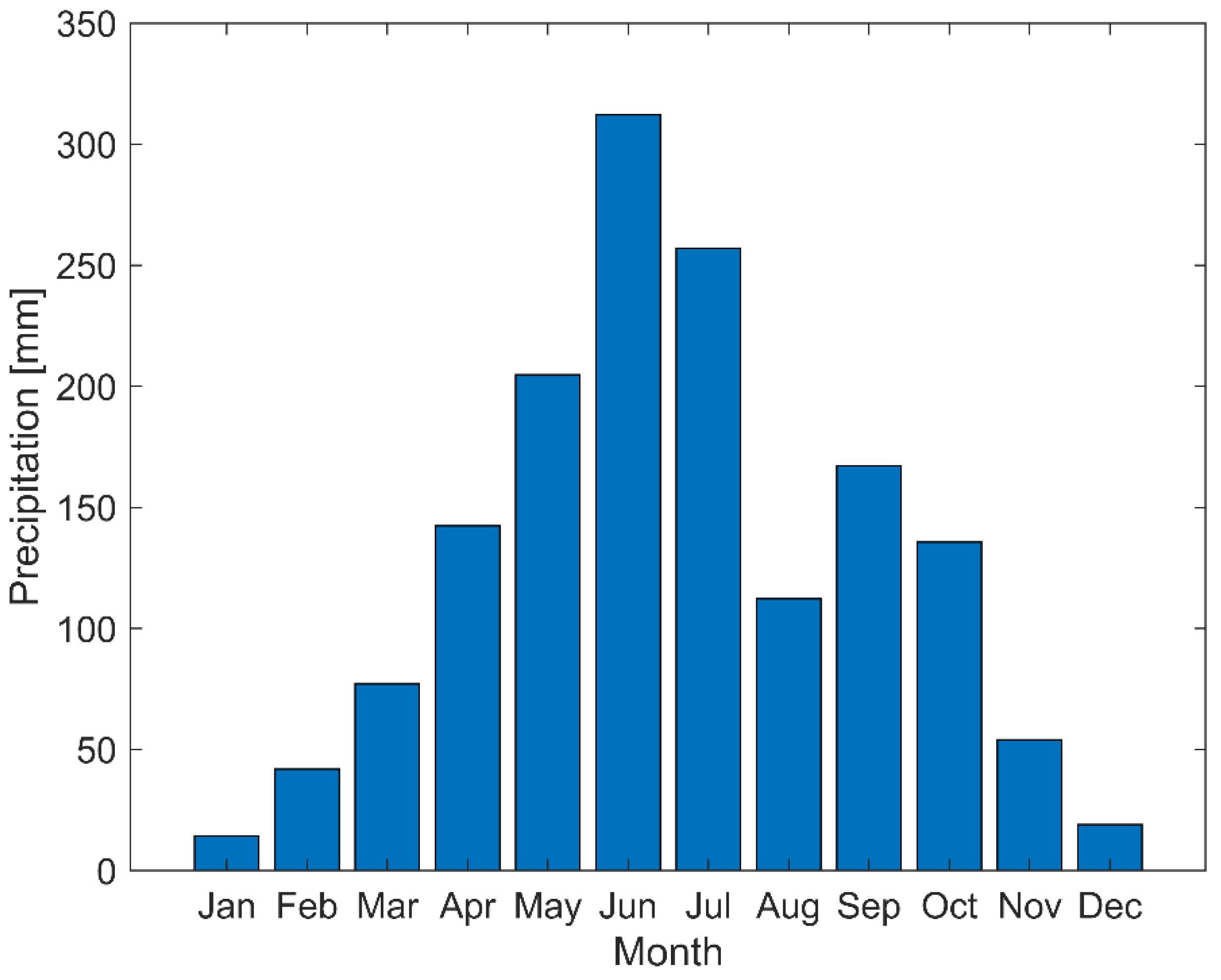
In the zone of interest there is a clear distinction between dry and rainy periods in the year. Dry season, which has its peak from December to February, is considered as a good weather period from the satellite link point of view, since rainfall is minimal and storms are quite rare. On the other hand, the period from May to July (peak of rain season) is considered as a bad weather period, since during that period rain occurs daily and violent storms are quite frequent. Figure 7 gives an overview of rain precipitation during a year in the zone of interest based on the data from the World Meteorological Organization [28]. Figure 7 shows that the period May–July is the rainiest while the period December–February is the driest.

Figure 7.
Average precipitation per months.
In the observed case, a satellite connection that operates in X band has been chosen as a backbone of the overall system, since it shows better resilience to weather conditions in general [29] than Ku or Ka bands [30]. However, since the impact of climate in the zone on the satellite link communication can be significant, this paper will examine its influence on the overall IoT OTH maritime surveillance service as well.
In the further text, three different, most common weather scenarios (atmospheric conditions) in the Gulf of Guinea that influence performances of the developed IoT OTH maritime surveillance sensor network are analyzed in detail.
4.1. Analysis during the “Calm Sea” and Calm Weather on the HFSWR Sites
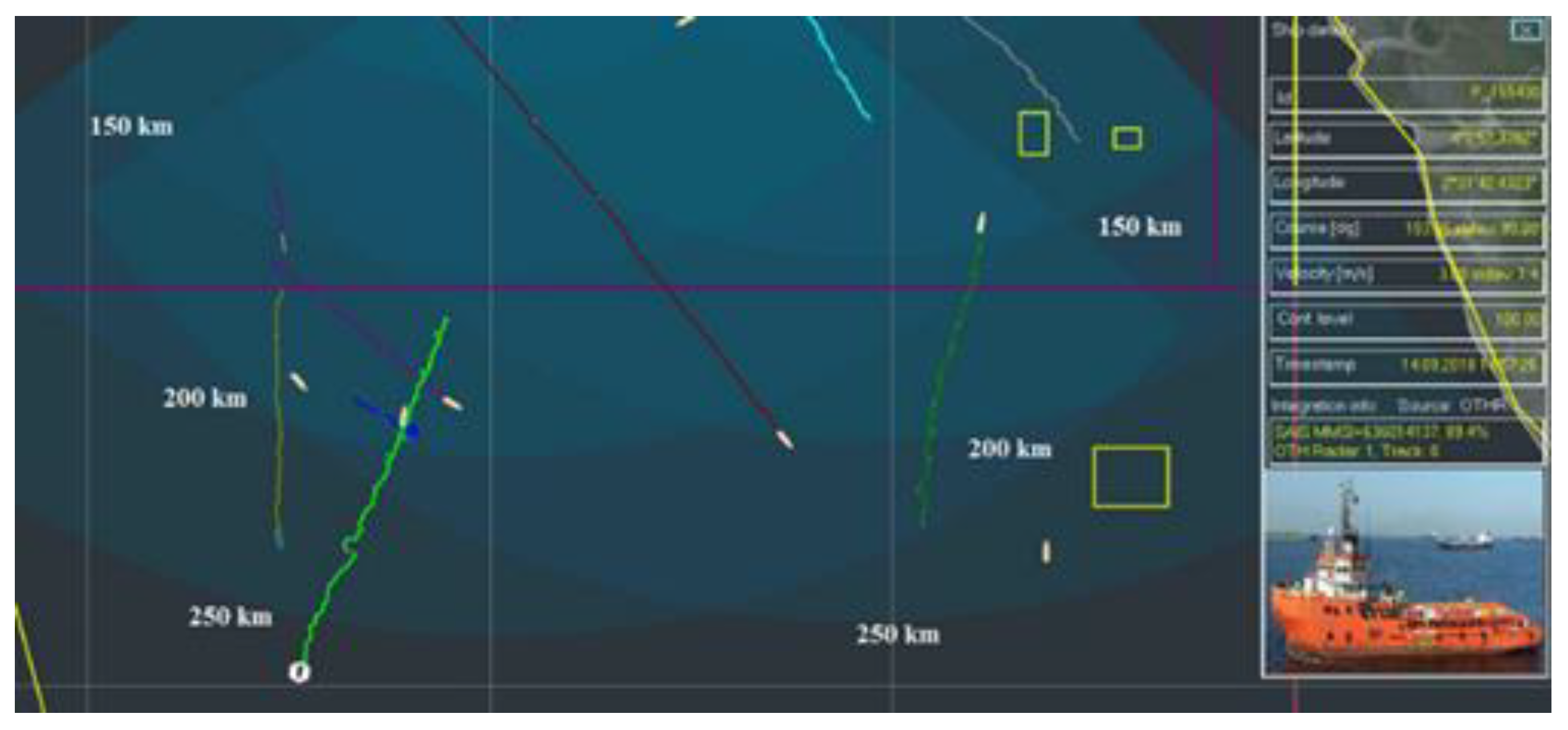
Such atmospheric conditions are characterized by clear and sunny weather with low intensity wind. The effects of such weather on the operation of HFSWRs are practically negligible. The main reason is the fact that the light wind, which characterizes such weather, has very little effect on the surface of the sea by producing waves of low altitude. Under these conditions, the sea state does not exceed 3 according to the Douglas scale [31], and according to [32], the propagation of EM waves across the sea surface is the best possible. As far as the vessel detection is concerned, it is possible even beyond the nominal HFSWR range. One such example is presented in Figure 8.
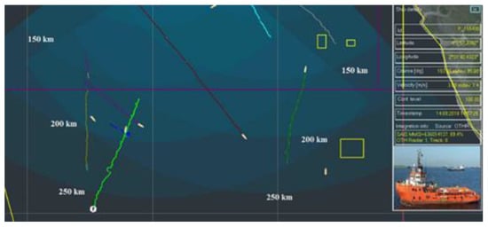
Figure 8.
Surveillance during favorable weather conditions.
In Figure 8, the vessel detection and tracking at a distance of 270 km is shown, which is well beyond the nominal HFSWR range. Furthermore, the clear weather does not introduce any difficulties in the operation of the satellite links, and there are no problems with communication between the HFSWRs and the command centers. This means that data will arrive in a timely manner and without significant delays. In clear weather there are no data delays, so it can be said that the IoT OTH maritime surveillance service operates in optimal conditions. Figure 9 shows the satellite link operation in one day by hour during a period in a day in the conditions of the “calm sea” (at the top of the Figure, we have shown the weather conditions for that day in parallel).
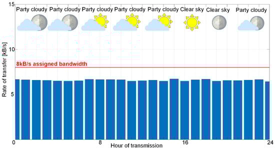
Figure 9.
Transfer rate during favorable weather conditions.
4.2. Analysis When Strong Winds Are Present in the HFSWRs Surveillance Area, but Weather on the HFSWR Site Is Calm
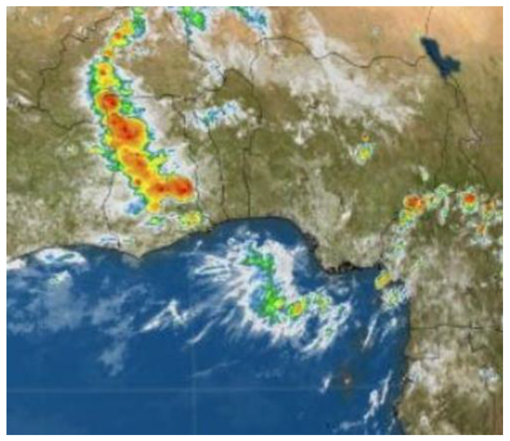
In Figure 10 a satellite image of the bad weather over one part of the IoT OTH maritime surveillance area is presented.

Figure 10.
Bad weather conditions over part of the HFSWR surveillance area.
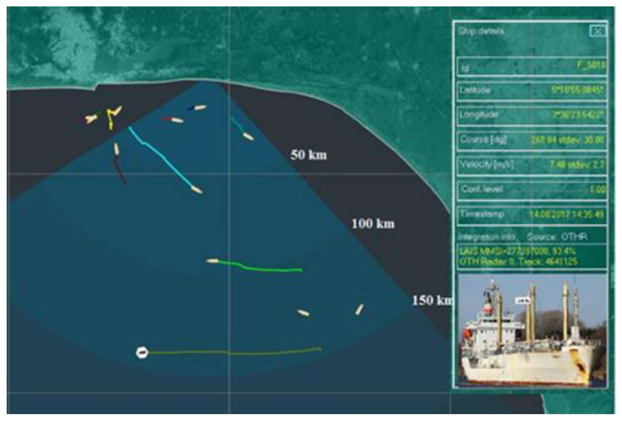
As it can be seen from Figure 10, the storm does not cover the coast itself, but “only” a large part of the HFSWR coverage area. Under these weather conditions, the range of HFSWR decreases due to the harsh surface wave propagation conditions [32]. This directly causes decline in the HFSWR vessel detection capabilities. In Figure 11 the detection capabilities of one HFSWR under the conditions described above are shown.
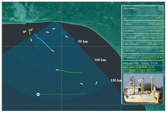
Figure 11.
HFSWR detection capabilities during bad weather conditions over part of the HFSWR surveillance.
As it can be seen in Figure 11, the range of HFSWR is practically limited to barely 150 km. On the other hand, since the weather conditions at the HFSWR sites are favorable for satellite communications, there are no significant differences in data delays in comparison to the Case A. In other words, from the satellite communication perspective this case is very similar if not identical to the previous one. Henceforth, the analysis done in the Case A is valid here as well.
4.3. Storms (Heavy Rain and Wind) at HFSWR Sites Which Partially Cover the Observation Area
In Figure 12 a satellite image of the bad weather conditions over the HFSWR sites which partially extended to the surveillance area is shown.
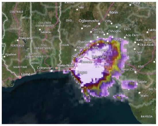
Figure 12.
Bad weather conditions over the HFSWR sites.
From Figure 12 it can be seen that the storm has hit the coast where HFSWRs were installed, but the majority of the HFSWR surveillance area has not been affected. Even in these weather conditions, the range of HFSWRs will decrease due to harsh surface wave propagation conditions. Yet, this decrease is not as drastic as that in the previous example, since the furthest target is detected at the distance of about 180 km (Figure 13).
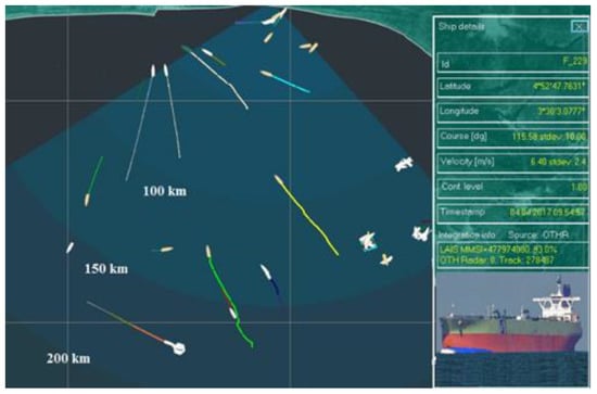
Figure 13.
HFSWR detection capabilities during bad weather conditions over part of the HFSWR surveillance area and HFSWR sites.
It should be emphasized here that detection files from HFSWRs are not received at regular intervals, as the satellite communication is very difficult, due to heavy rain. In the event of severe weather conditions over the HFSWR sites, there are occasional interruptions in the satellite communication.
Therefore, data delays occur and algorithms for multi-sensor data fusion must perform HFSWR tracks predictions and maintain tracks based on them. Despite all this, in Figure 13 it can be seen that the algorithms manage to keep the traces stable, thus providing the full information to the end user. However, this will not be possible without thorough statistical analyses of the IoT OTH maritime surveillance service, which is presented in the following section.
Figure 14 shows the satellite link operation in one day by hour during a period in a day in the conditions of the storms (at the top of the Figure, we have shown the weather conditions for that day in parallel).
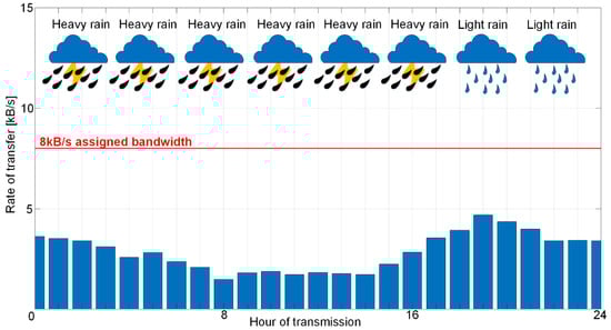
Figure 14.
Transfer rate during bad weather conditions.
Drop in the transfer rate is obvious in comparison to Figure 9 during favorable weather conditions of about 40–50%.
The analysis given in this section shows that weather conditions over the surveilled maritime area and over the HFSWR sites have impact on the IoT OTH maritime surveillance service, but the impact type differs. Weather conditions over the surveilled maritime area impact on the range that HFSWRs cover. Weather conditions also impact the quality of the content in the detection files which then impacts the fusion algorithms effort to provide the high-quality results to the end users. On the other hand, weather conditions over the HFSWR sites impact on the transmission of the detection files to C2 center. In case of severe weather conditions, even temporary outages of the satellite link may occur, which can lead to problems in providing the relevant information about the surveilled maritime area to the end users.
5. Statistical Analysis of Quality of IoT Service during the Year
In this section a statistical analysis of the quality of the IoT OTH maritime surveillance service over a good weather (dry season which has its peak from December to February) and bad weather period (from May to July, peak of rain season) will be presented. Note that the major impact on the IoT OTH maritime surveillance service is the satellite communication that represents the communication backbone of the overall maritime surveillance sensor network depicted in Figure 4. In Section 3 we have explained in detail how detection files are generated and distribution of detection file sizes is presented (Figure 6).
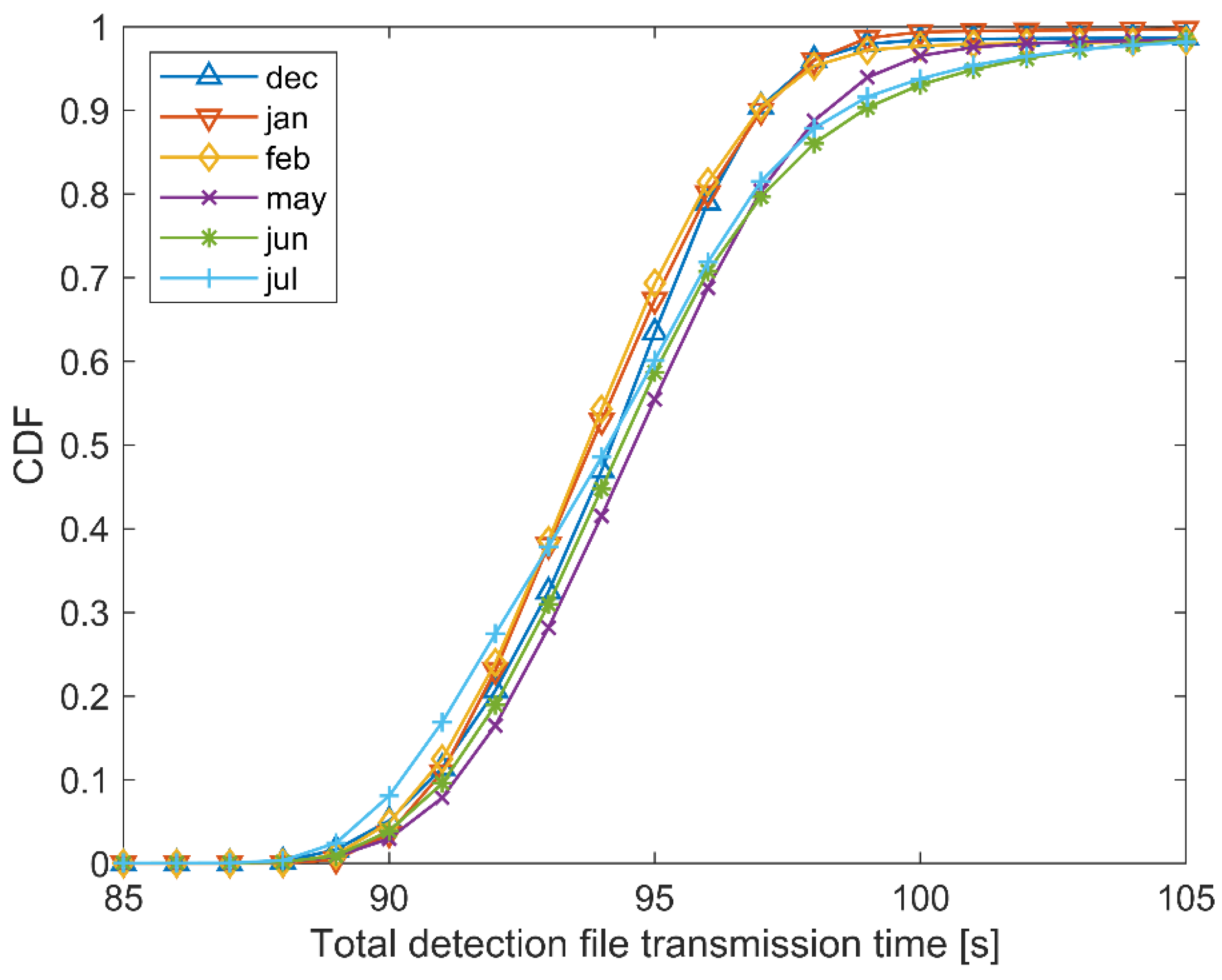
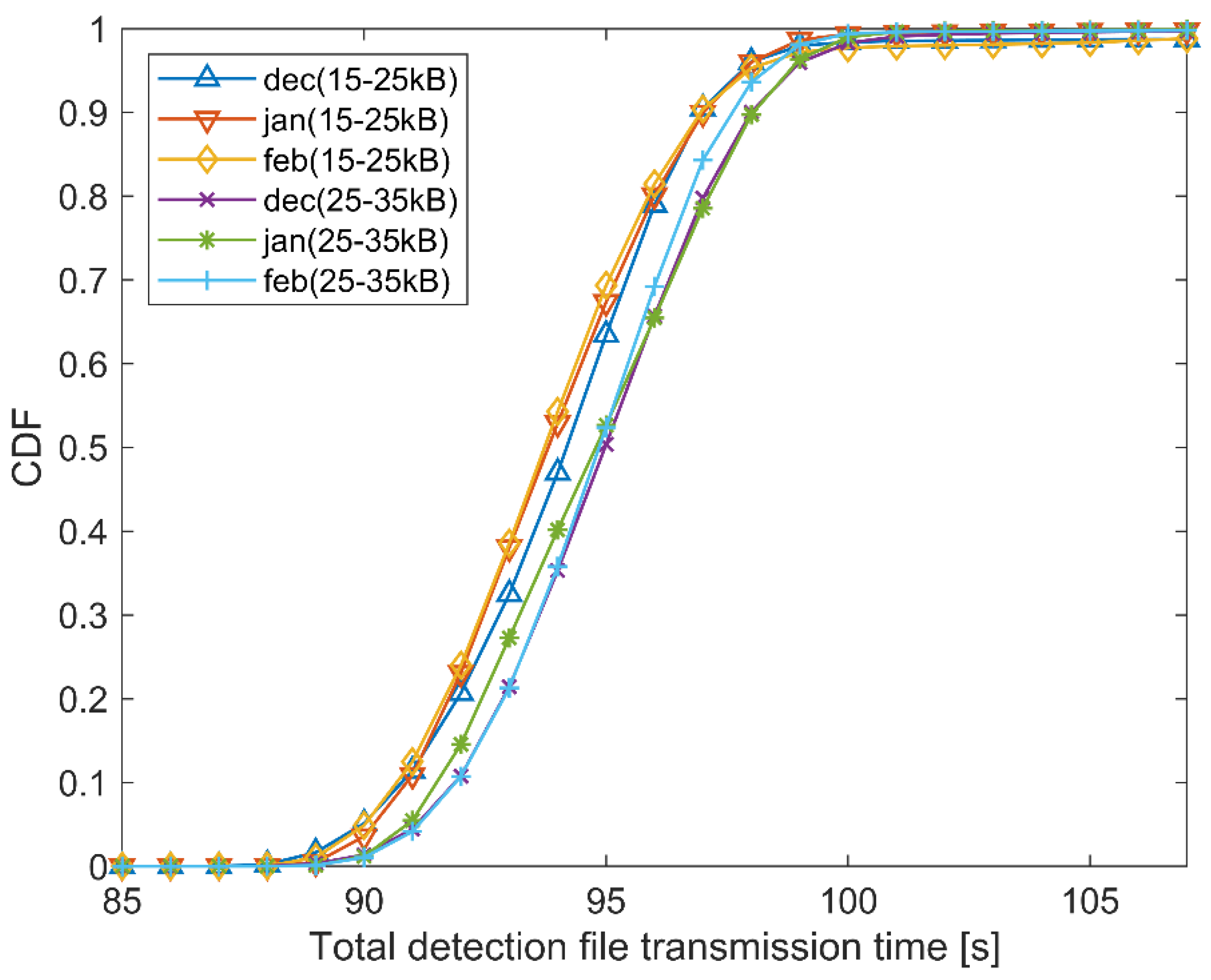
In Figure 15 and Figure 16, we have shown the cumulative distribution function (CDF) of the time frame that is measured from the data collection start at the HFSWR location to the end of the detection file transfer to central location (referred as total detection file transmission time in the remainder of this section). Given the distribution of the detection file sizes shown in Figure 6, we have shown the cumulative distribution of total detection file transmission time for the two most common file size ranges.
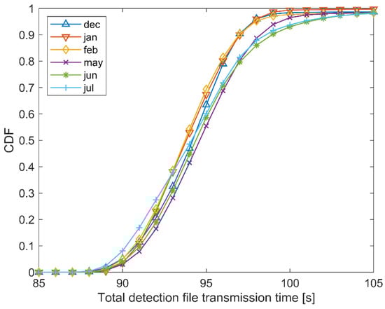
Figure 15.
CDF for detection file size range 15–25 kB.
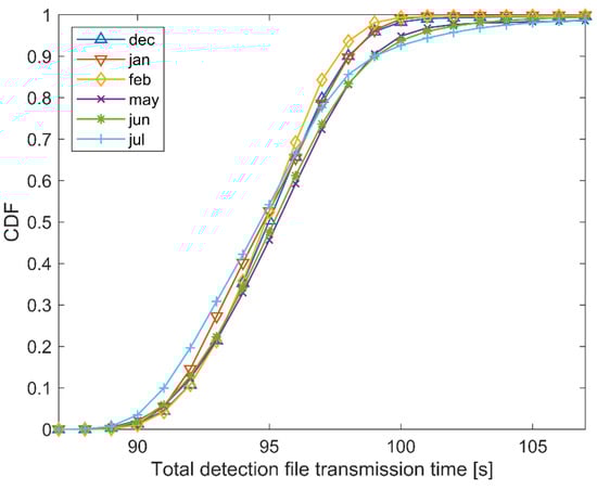
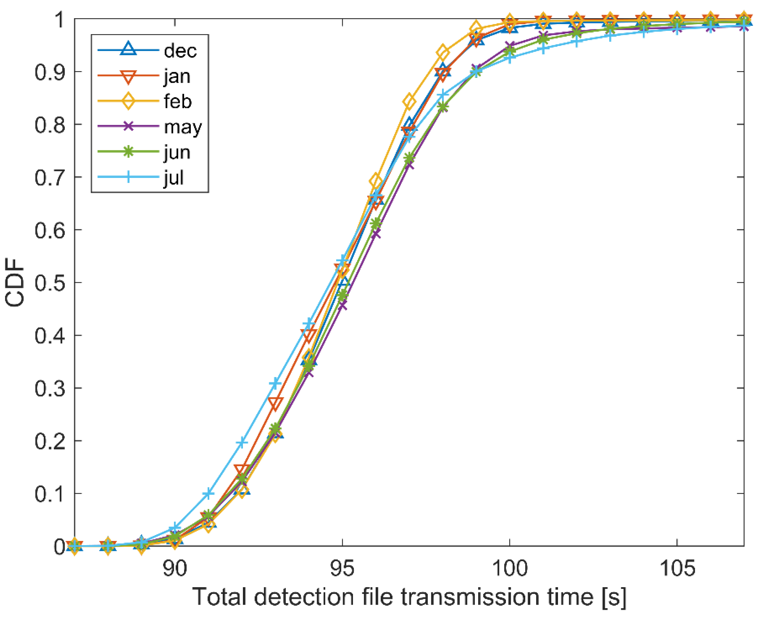
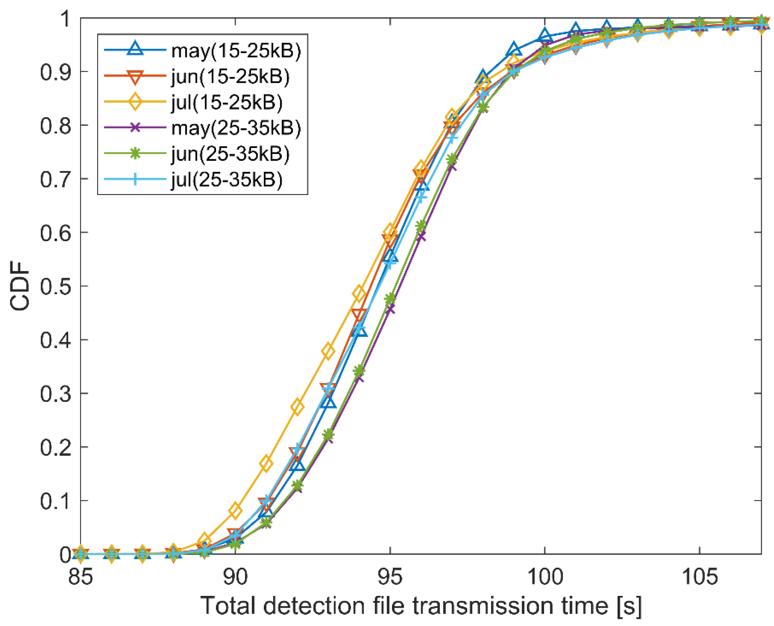
Figure 16.
CDF for detection file size range 25–35 kB.
Figure 15 shows the cumulative distribution for the 15–25 kB range, while Figure 16 shows the cumulative distribution for the 25–35 kB range. Figure 15 and Figure 16 show the three rainiest months (May–July) and the three driest months (December–February), with the idea to observe whether there are some differences in the total detection file transmission times. The CDF of the rainiest months reaches the value 1 later than the CDF of the driest months. This means that, on average, it takes more time to transfer files to the central location when the weather conditions have more negative impact on the satellite link. However, given that the overall system is robust and can tolerate differences up to several seconds, the given differences in total detection file transmission times between the worst and the best weather condition months are acceptable.
Figure 17 and Figure 18 show the comparison of total detection file transmission time CDF for the two most common file size ranges—15–25 kB and 25–35 kB for the driest and rainiest months, respectively. As expected, the file size does have an impact on the total detection file transmission time as the CDF for range 25–35 kB reaches value 1 later than the CDF for range 15–25 kB. However, the time differences are not significant and do not affect the overall IoT OTH maritime surveillance service performance.
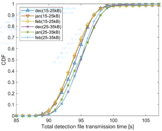
Figure 17.
CDF of 15–25 kB and 25–35 kB for Dec–Feb.

Figure 18.
CDF of 15–25 kB and 25–35 kB for May–July.
In order to properly estimate the service performance parameters, it is needed to analyze service behavior on a monthly basis and to derive a mathematical model of that behavior. It is important to emphasize that neither of the derived distributions describes empirical data perfectly. However, similarity of the derived distributions and empirical data is very high so it might be said that the derived distributions are properly describing the empirical data. Since those analyses may prove to be too lengthy, only the best and the worst matching will be presented and discussed further. The conclusions are valid for the whole observed time frame.
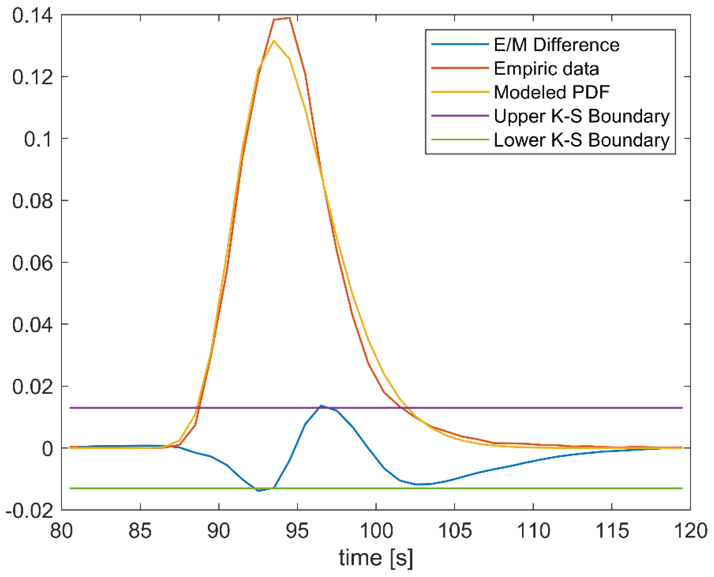
Firstly, the best matching case (June 2018) is presented (matching with 20 different probability density functions (PDF) is tested). After analysis in Matlab software package [33] is done, it has been found that the best mathematical description for the data collected during June 2018 can be achieved with PDF called “generalized extreme value” [34]. Equation (1) is a mathematical formulation of the aforementioned PDF, while the comparison of modeled PDF and empirical data is shown in Figure 19.
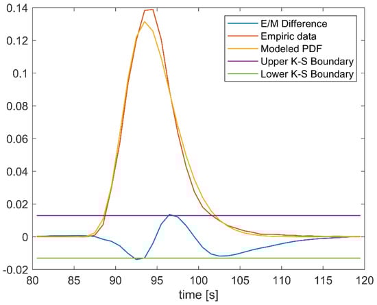
Figure 19.
Statistical modeling for June 2018.
Please note that:
Parameters needed to achieve a desired PDF are:
- k = −0.095368,
- σ = 2.8064,
- µ = 13.3195.
As it can be seen from Figure 19 there are some differences between the empirical data and modeled PDF, which are presented with red and orange lines, respectively. These differences cause that difference in CDFs of empirical and modeled data (blue line, denoted with Empiric/Modeled (E/M) Difference) goes over the boundaries set by the Kolmogorov–Smirnoff (K-S) test (purple and green lines, denoted with the Upper K-S Boundary and Lower K-S Boundary). However, although some irregularities exist, it may still be said that the modeled PDF can be used to describe behavior of the empirical data with a good accuracy, because K-S boundary is violated for only ~5% of samples with the maximum violation of ~6%.
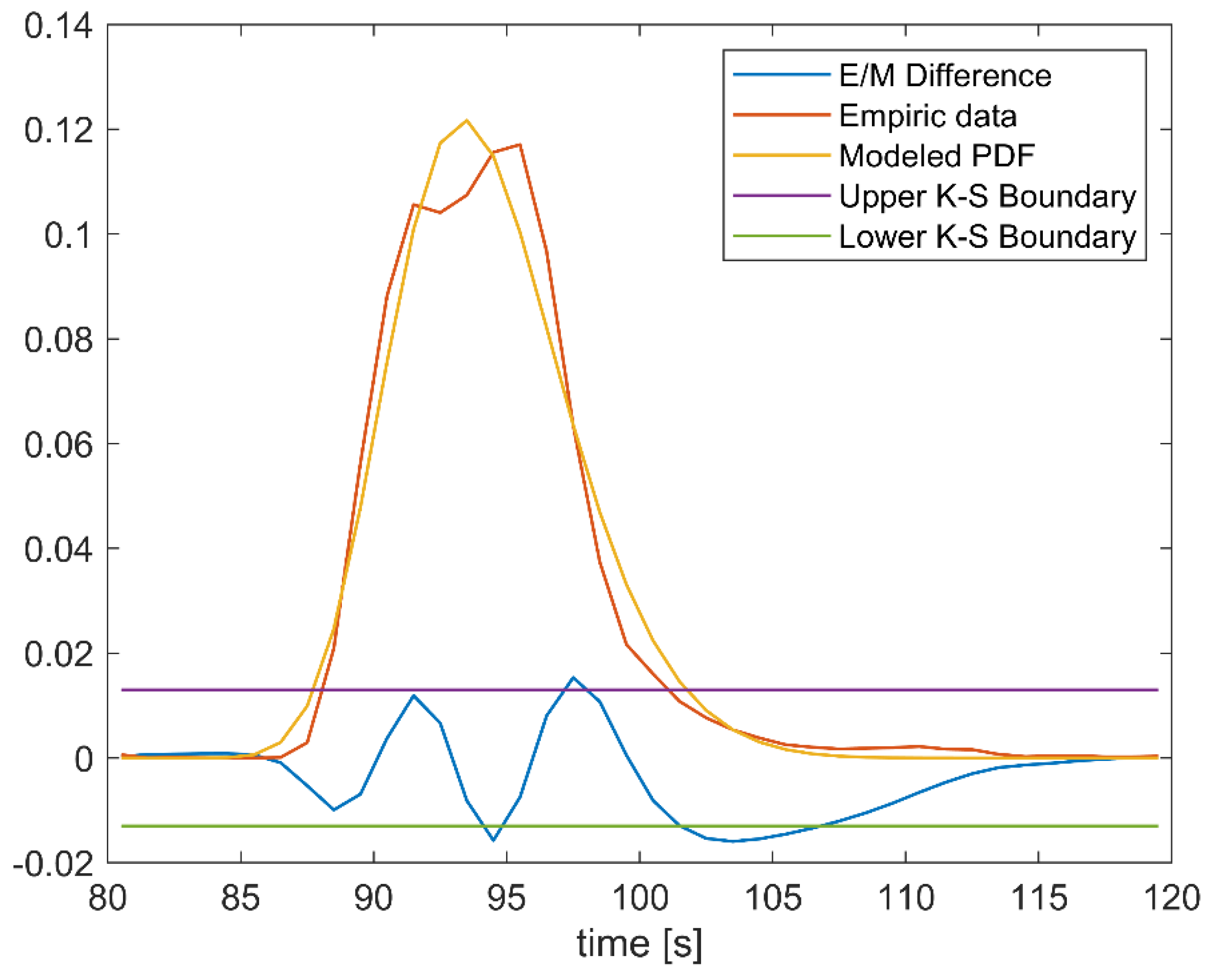
Next, the worst matching case (July 2018) is presented. Matlab software package is once again used for the analysis and it is concluded that generalized extreme value PDF again gives the best results. Naturally, the parameters are different and they are:
- k = −0.13687,
- σ = 3.0326,
- µ = 12.9111.
Comparison of the modeled and empirical data is shown in Figure 20.
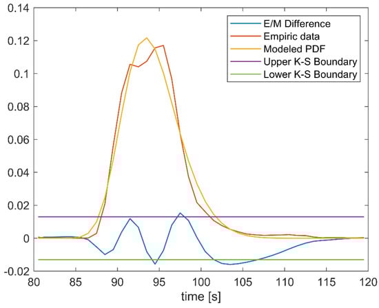
Figure 20.
Statistical modeling for July 2018.
From Figure 20 it can be seen that the differences between the modeled and empirical data are greater than in the previous case. This is easily observed either by comparing PDFs or the differences between CDFs, which consequently goes over the Kolmogorov–Smirnoff test boundaries on multiple occasions. However, of all the tested PDFs the one presented here gives the best results (K-S boundary is violated for ~15% of samples with the maximum violation of ~20%) and it is taken as a mathematical model of the empirical data.
Based on the presented analysis it may be said that modeled PDFs can be reliably used to describe and predict the IoT OTH maritime surveillance service behavior. This can be further used in order to increase the data fusion process stability and thus reliability of the IoT OTH maritime surveillance service as a whole.
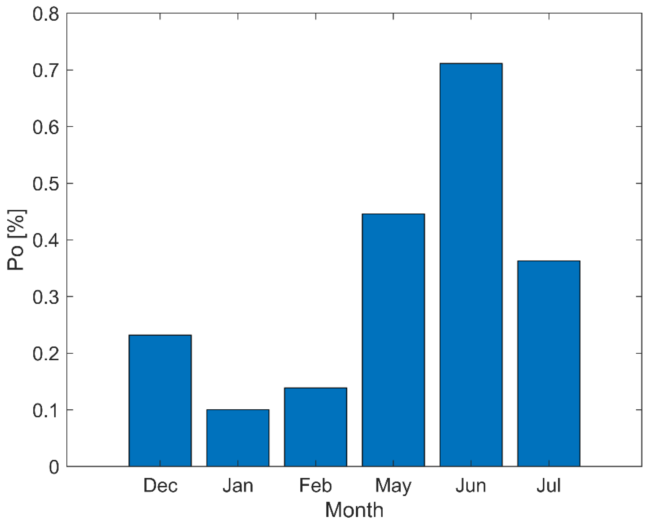
During the harsh weather conditions, the satellite link can perform poorly, and numerous packet retransmissions might occur and TCP connection might be disrupted. In case when the detection file is not transmitted timely to the central location this can lead to dropping the detection file at the radar location. This is due to the detection file no longer being relevant and thus not being eligible for use in the data fusion process at the C2 center. For that reason, we have observed the outage probability using the following definition: Po = Nt/Ntot, where Po is the outage probability, Nt is the number of unsuccessfully (not on time) delivered detection files to C2 center, and Ntot is the total number of generated detection files at the radar location.
In Figure 21 the outage probabilities are shown for the three rainiest and the three driest months as we expect that the rainier months should have a greater outage probability. Figure 21 shows that the rainier months indeed have a greater outage probability which comes from worse weather conditions on average (Po: 0.1–0.25% in good weather conditions, 0.35–0.7% in bad weather conditions).
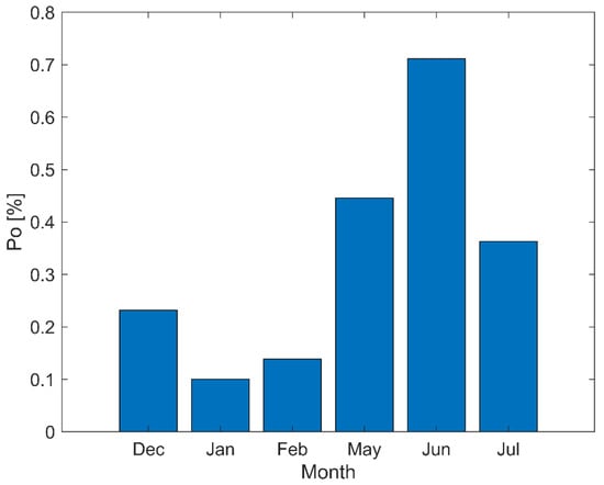
Figure 21.
Outage probability comparison between rainiest and driest months.
In this section, we have derived the IoT OTH maritime surveillance service performance dependency on weather conditions, as a function of data latency. From the presented analyses it is clear that the average data latency is about 90 s, while the outliers can be as high as 120 s. This was a key information during design of data fusion algorithms presented in [14,15,16], where a critical latency for the whole end to end process, starting from the raw data collection and ending with the data display to the end user, is set to 250 s. The analyses shown in Figure 15, Figure 16, Figure 17, Figure 18, Figure 19 and Figure 20 show that this requirement is always satisfied, and that the IoT OTH maritime surveillance service operates stably in all weather conditions specific for the Gulf of Guinea. The other key information (from data fusion point of view) these analyses provide is the outage probability, presented in Figure 21. It can be seen that a high variance of outage occurrence can be expected, which requires additional mechanisms in data fusion algorithms in order to maintain stable tracking. Presented analyses undoubtedly show that the transmission via the satellite link is the optimal solution for the IoT OTH maritime surveillance service in the observed environment.
6. Conclusions
In this paper the challenges and constraints when over the horizon (OTH) maritime surveillance service is built on an Internet of Things (IoT) as its backbone are examined. The service utilizes High Frequency Surface Wave Radars (HFSWRs) as primary sensors and relies on a satellite communication network as its communication infrastructure in a harsh environment. The whole IoT OTH maritime surveillance network is deployed in the Gulf of Guinea and it entered operational service. The performance analysis encloses multiple steps starting with the raw data gathering from the open sea. It continues with the data processing by HFSWRs at the remote sites and ends with the data transferring to the server on a C2 location, via the satellite network.
Thorough statistical analysis has been conducted during the extreme periods (the driest and rainiest months) in order to mathematically describe the IoT service behavior as precisely as possible. The mathematical model of the IoT OTH maritime surveillance service behavior is verified with the Kolmogorov–Smirnoff test. It should be noted that during this analysis each empirical data set is tested with nearly 20 different PDFs. Analyses presented in the paper show that average service latency is about 90 s, but it can rise to about 120 s, which is used as a key information during the sensor data fusion algorithm design. Validity of the analyses is demonstrated through high quality of service with an outage probability of just 0.1% in the driest months up to the 0.7% in the rainiest months. According to the analysis presented in this paper it is shown that the IoT OTH maritime surveillance service based on HFSWRs which relies on the satellite communication infrastructure can be a viable and reliable solution in the areas defined by harsh meteorological conditions. Moreover, the IoT service behavior can be predicted very well by the statistical models presented in this paper. At the end, the work presented here may be used as a guideline for deployment of other maritime surveillance service solutions in other equatorial regions.
For the future work we intend to expand the sensor network and gather new data in order to further improve the statistical description of the IoT OTH maritime surveillance service behavior.
Author Contributions
Conceptualization, R.P. and D.N.; methodology, D.S.; software, M.N.; validation, D.S. and Z.C.; formal analysis, R.P. and D.D.; investigation, R.P.; resources, R.P.; data curation, M.N.; writing—original draft preparation, R.P. and D.S.; writing—review and editing, Z.C., D.D. and D.N.; visualization, Z.C.; supervision, D.S.; project administration, R.P.; funding acquisition, R.P. All authors have read and agreed to the published version of the manuscript.
Funding
The research is funded by the Vlatacom Institute of High Technologies under project #89.1. The APC is also covered by Vlatacom Institute of High Technologies.
Acknowledgments
Authors of the paper would like to thank to Ivan Gluvacevic for his help.
Conflicts of Interest
The authors declare no conflict of interest.
References
- Global Report on Maritime Piracy; United Nations Institute for Training and Research (UNITAR): Geneva, Switzerland, 2014; Available online: https://www.unitar.org/learning-solutions/publications/unosat-global-report-maritime-piracy-geospatial-analysis-1995-2013 (accessed on 10 February 2021).
- UN News. UN Security Council Urges “Comprehensive Response” to Piracy off Somali Coast. 7 November 2017. Available online: https://news.un.org/en/story/2017/11/570172-un-security-council-urges-comprehensive-response-piracy-somali-coast (accessed on 10 February 2021).
- European Union. European Union Naval Force ATALANTA, EU. Available online: https://eunavfor.eu/mission/ (accessed on 14 February 2021).
- Starr, S. Maritime Piracy on the Rise in West Africa. CTC Sentin. 2014, 7, 22–26. [Google Scholar]
- World Economic Forum. Available online: https://www.weforum.org/agenda/2019/06/west-africa-is-becoming-the-world-s-piracy-capital-here-s-how-to-tackle-the-problem/ (accessed on 14 February 2021).
- The United Nations Office on Drugs and Crime. May 2019. Available online: https://www.unodc.org/nigeria/en/press/west-africa-loses-2-3-billion-to-maritime-crime-in-three-years-as-nigeria--unodc-rally-multi-national-efforts-to-thwart-piracy-in-the-gulf-of-guinea.html (accessed on 14 February 2021).
- Helzel, T.; Kniephoff, M.; Petersen, L. Oceanography radar system WERA: Features, accuracy, reliability and limitations. Turk. J. Elec. Eng. Comp. Sci. 2010, 18, 389–397. [Google Scholar]
- Shay, L.K.; Martinez-Pedraja, J.; Cook, T.M.; Haus, B.K.; Weisberg, R.H. High-Frequency Radar Mapping of Surface Currents Using WERA. J. Atmos. Ocean. Technol. 2007, 24, 484–503. [Google Scholar] [CrossRef]
- Liu, Y.; Weisberg, R.H.; Merz, C. Assessment of CODAR SeaSonde and WERA HF Radars in Mapping Surface Currents on the West Florida Shelf. J. Atmos. Ocean. Technol. 2014, 31, 1363–1382. [Google Scholar] [CrossRef]
- Lipa, B.; Barrick, D.; Alonso-Martirena, A.; Fernandes, M.; Ferrer, M.I.; Nyden, B. Brahan Project High Frequency Radar Ocean Measurements: Currents, Winds, Waves and Their Interactions. Remote Sens. 2014, 6, 12094–12117. [Google Scholar] [CrossRef] [Green Version]
- Sun, W.; Ji, M.; Huang, W.; Ji, Y.; Dai, Y. Vessel Tracking Using Bistatic Compact HFSWR. Remote Sens. 2020, 12, 1266. [Google Scholar] [CrossRef] [Green Version]
- Sevgi, L.; Ponsford, A.; Chan, H.C. An integrated maritime surveillance system based on high-frequency surface-wave radars. Part 1. Theoretical background and numerical simulations. IEEE Antennas Propag. Mag. 2001, 43, 28–43. [Google Scholar] [CrossRef]
- Ponsford, A.; Sevgi, L.; Chan, H.C. An integrated maritime surveillance system based on high-frequency surface-wave radars. Part 2. Operational status and system performance. IEEE Antennas Propag. Mag. 2001, 43, 52–63. [Google Scholar] [CrossRef]
- Stojkovic, N.; Nikolic, D.; Puzovic, S. Density Based Clustering Data Association Procedure for Real–Time HFSWRs Tracking at OTH Distances. IEEE Access 2020, 8, 39907–39919. [Google Scholar] [CrossRef]
- Nikolic, D.; Stojkovic, N.; Popovic, Z.; Tosic, N.; Lekic, N.; Stankovic, Z.; Doncov, N. Maritime over the horizon sensor inte-gration: HFSWR data fusion algorithm. Remote Sens. 2019, 11, 852. [Google Scholar] [CrossRef] [Green Version]
- Nikolic, D.; Stojkovic, N.; Lekic, N. Maritime over the Horizon Sensor Integration: High Frequency Surface-Wave-Radar and Automatic Identification System Data Integration Algorithm. Sensors 2018, 18, 1147. [Google Scholar] [CrossRef] [PubMed] [Green Version]
- Chiani, M.; Giorgetti, A.; Paolini, E. Sensor Radar for Object Tracking. Proc. IEEE 2018, 106, 1022–1041. [Google Scholar] [CrossRef] [Green Version]
- vOTHR. Available online: https://www.vlatacominstitute.com/over-the-horizon-radar (accessed on 15 April 2021).
- Nikolic, D.; Stojkovic, N.; Petrovic, P.; Tosic, N.; Lekic, N.; Stankovic, Z.; Doncov, N. The high frequency surface wave radar solution for vessel tracking beyond the horizon. Facta Univ. Ser. Electron. Energetics 2020, 33, 37–59. [Google Scholar] [CrossRef] [Green Version]
- ITU-D: ICT Data and Statistics (IDS). Available online: https://www.itu.int/ITU-D/ict/statistics/ict/ (accessed on 15 April 2021).
- World Bank Open Data. Available online: https://data.worldbank.org/ (accessed on 17 April 2021).
- Peel, M.C.; Finlayson, B.L.; McMahon, T.A. Updated world map of the Köppen-Geiger climate classification. Hydrol. Earth Syst. Sci. 2007, 11, 1633–1644. [Google Scholar] [CrossRef] [Green Version]
- Christian, H.J.; Blakeslee, R.; Boccippio, D.J.; Boeck, W.L.; Buechler, D.E.; Driscoll, K.T.; Goodman, S.J.; Hall, J.M.; Koshak, W.J.; Mach, D.M.; et al. Global frequency and distribution of lightning as observed from space by the Optical Transient Detector. J. Geophys. Res. Space Phys. 2003, 108, ACL 4-1–ACL 4-15. [Google Scholar] [CrossRef]
- Petrovic, R.; Simic, D.; Drajic, D.; Cica, Z.; Nikolic, D.; Peric, M. Designing Laboratory for IoT Communication Infrastructure Environment for Remote Maritime Surveillance in Equatorial Areas Based on the Gulf of Guinea Field Experiences. Sensors 2020, 20, 1349. [Google Scholar] [CrossRef] [PubMed] [Green Version]
- Fixed Telephone Subscriptions (per 100 People). Available online: https://data.worldbank.org/indicator/IT.MLT.MAIN.P2?view=map (accessed on 15 April 2021).
- Fixed Broadband Subscriptions (per 100 People). Available online: https://data.worldbank.org/indicator/IT.NET.BBND.P2 (accessed on 15 April 2021).
- Mobile Cellular Subscriptions (per 100 People). Available online: https://data.worldbank.org/indicator/IT.CEL.SETS.P2 (accessed on 15 April 2021).
- World Weather Information Service. Available online: https://worldweather.wmo.int/ (accessed on 15 April 2021).
- Scaramuzza, P.; Rubino, C.; Caruso, M.; Tiebout, M.; Bevilacqua, A.; Neviani, A. Class-J SiGe X -Band Power Amplifier Using a Ladder Filter-Based AM–PM Distortion Reduction Technique. IEEE Trans. Circuits Syst. I Regul. Pap. 2018, 65, 3780–3789. [Google Scholar] [CrossRef]
- Yeo, J.X.; Lee, Y.H.; Ong, J.T. Rain Attenuation Prediction Model for Satellite Communications in Tropical Regions. IEEE Trans. Antennas Propag. 2014, 62, 5775–5781. [Google Scholar] [CrossRef]
- NOAA. Table 3700: Sea State. Available online: https://www.nodc.noaa.gov/woce/woce_v3/wocedata_1/woce-uot/document/wmocode.htm (accessed on 15 April 2021).
- International Telecommunication Union. Reccommendation ITU-R P.368-9 Ground-Wave Propagation Curves for Frequencies between 10 KHz and 30 MHz; ITU-R: Geneva, Switzerland, 2007. [Google Scholar]
- Matlab—MathWorks. Available online: https://www.mathworks.com/products/matlab.html (accessed on 14 February 2021).
- Papoulis, A.; Pillai, S.U. Probability, Random Variables and Stochastic Processes, 4th ed.; McGraw-Hill: New York, NY, USA, 2002. [Google Scholar]


Publisher’s Note: MDPI stays neutral with regard to jurisdictional claims in published maps and institutional affiliations. |
© 2021 by the authors. Licensee MDPI, Basel, Switzerland. This article is an open access article distributed under the terms and conditions of the Creative Commons Attribution (CC BY) license (https://creativecommons.org/licenses/by/4.0/).