Abstract
The design of a solar PV system and its performance evaluation is an important aspect before going for a mass-scale installation and integration with the grid. The parameter evaluation of a solar PV model helps in accurate modeling and consequently efficient designing of the system. The parameters appear in the mathematical equations of the solar PV cell. A Chaos Induced Coyote Algorithm (CICA) to obtain the parameters in a single, double, and three diode model of a mono-crystalline, polycrystalline, and a thin-film solar PV cell has been proposed in this work. The Chaos Induced Coyote Algorithm for extracting the parameters incorporates the advantages of the conventional Coyote Algorithm by employing only two control parameters, making it easier to include the unique strategy that balances the exploration and exploitation in the search space. A comparison of the Chaos Induced Coyote Algorithm with some recently proposed solar photovoltaic cell parameter extraction algorithms has been presented. Analysis shows superior curve fitting and lesser Root Mean Square Error with the Chaos Induced Coyote Algorithm compared to other algorithms in a practical solar photovoltaic cell.
1. Introduction
Renewable energy, particularly from the sun, has increased in usage due to the increasing population, ever-growing industrial needs, depletion of fossil fuel reserves, and many environmental problems [1,2]. Solar energy does not cause any kind of pollution, i.e., it is a clean form of energy, it can also be readily available at a properly chosen site [3].
The complexity and non-linearity of the solar cell equations, in addition to various instability problems, act as a hurdle to the PV system [4,5,6,7]. Several other reasons, including temperature, solar radiation, cable losses, dust accumulation, soiling, and shading, also affect I–V characteristics [8,9]. Hence, to evaluate the solar PV system’s performance in actual working conditions, a thorough analysis of the solar PV system is essential. While it may not be possible to practically study these effects, as physical factors change rapidly, an accurate model of the solar PV system will give a close idea of the requirements of the practical implementation [10]. Thus, it becomes necessary to develop accurate models for it. The literature proposes different models to represent a solar cell differently from each other by the number of diodes they incorporate. The single diode models (SDM) and the double diode models (DDM) are the more famous models [11,12]. The models represent the current-voltage characteristics (I–V), but only for domestic purposes. Hence a three diode model (TDM) [12] was developed, which can also be used for industrial applications [13]. With the change in the number of diodes in the solar cell’s equivalent circuits, there is also a change in the number of extracted parameters. Although the single-diode model is accurate, the saturation current of the solar PV cell varies linearly with charge diffusion and recombination in the space charge layer [14], and thus more accurate representation is possible by adding two diodes in parallel to the ideal current source and associated series and shunt resistors [15]. DDM is more relevant for the operation of PV cells at low irradiance [14]. In order to include the effect of current due to the leakage through the peripheries, a third diode can be included in parallel [16].
To achieve the characteristics of the actual PV system, the simulation model must provide accurate parameter estimation, i.e., an optimized parameter estimation technique is required. There are many techniques available that can be used to optimize the values of these parameters. The various techniques include the classical techniques (analytical and numerical methods), as shown in Table 1, and stochastic techniques (heuristic and meta-heuristic methods) shown in Table 2. In this paper, a novel chaotic coyote optimization-based parameter extraction has been shown to perform better than the recently developed coyote optimization discussed in section IV of the paper. The significant contribution of the paper can be summarized as:

Table 1.
Various classical optimization methods.
Table 2.
Various metaheuristic methods for parameter extraction reported in the literature.
- An exhaustive review of the techniques for solar PV cell parameter extraction is available in the literature.
- Detailed modeling for a solar PV cell for one, two, and three diodes.
- A novel chaotic coyote optimization method for the parameter extraction of the solar PV cell.
- Analysis and the performance evaluation of the novel chaotic coyote algorithms and comparison with other popular metaheuristic methods for parameter extraction of solar PV cells.
Due to the nonlinear relationship of a solar cell’s parameters, the classical methods cannot be efficient enough to extract these parameters, but the meta-heuristics are more efficient in optimizing the nonlinear and complex systems. Hence the meta-heuristic methods provide better alternatives to extract the solar PV parameters than the classical methods.
1.1. Classical Optimization Methods
The least-squares technique helps in better initialization of Newton’s method [17], providing the benefit that only two of the nonlinear parameters of the single diode model of a solar PV cell need to be initialized. However, this method of using Newton’s method based on the least-squares technique has slow convergence, with a convergence time of the order of a few minutes using any compiled language. The curve fitting techniques benefit from using all the points in the curve, which provides more confidence in the extracted parameters [18]. Although the curve fitting technique provides a very low error value, the solar PV cell’s resistances are not accurately estimated. The limitation that analytical optimization techniques cannot obtain the explicit solution of the characteristic equation of solar cell is overcome by Lambert W function [20], which helps the analytical optimization techniques transform the solar PV equation into an explicit one with higher accuracy, but it takes more time. The linear least square identification method proposed in [25] can extract solar cell parameters from a single I–V curve simultaneously without requiring any iterative searching or approximation. To represent the solar cell equation, [28] uses Taylor’s series expansion of second-order with the help of shunt resistances. This method, however, can only be used for the solar cell model involving one diode. An explicit method of modeling the solar PV cell characteristics involving Chebyshev polynomial is proposed in [29] that involves approximating the solar cell’s nonlinear exponential function to obtain an explicit solar cell equation. Two methods of modeling the solar PV cell based on Padé approximants are proposed in [30], namely the basic Padé approximation model and the modified Padé approximation model. The latter is a more generalized model that can be used to extract the parameters from both the implicit and explicit form of solar cell equation. However, it is difficult to provide the correct solution using the Padé approximation whenever the denominator of the Padé approximant becomes zero. In [31], Taylor’s series model based on symbolic function is used to achieve an explicit function of the solar cell’s characteristics. This method requires less operating time than any other numerically analytical method.
1.2. Metaheuristic Optimization Methods
Metaheuristic methods are nature-inspired stochastic methods that have proved to be a great alternative to the classical optimization techniques for parameter extraction of solar PV systems [40]. A metaheuristic is a guided random search technique that explores and exploits the entire search space. However, the solution may get trapped at a local optimum point, and also, the solution is not exact. In the metaheuristic techniques, generally, a trade-off has to be made between the solution’s quality and the time taken to obtain the solution. Sometimes to obtain the solution quickly, the quality of the solution has to be compromised.
Flower Pollination (FP) is an algorithm inspired by the process in the flowering plants known as pollination that aims to select the fittest. While extracting a solar cell’s parameters using DDM by applying FPA, the iteration converges at 421 iterations with RMSE = 9.154 × 10⁻⁴, and for 800 iterations, it reaches a value of RMSE = 7.8425 × 10⁻⁴. Moreover, the SDM converges at 419 iterations with RMSE = 7.7301 × 10⁻⁴. [33]. The Firefly Algorithm (FA) [41,42,43,44] uses the flashing patterns of fireflies in the dark [41]. FA is flexible, easy to use, and can converge at a global solution to any optimizing problem. While extracting a solar cell’s parameters using DDM by applying FA, the iteration converges with RMSE = 4.5484 × 10⁻⁶, and for the SDM, converges with RMSE = 5.138 × 10⁻⁴ [34]. The Simulated Annealing algorithm (SA) [45] is based on annealing in metal to obtain lower energy states [35,36]. In SA point to point optimization occurs, and the updated value of the solution is always in the proximity of the existing solution. Particle Swarm Optimization (PSO) is used to solve computationally difficult optimization problems. This technique is robust and based on the way swarms move. During iteration, each particle tries to update its previous experience and also the experience of its neighbors. Due to the problem of convergence at optimum local value, PSO, along with SA, is used in order to achieve the best quality solution. The global best solution that was calculated using PSO is processed again and calculated using SA at every iteration. Hence the solution obtained now will be significantly improved [37]. While extracting a solar cell’s parameters using DDM by applying HPSOSA, the iteration converges with RMSE = 7.453 × 10⁻⁴ and for the SDM converges with RMSE = 7.730 × 10⁻³ [37]. Differential Evolution (DE) uses the search and selection mechanism as a mutation operation to provide the right search direction in the entire search space region. With the help of the data in the manufacturer’s datasheet, the DE technique can extract the solar PV parameters at any value of the solar radiation and temperature. Particle Swarm Optimization and Gravitational Search Algorithm (PSOGSA) is a hybridization of the two techniques, PSO and GSA. It is based on taking the better of the two techniques, i.e., the ability to exploit PSO and the ability to explore from GSA. Using PSOGSA provides an improved chance of escaping the local optimum point and faster convergence.
In this paper, the Coyote Optimization Algorithm (COA) with the aid of chaotic maps is proposed for the extraction of solar PV parameters. COA is a metaheuristic technique inspired by nature by the social structure of the species known as coyotes/canis latrans. COA is the latest optimization technique developed in 2018 by Pierezan and Coelho [46]. It is a very efficient algorithm used to extract the parameters of single diode models, double diode models, and three diode models for different types of PV modules. This strategy provides a balance between both the exploitation process and the exploration process. The algorithm is straightforward in structure and implemented with only two control parameters (Np and Nc). COA can perform better than many nature-inspired stochastic techniques with a limited number of iterations and in lesser time. The paper compares COA’s performance with other stochastic techniques, such as DE, PSO, PSOGSA, and the COA technique shows better results compared to other techniques. Many stochastic algorithms face the problem of getting trapped in the local optima and slow convergence. Chaotic maps aid the optimization algorithms to overcome these problems. This paper uses ten chaotic maps aiding COA and shows that the algorithm can converge and achieve the optimum value in significantly less time than when performed without using the chaotic maps. Chaotic Optimization Algorithms also provide the ability to search locally as well as globally, which can enable the optimization method quite effective [50,51].
2. Materials and Methods
2.1. PV Cell Modelling
A precise model of the solar cell is necessary to represent all the parameters. An ideal model of a solar cell includes a current source and an antiparallel diode across it. However, practically, a resistance Rsh is connected in parallel that accounts for leakage currents and a resistance Rs that is connected in series, representing the material’s resistivity and the copper losses.
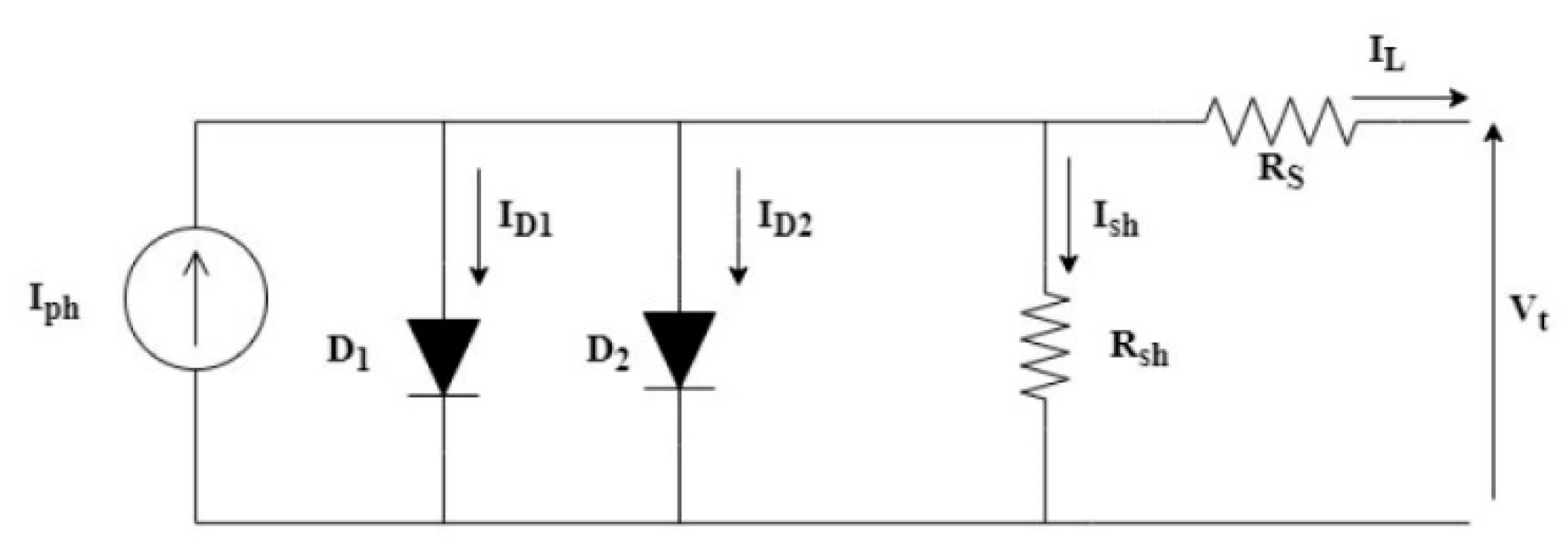
2.1.1. Single Diode Model (SDM) of a Solar Cell
The equivalent circuit of SDM is shown in Figure 1. The output current IL can be found out by using Equations (1)−(3).
where IL, Iph, Ish, I0, and ID are the output current from the solar cell equivalent circuit, the photo-current from the solar cell, current through the shunt resistance, reverse saturation current of the diode, and current through the diode, respectively. Rs and Rsh are the resistances connected in series and shunt branches, respectively. Vt is the voltage across the output terminal, n is the ideality factor, while k is the Boltzmann’s constant (1.380 × 10⁻²³ (J/K)). q (1.602 × 10⁻¹⁹ Coulumbs) is the magnitude of electronic charge. T is the absolute temperature of the solar cell in Kelvin.
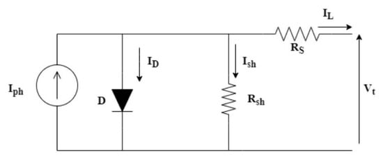
Figure 1.
Single Diode Model (SDM) of the solar PV cell.
The current IL can be found by substituting the values of the current through the diode (ID) from Equation (2) and the current through the shunt branch Ish from Equation (3) in Equation (1) as:
Equation (4) helps in finding out the unknown parameters, i.e., Rs, Rsh, I0, n1, and Iph of the solar cell with a single diode and obtain the characteristics of the cell closer to the actual one.
2.1.2. Double Diode Model (DDM) of a Solar Cell
The equivalent circuit of the double diode model can be represented as in Figure 2. It is different from SDM, with two diodes connected across the ideal current source. The output current of the solar cell, IL, can be found out using Kirchhoff’s Current Law and is expressed as:
where I01 and n1 are the reverse saturation current and ideality factor of diode D1 and I02, and n2 is the reverse saturation current and ideality factor of the diode D2.
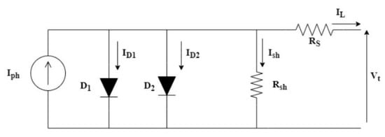
Figure 2.
Double Diode Model (DDM) of the solar PV cell.
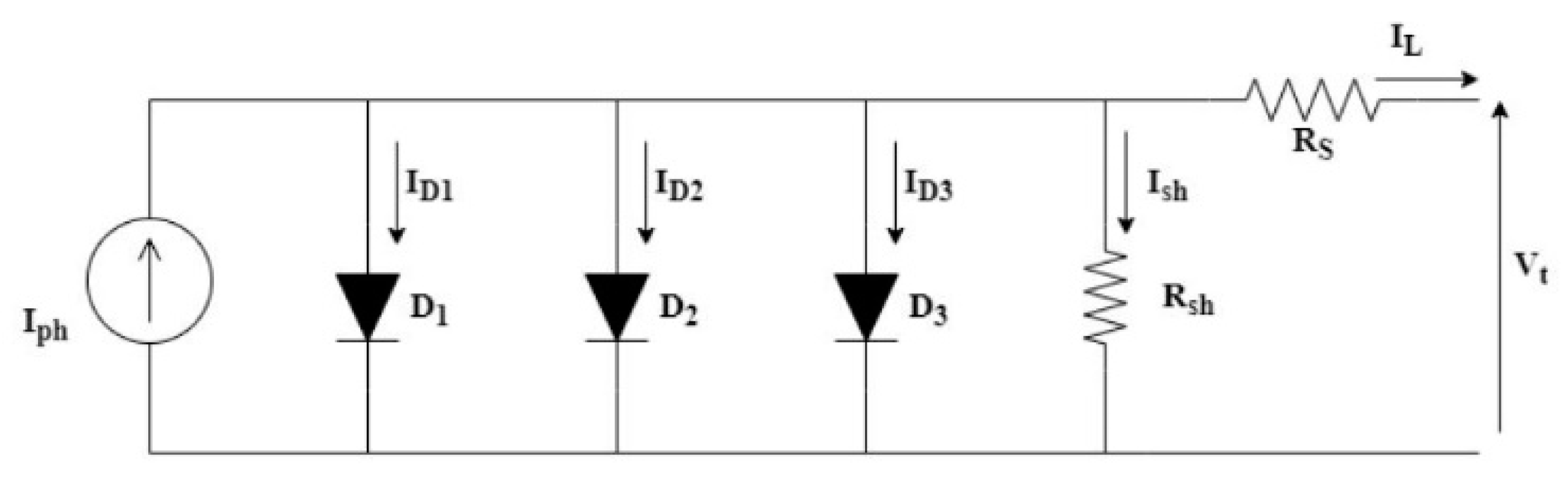
2.1.3. Three Diode Model (TDM) of a Solar Cell
The TDM can be represented as in Figure 3. This model has three diodes connected in parallel to the ideal current source along with resistances Rs and Rsh connected in series and parallel, respectively. The output current of the solar cell, IL, can be found out using KCL as:
where I01, I02, and I03 are the reverse saturation currents, while n1, n2, and n3 are the ideality factors of diodes D1, D2, and D3, respectively.
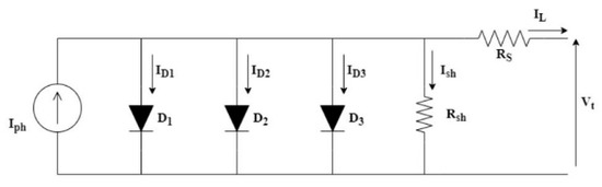
Figure 3.
Three Diode Model (TDM) of the PV cell.
The nine parameters of DDM, i.e., Rs, Rsh, I01, I02, I03, n1, n2, n3, and Iph, are aimed to be found out using Equation (8), with an aim to achieve the solar cell characteristics closer to the actual one.
2.2. Problem Formulation
The modeling of the solar PV systems is mainly aimed to obtain the unknown solar cell parameters of their respective equivalent circuits, i.e., SDM, DDM, or TDM. There must be only a minimum difference between the experimental data and data extracted from the algorithm.
The vital step in any optimization algorithm is determining the vector of solutions (Xi), the search range, and the objective function. The various vectors of the solution for SDM and DDM are shown in Table 3.
Table 3.
Vectors of solutions (Xi) for SDM and DDM.
This paper’s objective function is the Root Mean Square Error (RMSE) function and can be defined as the difference between the value of the estimated current from the algorithm and the value of the actual current extracted from the experiments.
For SDM the error function can be written as:
For DDM the error function can be written as:
For TDM the error function can be written as:
The Root Mean Square Error (RMSE) is the objective function and is mathematically defined as:
where N is the no. of readings of the measurement. The iteration stops once a decided number of steps is reached, or the error tolerance reaches a predefined value.
2.3. Chaotic Coyote Optimization Algorithm
In this work, a novel chaotic coyote optimization algorithm (COA) has been used for solving the objective function obtained in Equation (12). It is a metaheuristic algorithm and is inspired by incorporating chaos in the population generation in the coyote optimization presented in [46]. The coyote optimization is itself a social behavior and adaption of a species known as coyote/canis latrans presented in [46]. In the COA algorithm, the coyote population’s arrangement is so that there are Np groups of coyotes, and each group has Nc coyotes. The product of Np and Nc gives the total population of the species. Every individual coyote is a possible optimum solution for the optimization problem and its social conditions set (soc), which has all the decision variables included [46,47,48,49]. The Coyote Optimization Algorithm provides better parameter estimation of the solar PV module with lesser values of Root Mean Square Error than other mentioned techniques. However, when the algorithm gets aided with chaotic maps, there can be an appreciable improvement in the convergence speed of the results observed. The problem of getting trapped at the local optimum values, which is faced by other metaheuristic techniques, is overcome with the help of chaotic COA. The improvement of COA with the aid of ten different chaotic maps is shown in Section 3.2 of this paper for SDM, DDM, and TDM of various types of solar cell modules. The description of the coyote optimization and its subsequent modification to chaotic coyote has been discussed below:
The social condition of the cth coyote from the pth group at any instant is given in Equation (13) [47] as:
where J represents the dimension of the search space.
The adaptation of the coyote to its environment is the fitness function. The COA is started with the first step being the initialization of the global coyote population and are given by [47]:
where Lbj is the lower boundary, and Ubj is the upper boundary of the design variable j, and rj is any real random number between 0 and 1. The random number can better be replaced by chaotic numbers for better exploration of the search space. Thus, the following modification is done to Equation (14) [47].
where is the chaotic map function. For each coyote, the fitness function is written as [47]:
Sometimes at the beginning of COA, the coyotes might become solitary or join other groups, the probability of which is as follows [47]:
To avoid Pl exceeding the value of 1, Nc should be less than 14. In each pack, there is an alpha coyote that proves to have the maximum adaptation capability to the environment, is designated as ‘α’ and can be mathematically represented as [47]:
It is assumed that for the survival of the group, the coyote has to share its culture with other coyotes of the group, and this cultural tendency can be mathematically written as [47]:
where Opt is the ranked social status of the coyotes in group ‘p’ at time instant ‘t’ for j = 1, 2, 3, …D. The life events, such as the birth and the coyotes’ death, are taken into consideration by the COA. The birth of the coyotes is influenced by the social behavior of the two randomly selected parent coyotes of the same group and the environmental factors and can be mathematically represented as [47]:
where and are the coyotes selected randomly from the p-th group. j1 and j2 are the two random dimensions of the search space. Ps represents the probability of scattering, Pa represents the probability of association, Rj is a vector that is generated randomly, and randj is any number in the interval [0, 1] chosen randomly. The scattering probability and the association probability are represented as [47]:
and
It has been found that 10% of the young coyotes die at the time of birth. While the mortality rate of coyotes also increases with age. Algorithm 1 [48] shows the synchronism of the birth and the death of the coyotes (where ρ is the group that adjusts least to the environment than the young ones and ζ is the group of coyotes that adjusts less to the group size).
| Algorithm 1. Synchronism of the birth and the death of the coyotes. |
| Calculate ρ and ζ if ζ = 1 then retain the young coyote and eliminate the only coyote in ρ else if ζ > 1 then retain the young coyote and eliminate the oldest coyote in ρ else eliminate the young coyote end if |
The cultural interaction of coyotes within groups is shown with the help of d1 (it shows how the alpha influences a random coyote cr1) and d2 (showing how any random coyote cr2 is influenced by the cultural tendency of the group). cr1 and cr2 are selected using random probability distribution function, while d1 and d2 can be mathematically represented as:
and
The alpha coyote, as well as the other members of the group, affect the coyote’s social behavior, and the below equation gives the updated social condition:
where r1 and r2 are any real random numbers such that 0 ≤ r1, r2 ≤ 1. The new social behavior of the coyotes is estimated by:
Parameter Constraints
To extract the solar cell parameters, Equation (25) possesses an issue of causing the coyotes (parameters) to remain out of the already defined boundaries of the search and give impractical solutions. Therefore, to avoid this issue, an operator is introduced as in Equation (28). It helps in reinitializing the violating elements randomly within the search space.
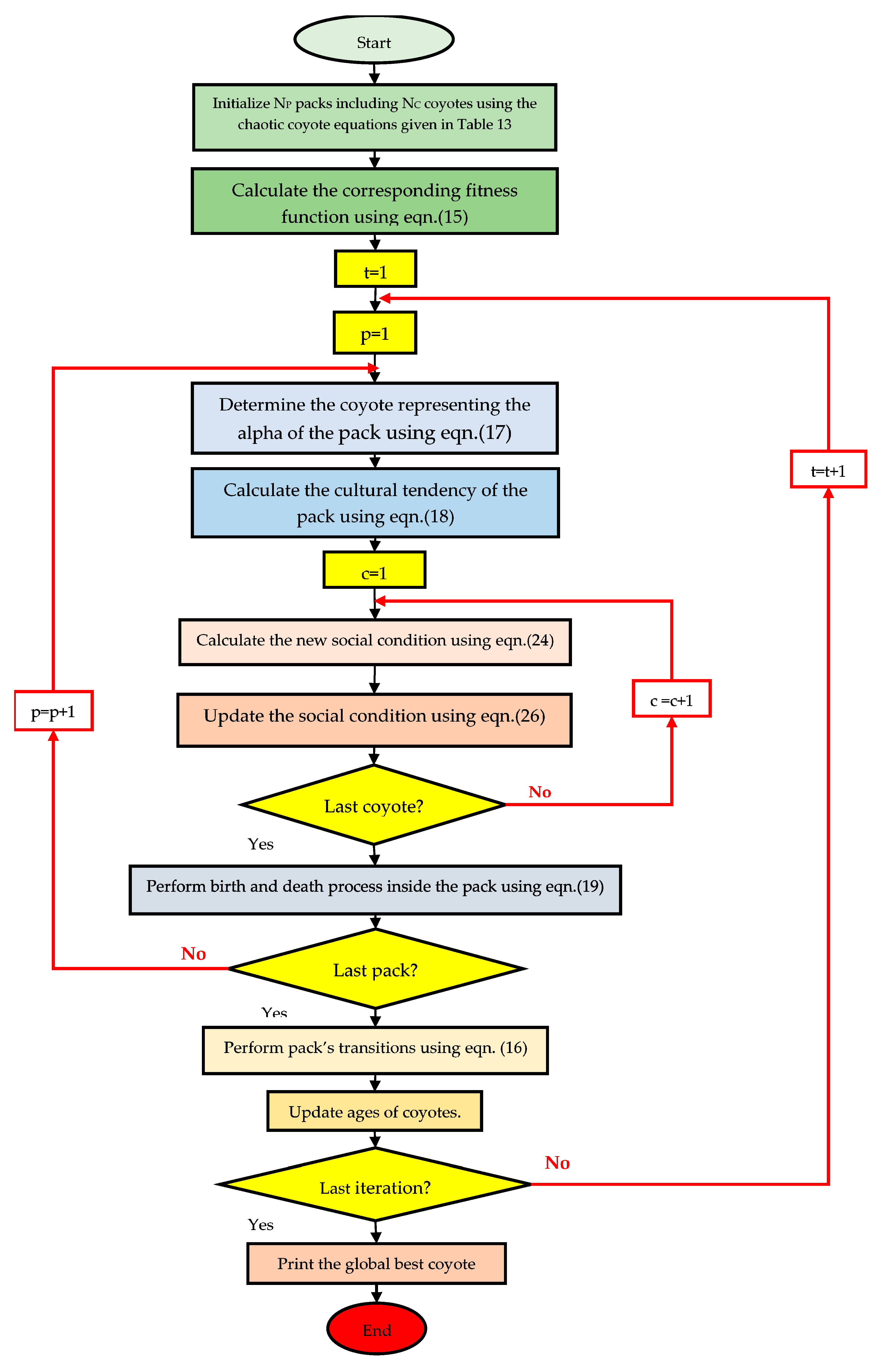
Algorithm 2 [48] shows the overall pseudo code to summarize the Chaotic COA. Chaotic COA is reiterated till a predefined criterion for stopping is met and the selection of that coyote is made, which adapts to the environment in a manner better than other coyotes. This coyote is selected as the Global Optimum Solution. The algorithm can also be observed from the flow chart shown in Figure 4.
| Algorithm 2. Chaotic COA. |
| Create Np packs with Nc coyotes in each pack using Equation (15) Assess the adaption of each coyote Equation (16) while stopping criteria satisfied do for each p pack do Find the pack’s alpha coyote Equation (18) for each cth coyote of pth pack do Generate new social conditions Equation (25) Check the boundary conditions Equation (28) Estimate the new social conditions Equation(26) Decide whether to move or not Equation (27) end for Simulate the birth and the death of the coyotes using Equation (20) and Algorithm 1 end for Impose the probabilities of coyotes leaving their packs using Equation (20) Update the coyotes’ ages endwhile Select the coyote with most potential to adapt to the environment. |

Figure 4.
Chaotic COA Flowchart.
3. Results and Discussions
In Section 3.1, the COA algorithm is applied to the parameters of different solar PV systems. The results are compared with other recent optimization techniques to prove the COA technique’s accuracy in the process of extraction of the parameters. Finally, in Section 3.2, chaotic coyote optimization has been taken for parameter extraction, and the results are obtained by comparing the various chaotic maps.
3.1. Results of COA with the Data from Experiments
The COA technique’s performance to extract solar PV parameters is done with the data observed from the experiments of [48] for a single diode model of PV cells. The COA algorithm is tested with three types of solar cells: mono-crystalline Leibold Solar Module (LSM 20) with 20 cells in series and at a temperature of 24 °C and irradiance of 360 W/m2, a Photowatt-PWP201 solar cell module with 36 polycrystalline silicon solar cells in series and a temperature of 45 °C and irradiance of 1000 W/m2, and a PVM752 GaAs thin-film solar cell at a temperature of 25 °C and irradiation of 1000 W/m2.
The extracted parameters are shown in Table 4, Table 5 and Table 6 for the single diode model (SDM) of mono-crystalline LSM20 module, Photowatt-PWP201 module, and PVM752, respectively. The parameter extraction performance by COA is compared with various recently proposed techniques, such as Differential Evolution (DE), Particle Swarm Optimization (PSO), and Particle Swarm Optimization and Gravitational Search Algorithm (PSOGSA).
Table 4.
Parameters extracted for a mono-crystalline LSM20 solar PV module by COA and its comparison with other techniques for SDM.
Table 5.
Parameters extracted for a Photowatt-PWP201 solar PV module by COA and its comparison with other techniques for SDM.
Table 6.
Parameters extracted for PVM752 GaAs thin-film solar PV cell by COA compared with other techniques for SDM.
As evident from Table 4, Table 5 and Table 6, COA provides lower RMSE values than other optimization techniques.
The comparison of various parameters along with their corresponding RMSE values and time of convergence for the double diode model and three diode model is shown in the Appendix A and Appendix B.
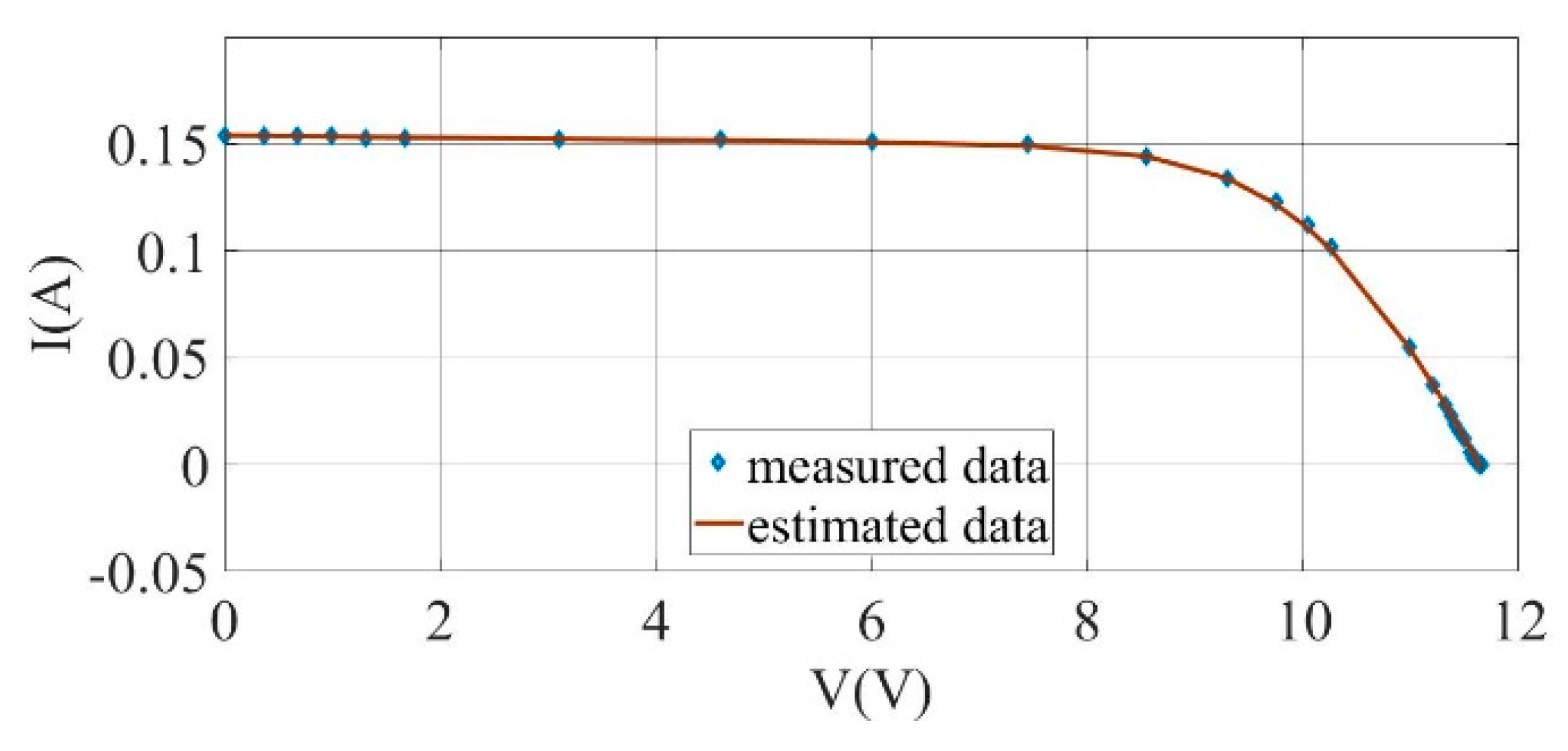
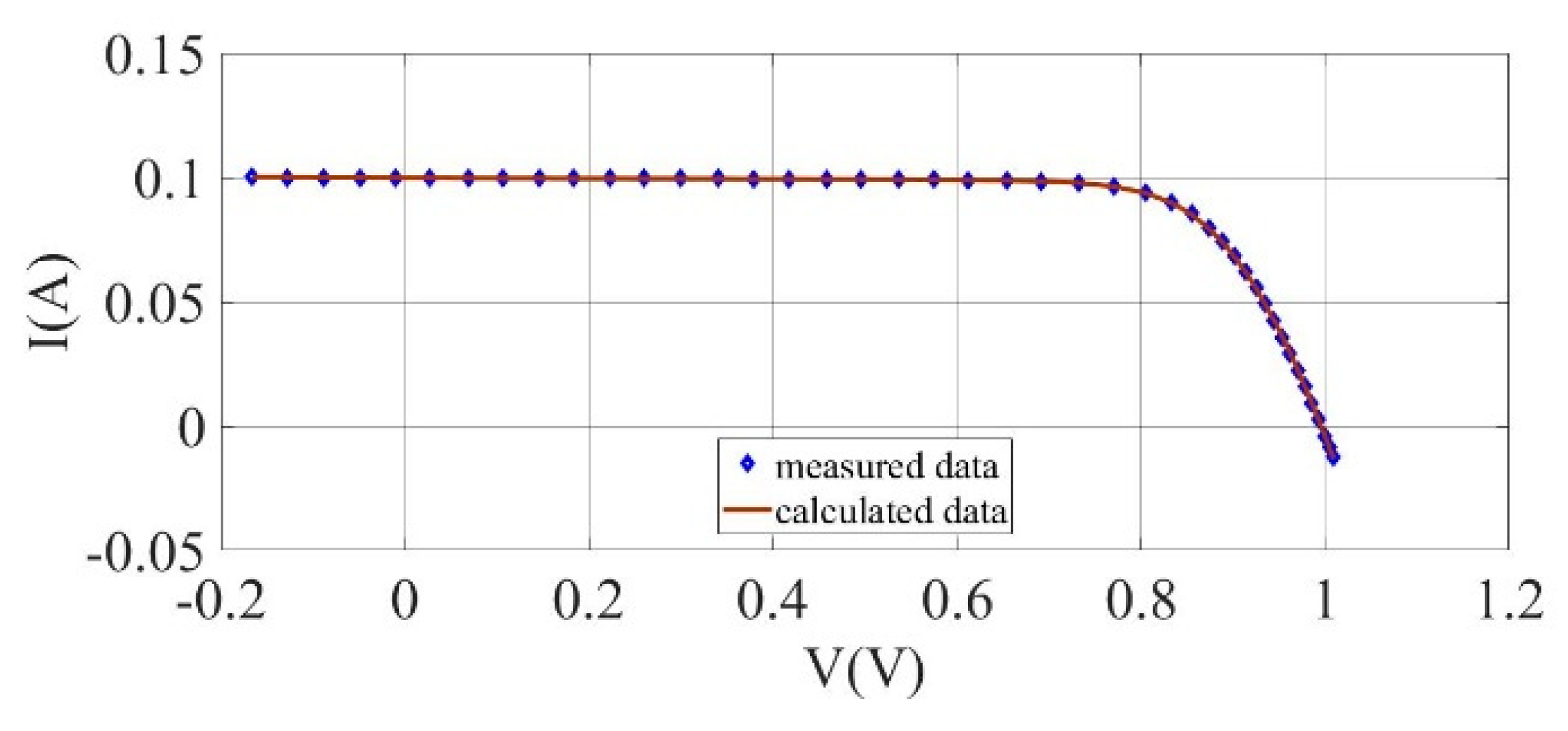
The I–V characteristics for the experimentally measured and calculated data are shown in Figure 5, Figure 6 and Figure 7 for the single diode model of mono-crystalline LSM20 solar cell module, Photowatt-PWP201 solar cell module, and GaAs thin-film solar cell.
Figure 5.
I–V curves for the experimentally measured data and the estimated results for a mono-crystalline LSM20 solar cell module (SDM).
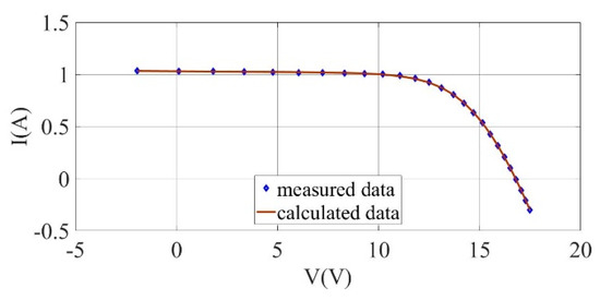
Figure 6.
I–V curves for the experimentally measured data and the estimated results for Photowatt-PWP201 solar cell module (SDM).
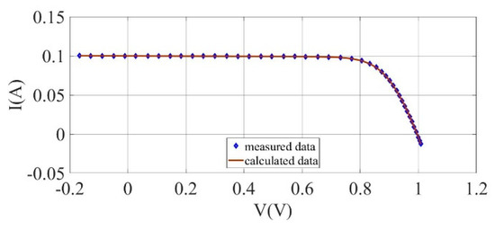
Figure 7.
I–V curves for the experimentally measured data and the estimated results for GaAs thin-film solar cell (SDM).
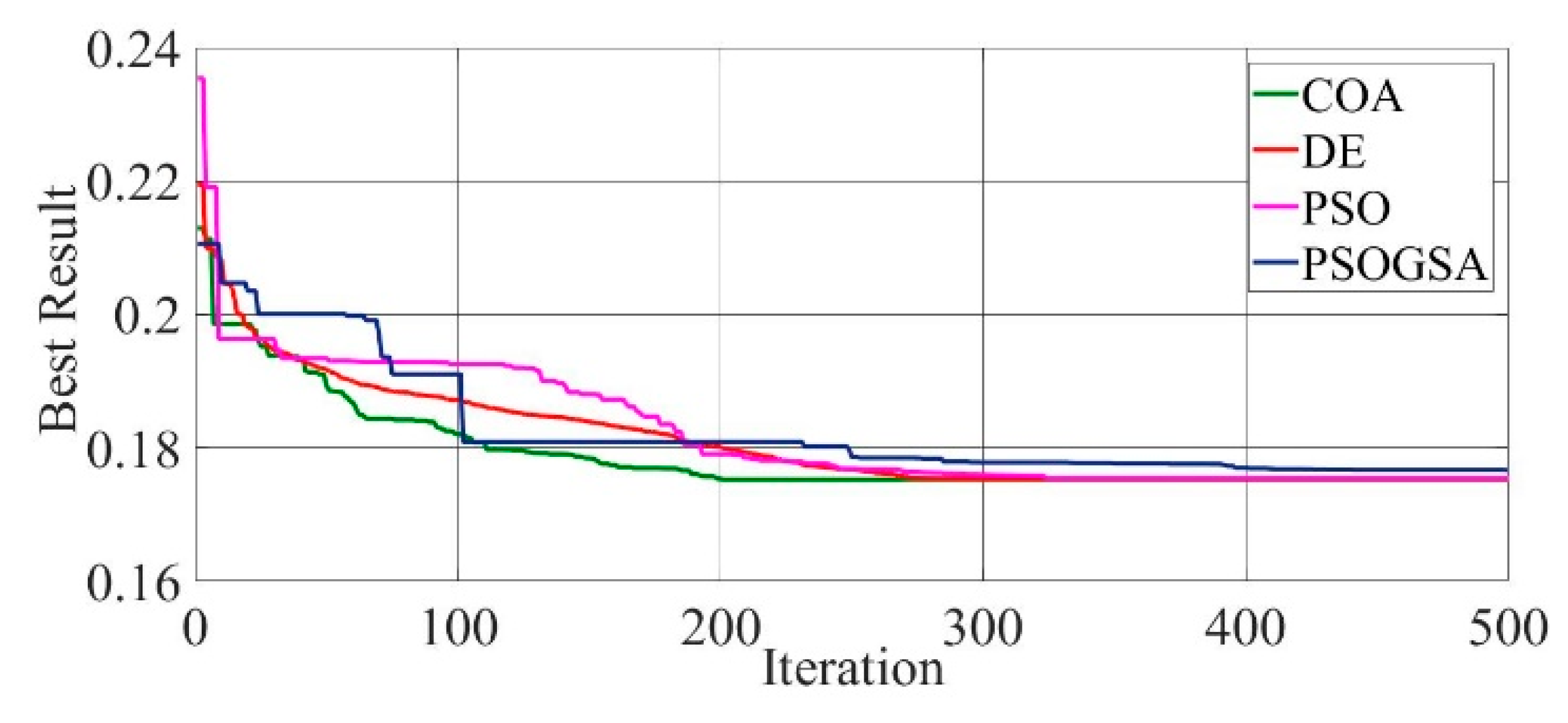
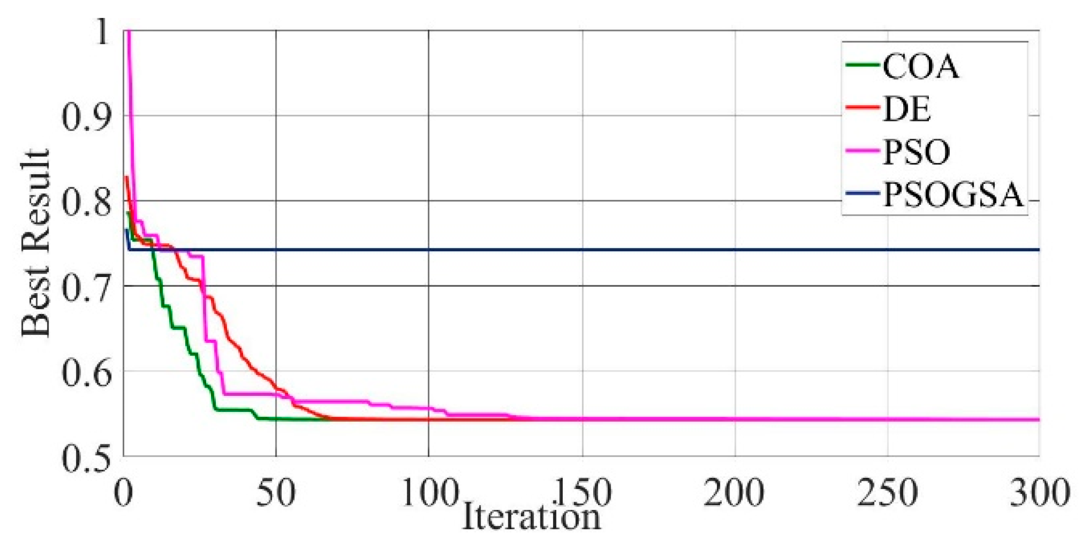
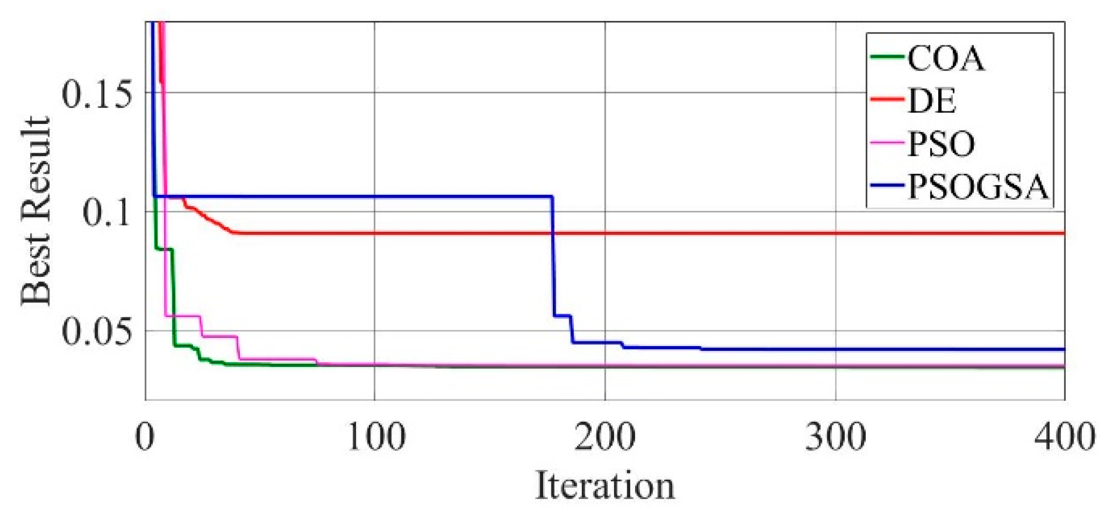
When the convergence curves of COA, DE, PSO, and PGSOSA are compared for the mono-crystalline LSM20 solar cell module (SDM), as shown in Figure 8, it can be observed that COA has the fastest convergence. The best values of optimal solution achieved are 0.1752, 0.175378, 0.17539, and 0.17667 in 215, 345, 465, and 500 iterations for COA, DE, PSO, and PSOGSA, respectively.
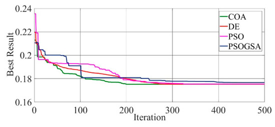
Figure 8.
Convergence curves of mono-crystalline LSM20 solar cell module (SDM) comparing the convergence characteristics of COA, DE, PSO, and PSOGSA.
When the convergence curves of COA, DE, PSO, and PGSOSA are compared for the Photowatt-PWP201 solar cell module (SDM), as shown in Figure 9, it can be observed that COA has the fastest convergence. The best values of optimal solution achieved are 0.5439, 0.5439, 0.5439, and 0.7424 in 70, 100, 280, and 8 iterations for COA, DE, PSO, and PSOGSA, respectively.
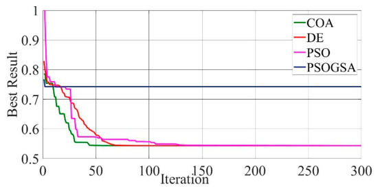
Figure 9.
Convergence curves of Photowatt-PWP201 solar cell module (SDM) comparing the convergence characteristics of COA, DE, PSO, and PSOGSA.
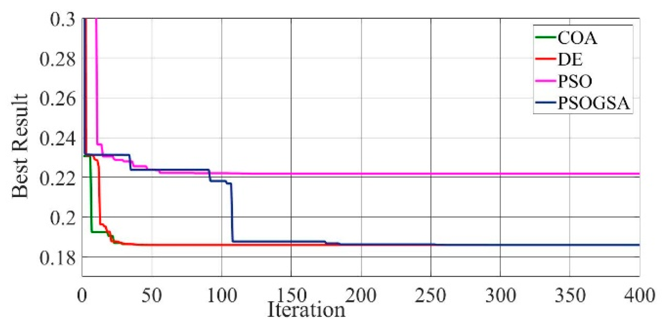
When the convergence curves of COA, DE, PSO, and PGSOSA are compared for GaAs thin-film solar cell-PVM752 (SDM), as shown in Figure 10, it can be observed that COA has the fastest convergence. The best values of optimal solution achieved are 0.185986, 0.85986, 0.22175, and 0.185986 in 45, 65, 130, and 385 iterations for COA, DE, PSO, and PSOGSA, respectively.
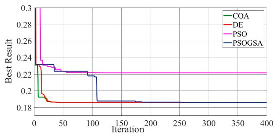
Figure 10.
Convergence curves of GaAs thin-film solar cell-PVM752 (SDM) comparing the convergence characteristics of COA, DE, PSO, and PSOGSA.
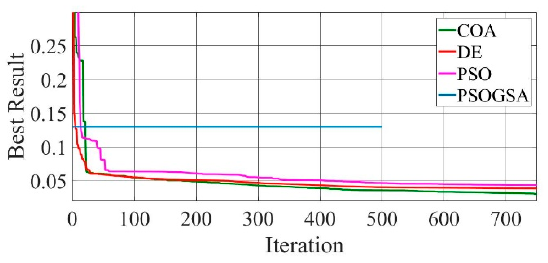
When the convergence curves of COA, DE, PSO, and PGSOSA are compared for a mono-crystalline LSM20 solar cell module (DDM), as shown in Figure 11, it can be observed that COA has the best convergence. The best values of optimal solution achieved are 0.02098, 0.030434, 0.05705, and 0.08679 in 400, 600, 130, and 10 iterations for COA, DE, PSO, and PSOGSA, respectively.
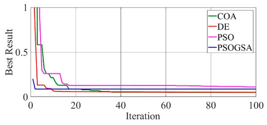
Figure 11.
Convergence curves of mono-crystalline LSM20 solar cell module (DDM) comparing the convergence characteristics of COA, DE, PSO, and PSOGSA.
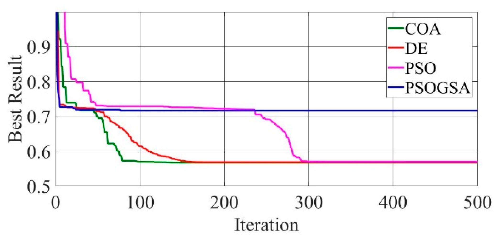
When the convergence curves of COA, DE, PSO, and PGSOSA are compared for Photowatt-PWP201 solar cell module (DDM), as shown in Figure 12, it can be observed that COA has the fastest convergence and lowest RMS error. The best values of optimal solution achieved are 0.5675, 0.56901, 0.57014, and 0.71649 in 150, 180, 300, and 150 iterations for COA, DE, PSO, and PSOGSA, respectively.

Figure 12.
Convergence curves of Photowatt-PWP201 solar cell module (DDM) comparing the convergence characteristics of COA, DE, PSO, and PSOGSA.
When the convergence curves of COA, DE, PSO, and PGSOSA are compared for GaAs thin-film solar cell-PVM752 (DDM), as shown in Figure 13, it can be observed that COA has the best convergence. The best values of optimal solution achieved are 0.034061, 0.090718, 0.034931, and 0.041737 in 120, 50, 300, and 350 iterations for COA, DE, PSO, and PSOGSA, respectively.
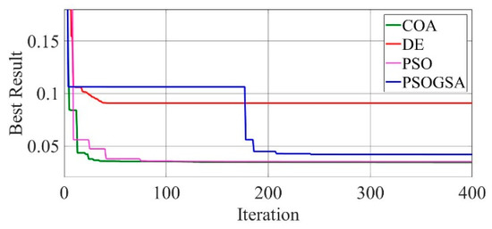
Figure 13.
Convergence curves of GaAs thin-film solar cell-PVM752 (DDM) comparing the convergence characteristics of COA, DE, PSO, and PSOGSA.
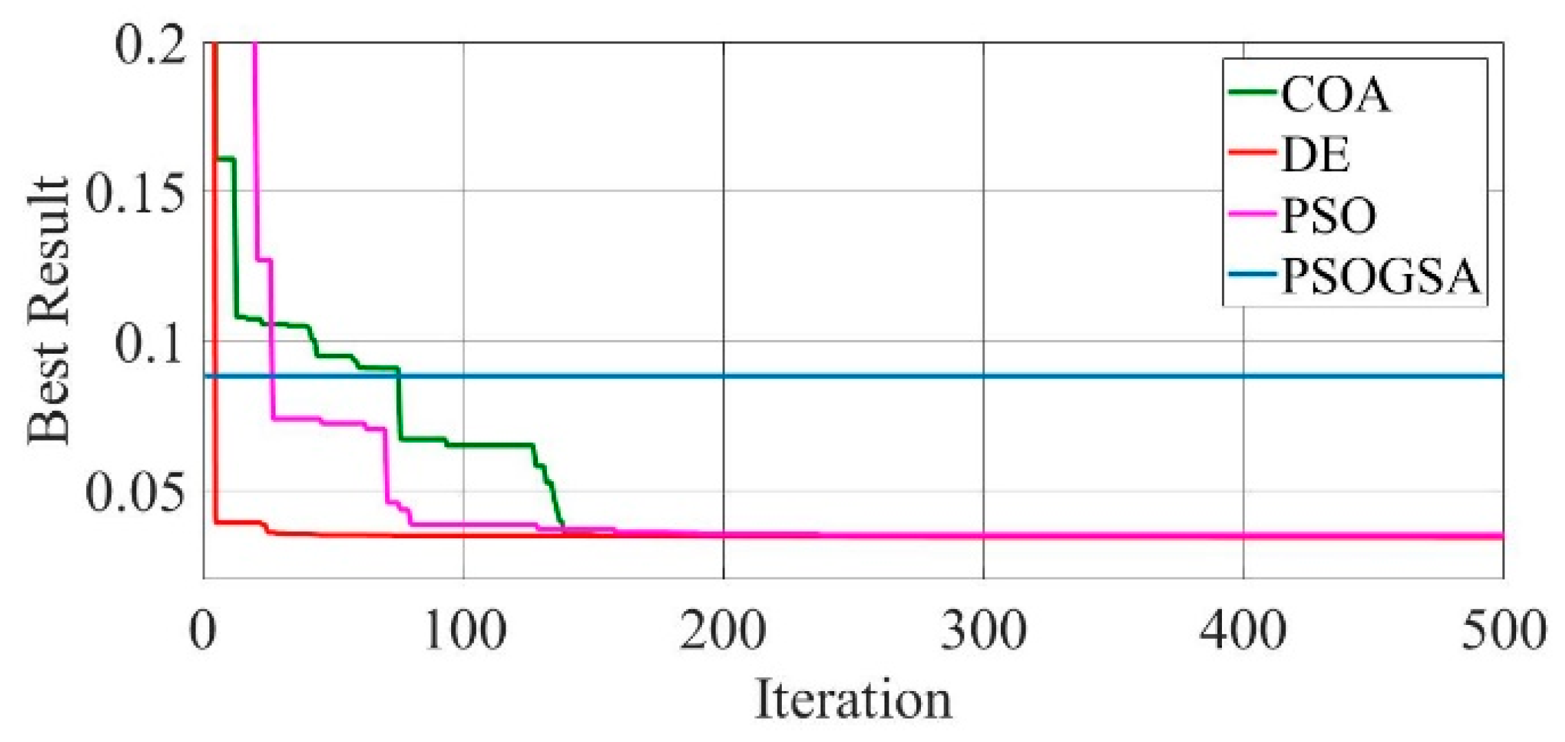
When the convergence curves of COA, DE, PSO, and PGSOSA are compared for a mono-crystalline LSM20 solar cell module (TDM), as shown in Figure 14, it can be observed that COA has the best convergence. The best values of optimal solution achieved are 0.026525, 0.034356, 0.04397, and 0.14497 in 400, 700, 730, and 10 iterations for COA, DE, PSO, and PSOGSA, respectively.
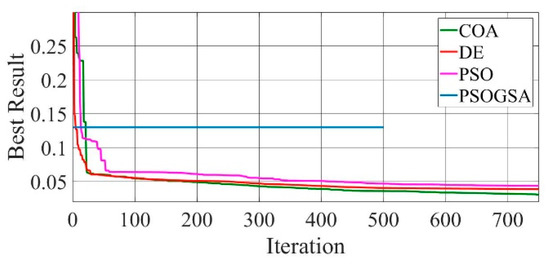
Figure 14.
Convergence curves of mono-crystalline LSM20 solar cell module (TDM) comparing the convergence characteristics of COA, DE, PSO, and PSOGSA.
When the convergence curves of COA, DE, PSO, and PGSOSA are compared for Photowatt-PWP201 solar cell module (TDM), as shown in Figure 15, it can be observed that COA has the fastest convergence and lowest RMS error. The best values of optimal solution achieved are 0.569033, 0.567506, 0.569564, and 0.93278 in 125, 200, 250, and 10 iterations for COA, DE, PSO, and PSOGSA, respectively.
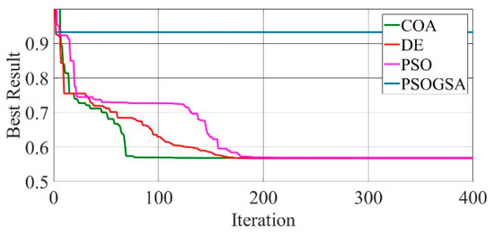
Figure 15.
Convergence curves of Photowatt-PWP201 solar cell module (TDM) comparing the convergence characteristics of COA, DE, PSO and PSOGSA.
When the convergence curves of COA, DE, PSO, and PGSOSA are compared for GaAs thin-film solar cell-PVM752 (DDM), as shown in Figure 16, it can be observed that COA has the best convergence. The best values of optimal solution achieved are 0.03483, 0.034061, 0.3503, and 0.088164 in 150, 450, 250, and 10 iterations for COA, DE, PSO, and PSOGSA, respectively.
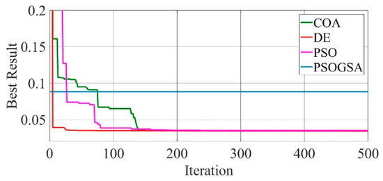
Figure 16.
Convergence curves of GaAs thin-film solar cell-PVM752 (TDM) comparing the convergence characteristics of COA, DE, PSO, and PSOGSA.
3.2. Parameter Extraction Using Coyote Optimization Algorithm with Chaotic Maps
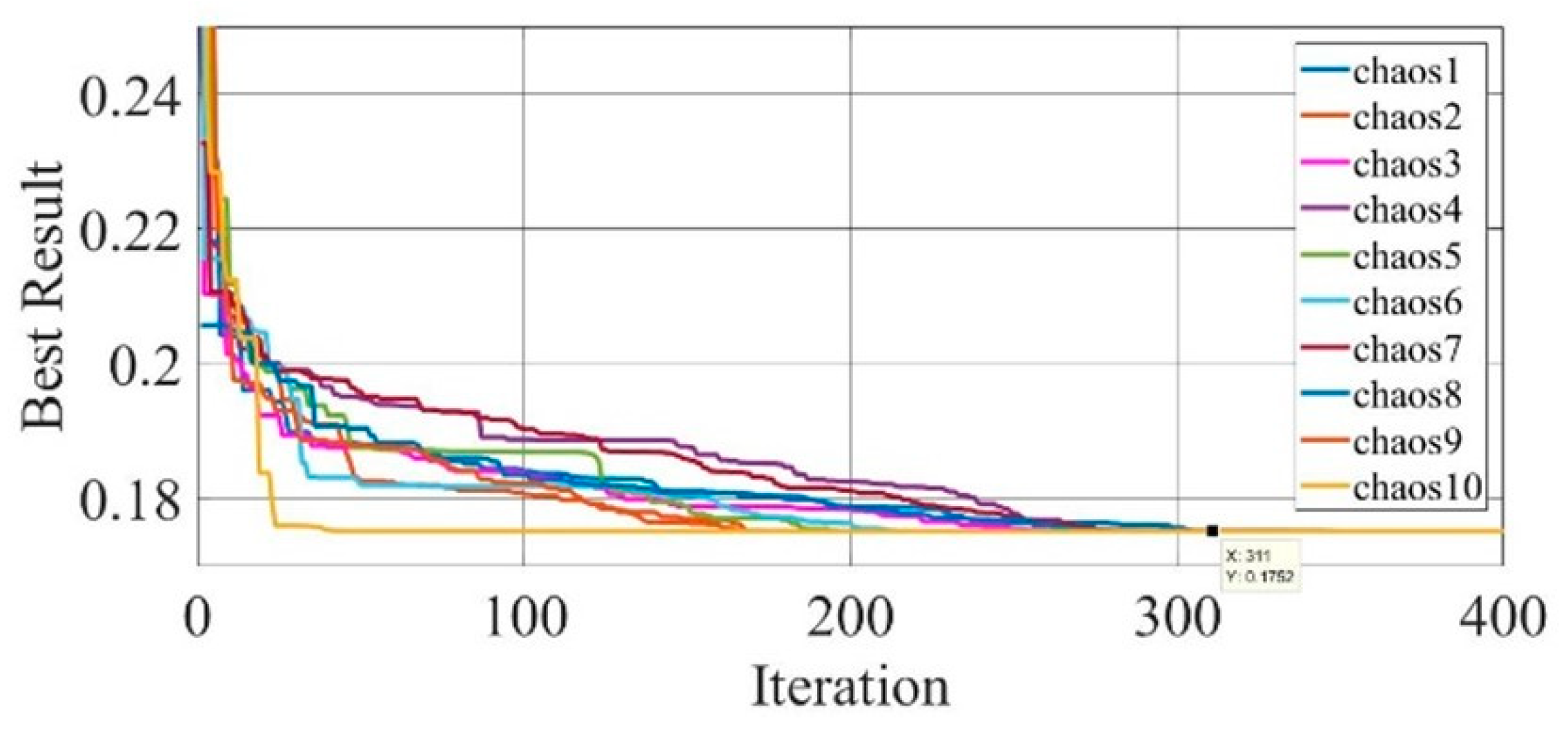
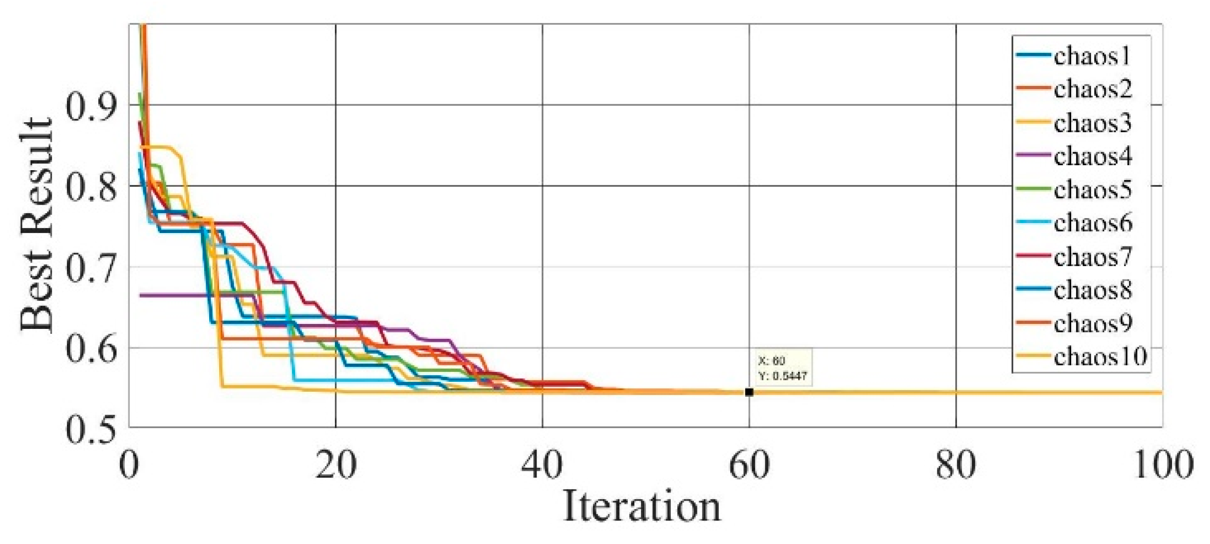
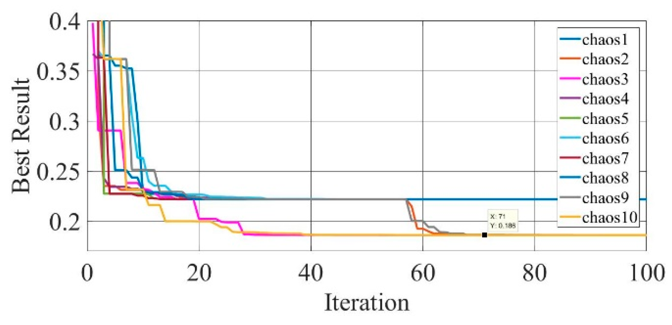
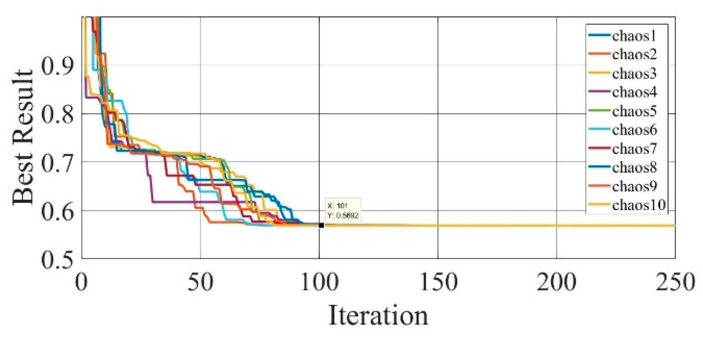
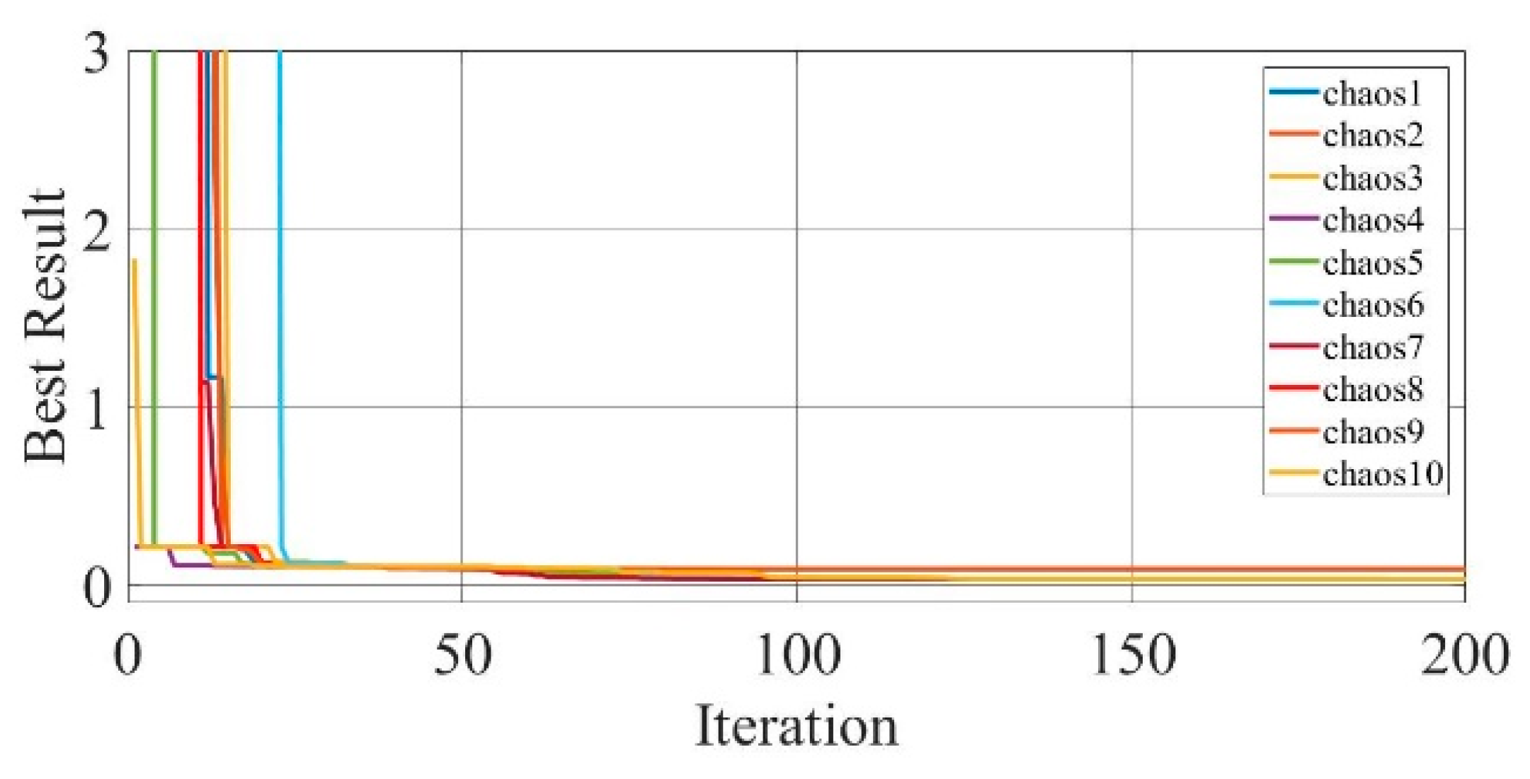
With the help of chaotic methods, the performance of the COA technique can be improved considerably as the convergence speed can be increased, and the problem of local optimum can be avoided. In this paper, ten chaotic maps are used in order to improve the performance of the COA [52]. Table 7 shows the enumeration of the chaotic functions used in this paper [52]. It is also observed that COA with chaos is faster with a very high convergence speed, which is evident from the convergence curves for the ten chaotic functions in Figure 17, Figure 18 and Figure 19, for a mono-crystalline LSM20 solar cell module, Photowatt-PWP201 solar cell module, and GaAs thin-film solar cell PVM752 respectively, where the chaos maps are named as chaos1, chaos2, …, chaos10 in accordance with Table 7.
Table 7.
Chaos Table.
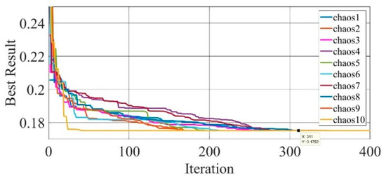
Figure 17.
Convergence curves of chaotic COA optimization technique during parameter extraction for a mono-crystalline solar cell LSM20 module (SDM).
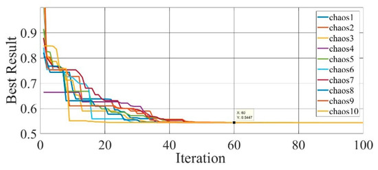
Figure 18.
Convergence curves of chaotic COA optimization technique during parameter extraction for Photowatt-PWP201 solar cell module (SDM).
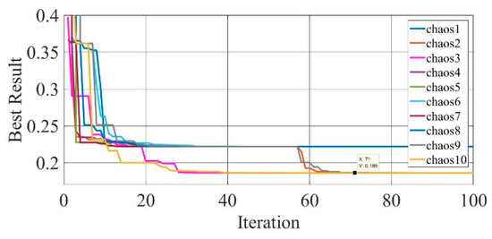
Figure 19.
Convergence curves of chaotic COA optimization technique during parameter extraction for GaAs thin-film solar cell PVM752 (SDM).
The applications of various metaheuristic methods in Solar PV parameter extraction and other industrial application has been discussed in [62,63,64,65,66,67,68].
3.2.1. Chaotic COA for Single Diode Model
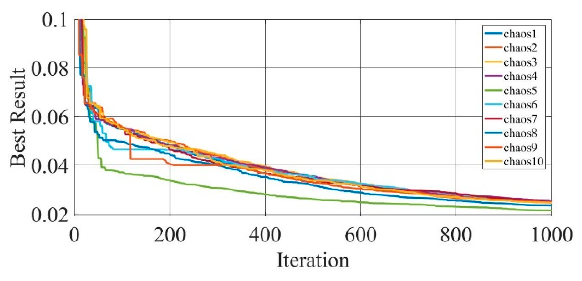
Figure 17 shows that the COA with chaos achieves the optimal value of 0.175235 for the LSM20 solar module in 310 iterations, which is much less than the COA without the chaos. Furthermore, the time taken by each chaotic map to converge and reach the optimal value of 0.175235 is shown in Table 8.
Table 8.
Time taken by COA with the ten chaotic functions for LSM20 solar module.
Figure 18 shows that the COA with chaos achieves the optimal value of 0.5447 for the Photowatt-PWP 201 solar cell module in 60 iterations, which is much less than the COA without the chaos. Furthermore, each chaotic map’s time is shown in Table 9.
Table 9.
Time taken by COA with the ten chaotic functions for Photowatt-PWP201 solar cell module (SDM).
Figure 19 shows that the COA with chaos achieves the optimal value of 0.1866 for GaAs thin-film solar cell PVM752 in 70 iterations, which is much less than the COA without the chaos. Furthermore, the time taken by each chaotic map is shown in Table 10.
Table 10.
Time taken by COA with the ten chaotic functions for GaAs thin-film solar cell PVM752 (SDM).
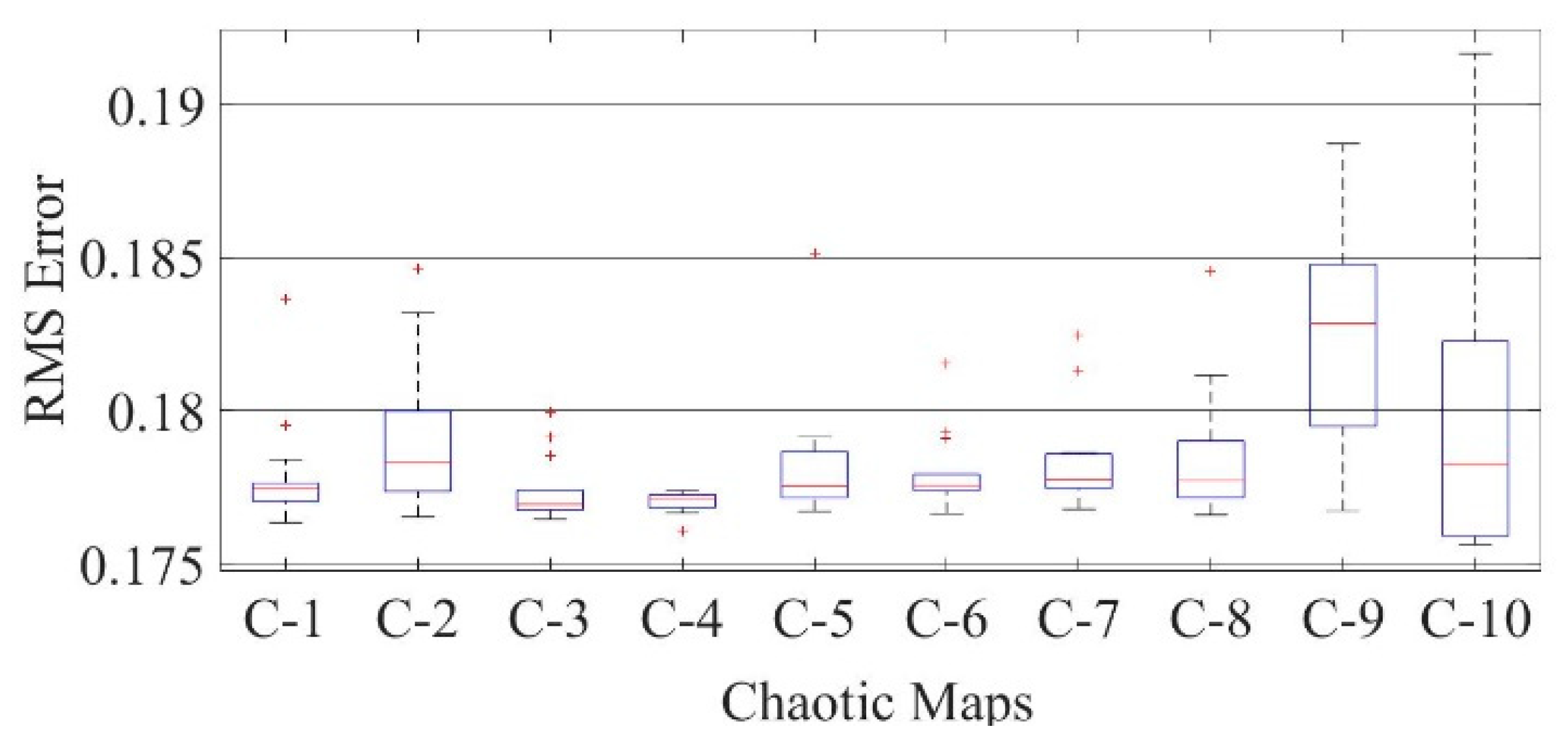
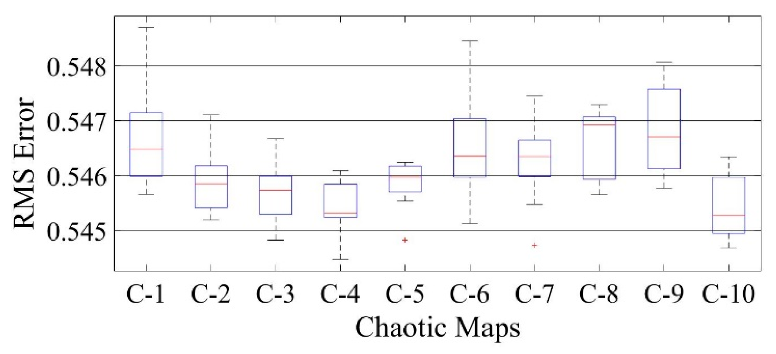
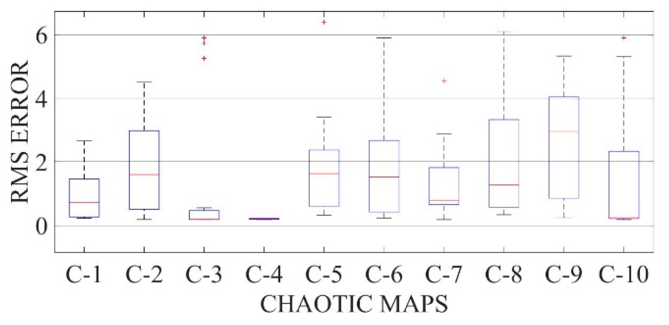
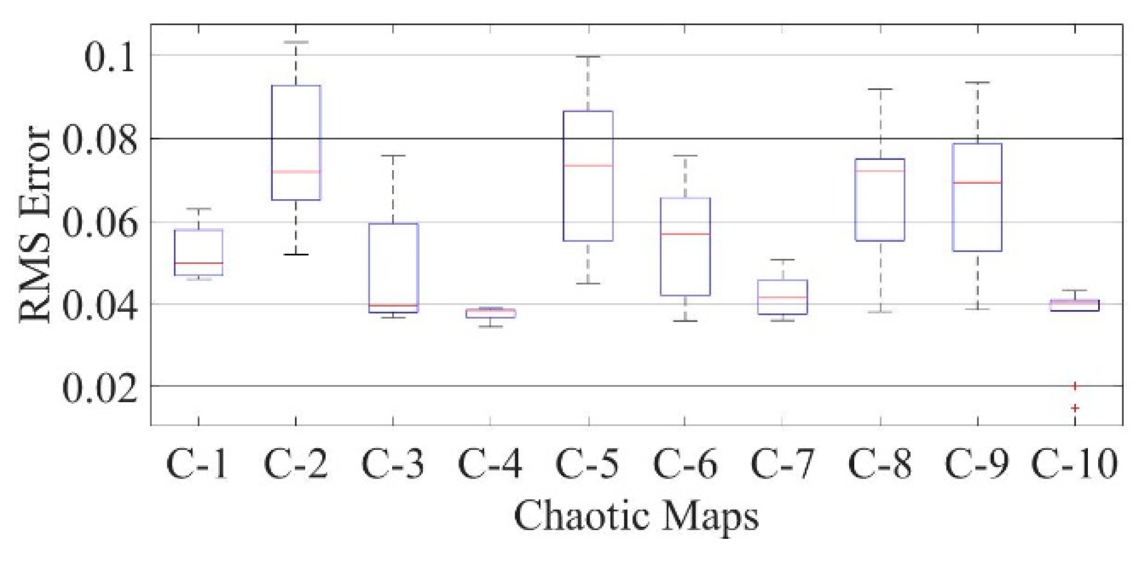
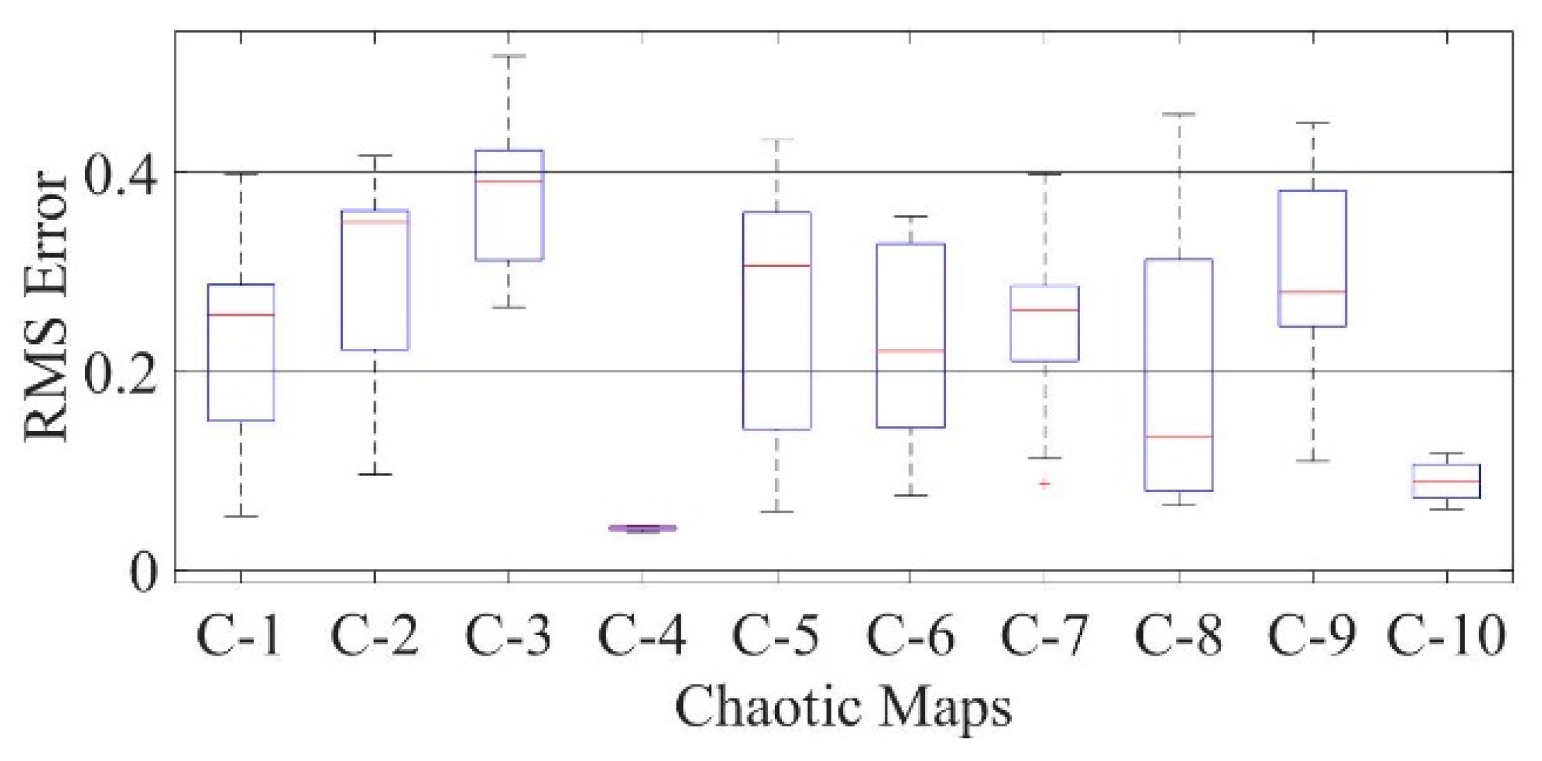
Chaotic functions are used with the Coyote Optimization Algorithm in order to attain improved results with a higher convergence speed. The effect of the ten chaotic functions on the RMSE values using COA are shown with the help of boxplots for single diode models of mono-crystalline LSM20 solar module in Figure 20, Photowatt-PWP201 solar cell module in Figure 21, and for GaAs thin-film solar cell module in Figure 22, which shows that the results are better than using COA alone. The various chaotic functions mentioned in Table 7 are represented as C-N’ in the boxplot, such that 1 ≤ N’ ≤ 10, (where N’ is the serial number of the chaotic maps mentioned in Table 7).
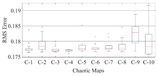
Figure 20.
Boxplot comparing RMSE values using COA with the help of chaotic maps for a mono-crystalline LSM20 solar cell module (SDM).
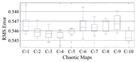
Figure 21.
Boxplot comparing RMSE values using COA with the help of chaotic maps for a polycrystalline PWP-201 solar cell module (SDM).

Figure 22.
Boxplot comparing RMSE values using COA with the help of chaotic maps for a thin-film solar cell PVM752 (SDM).
For a mono-crystalline LSM20 solar cell module (SDM), the median value of RMSE were found as 0.17635, 0.17652, 0.17645, 0.17608, 0.17671, 0.17663, 0.17678, 0.17659, 0.17672, and 0.17563, respectively, for various chaotic functions as in the order given in Table 7.
For a polycrystalline Photowatt-PWP201 solar cell module (SDM), the median RMSE values were 0.54566, 0.5452, 0.54483, 0.54447, 0.54483, 0.54513, 0.54473, 0.54566, 0.54577, and 0.54469, respectively, for various chaotic functions as in the order given in Table 7.
In the case of thin-film solar cell PVM752 (SDM), the median RMSE values were obtained as 0.22546, 0.18823, 0.18739, 0.18665, 0.32785, 0.23471, 0.18718, 0.33825, 0.24396, and 0.18645, respectively, for various chaotic functions as in the order of Table 7.
3.2.2. Chaotic COA for Double Diode Model
Figure 23 shows that the COA with chaos achieves the optimal value of 0.020908 for the LSM20 solar module (DDM) in 800 iterations, which is much less than the COA without the chaos. Furthermore, each chaotic map’s time to converge and reach the optimal value of 0.020908 is shown in Table 11.

Figure 23.
Convergence curves of chaotic COA optimization technique during parameter extraction for a mono-crystalline solar cell LSM20 module (DDM).
Table 11.
Time taken by COA with the ten chaotic functions for LSM20 solar module (DDM).
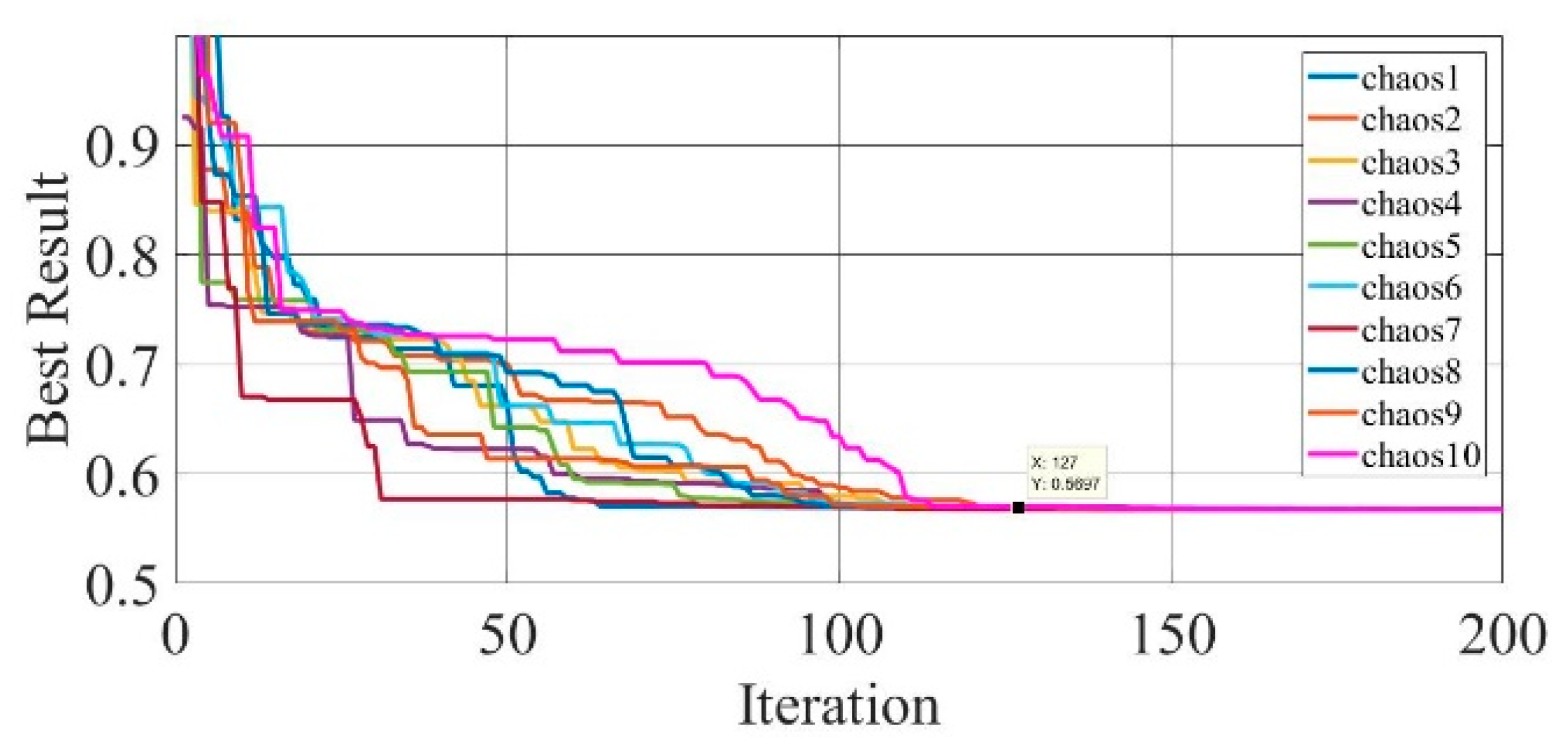
Figure 24 shows that the COA with chaos achieves the optimal value of 0.5697 for the Photowatt-PWP 201 solar cell module (DDM) in 127 iterations, which is much less than the COA without the chaos. Furthermore, each chaotic map’s time is shown in Table 12.

Figure 24.
Convergence curves of chaotic COA optimization technique during parameter extraction for Photowatt-PWP201 solar cell module (DDM).
Table 12.
Time taken by COA with the ten chaotic functions for Photowatt-PWP201 solar cell module (DDM).
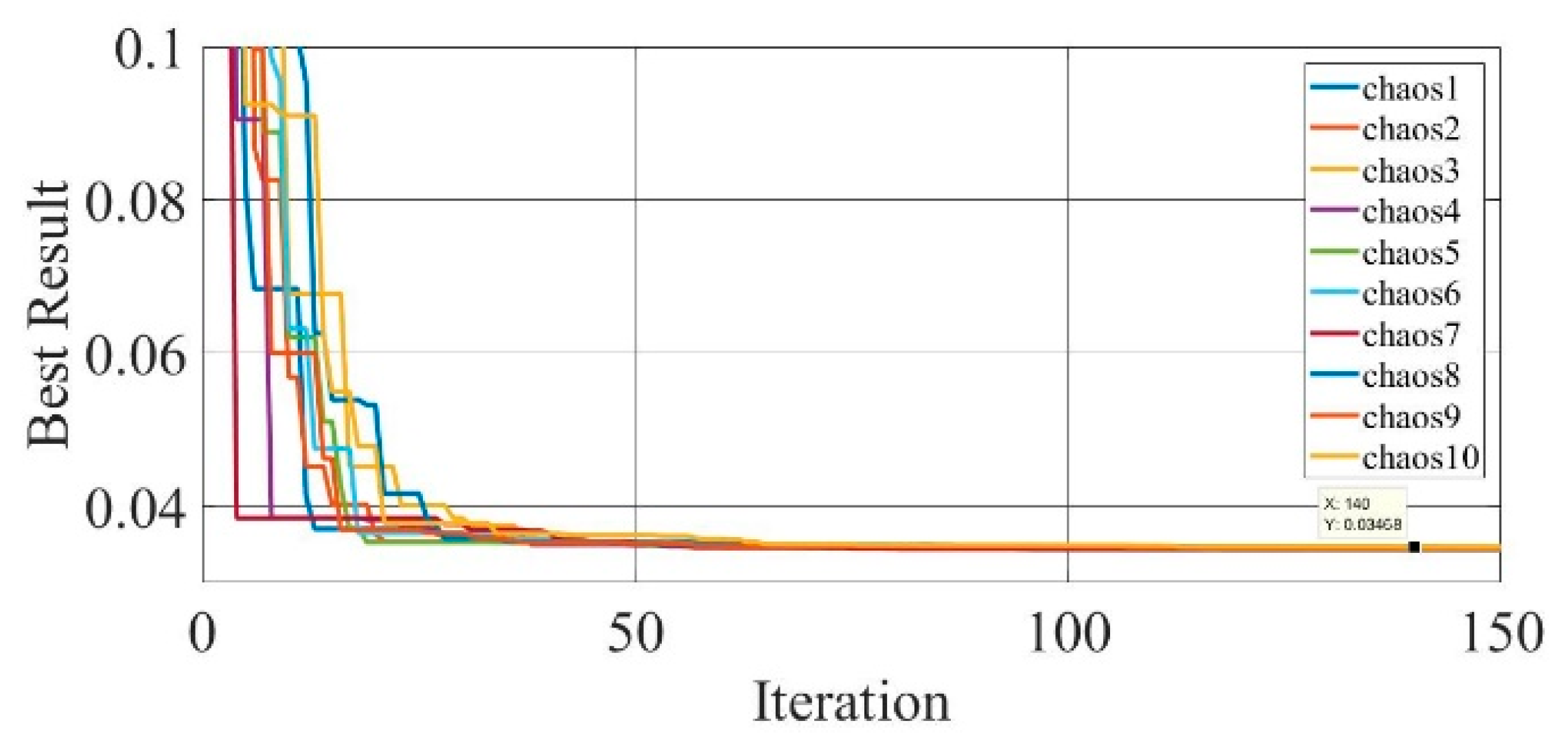
Figure 25 shows that the COA with chaos achieves the optimal value of 0.03468 for GaAs thin-film solar cell PVM752 in 140 iterations, which is much less than the COA without the chaos. Furthermore, each chaotic map’s time is shown in Table 13.
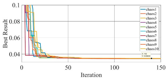
Figure 25.
Convergence curves of chaotic COA optimization technique during parameter extraction for GaAs thin-film solar cell PVM752 (DDM).
Table 13.
Time taken by COA with the ten chaotic functions for GaAs thin-film solar cell PVM752 (DDM).
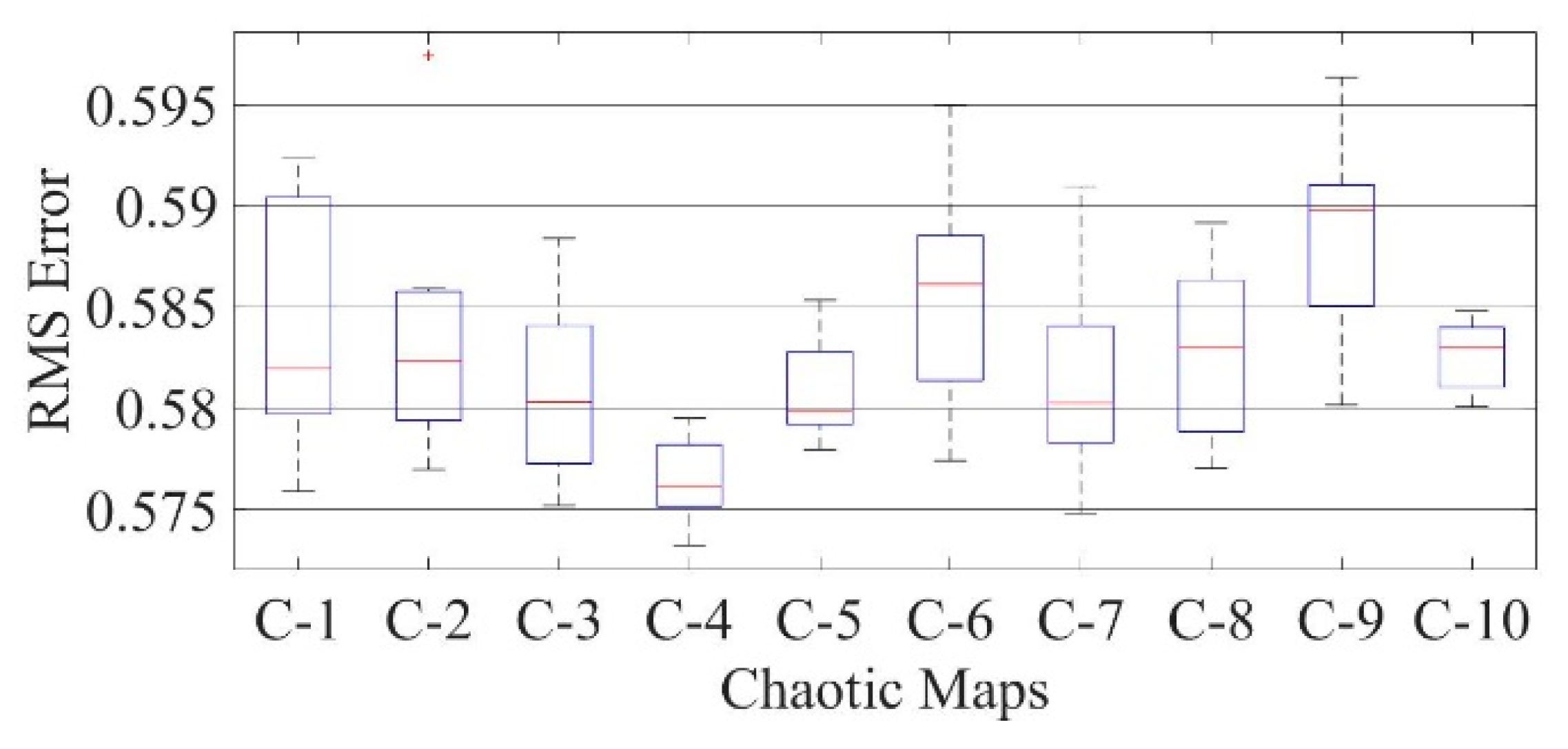
The effect of the ten chaotic functions on the RMSE values using COA is shown with the help of boxplots for double diode models of mono-crystalline LSM20 solar module in Figure 26, Photowatt-PWP201 solar cell module in Figure 27, and for GaAs thin-film solar cell module in Figure 28, which shows that the results are better in most of the chaotic maps when compared to using COA alone.
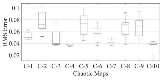
Figure 26.
Boxplot comparing RMSE values using COA with the help of chaotic maps for a mono-crystalline LSM20 solar cell module (DDM).

Figure 27.
Boxplot comparing RMSE values using COA with the help of chaotic maps for a polycrystalline PWP-201 solar cell module (DDM).
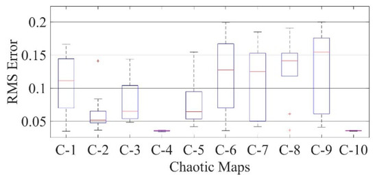
Figure 28.
Boxplot comparing RMSE values using COA with the help of chaotic maps for a thin-film solar cell PVM752 (DDM).
For a mono-crystalline LSM20 solar cell module (DDM), the median value of RMSE were found as 0.049869, 0.071838, 0.039428, 0.038175, 0.073488, 0.056864, 0.041471, 0.071894, 0.069284, and 0.04194, respectively, for various chaotic functions as in the order given in Table 7.
For a polycrystalline Photowatt-PWP201 solar cell module (DDM), the median RMSE values were 0.58195, 0.58233, 0.58031, 0.57613, 0.57982, 0.58613, 0.58026, 0.58301, 0.5898, and 0.58297, respectively, for various chaotic functions as in the order given in Table 7.
In the case of thin-film solar cell PVM752 (DDM), the median RMSE values were obtained as 0.11121, 0.051876, 0.06504, 0.035617, 0.064541, 0.1275, 0.1251, 0.14145, 0.15479, and 0.035838, respectively, for various chaotic functions as in the order of Table 7.
3.2.3. Chaotic COA for the Three Diode Model
Figure 29 shows that the COA with chaos achieves the optimal value of 0.026525 for the LSM20 solar module (TDM) in 750 iterations, which is much less than the COA without the chaos. Furthermore, each chaotic map’s time to converge and reach the optimal value is shown in Table 14.
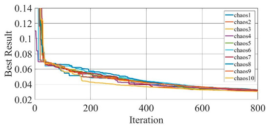
Figure 29.
Convergence curves of chaotic COA optimization technique during parameter extraction for a mono-crystalline solar cell LSM20 module (TDM).
Table 14.
Time taken by COA with the ten chaotic functions for LSM20 solar module (TDM).
Figure 30 shows that the COA with chaos achieves the optimal value of 0.5692 for the Photowatt-PWP 201 solar cell module (DDM) in 100 iterations, which is much less than the COA without the chaos. Furthermore, each chaotic map’s time is shown in Table 15.
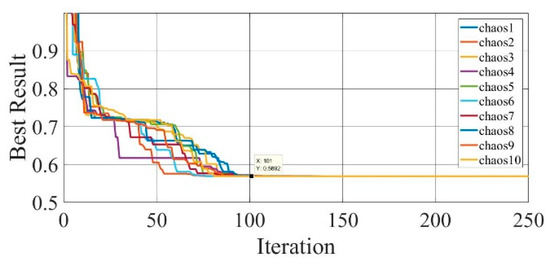
Figure 30.
Convergence curves of chaotic COA optimization technique during parameter extraction for Photowatt-PWP201 solar cell module (TDM).
Table 15.
Time taken by COA with the ten chaotic functions for Photowatt-PWP201 solar cell module (TDM).
Figure 31 shows that the COA with chaos achieves the optimal value of 0.034863 for GaAs thin-film solar cell PVM752 in 150 iterations, which is much less than the COA without the chaos. Furthermore, each chaotic map’s time is shown in Table 16.
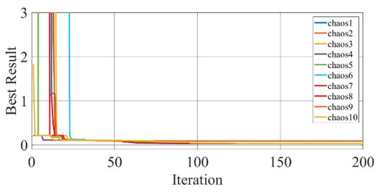
Figure 31.
Convergence curves of chaotic COA optimization technique during parameter extraction for GaAs thin-film solar cell PVM752 (TDM).
Table 16.
Time taken by COA with the ten chaotic functions for GaAs thin-film solar cell PVM752 (TDM).
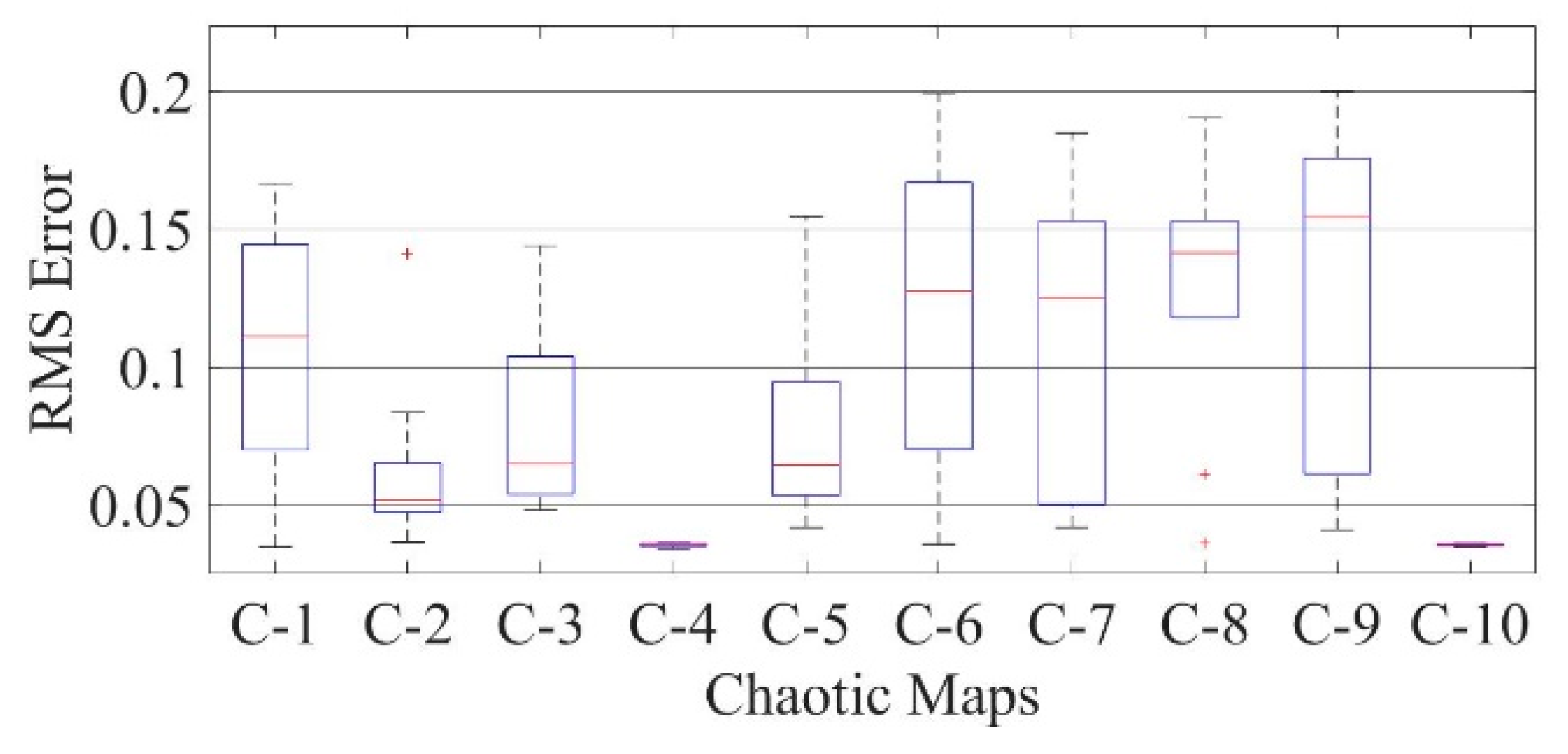
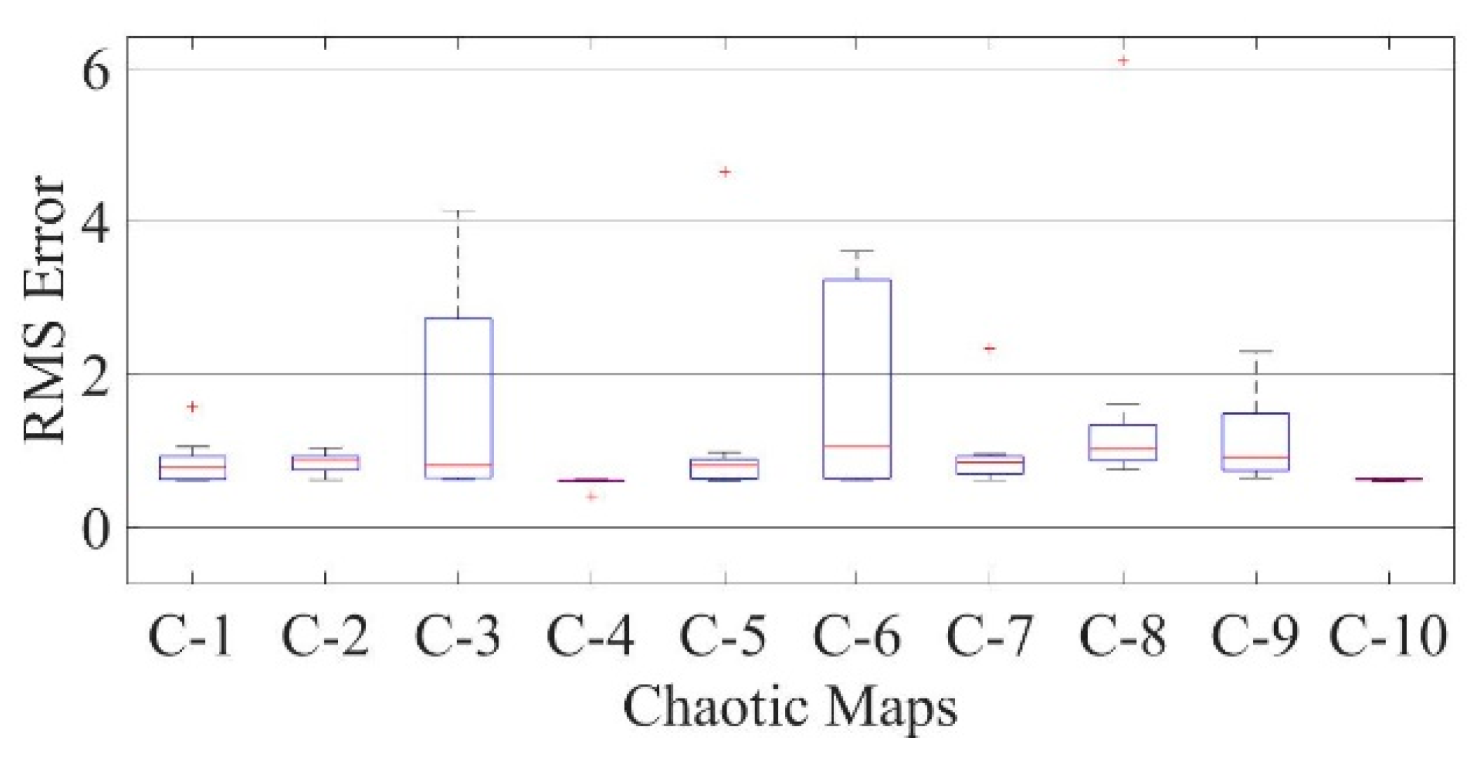
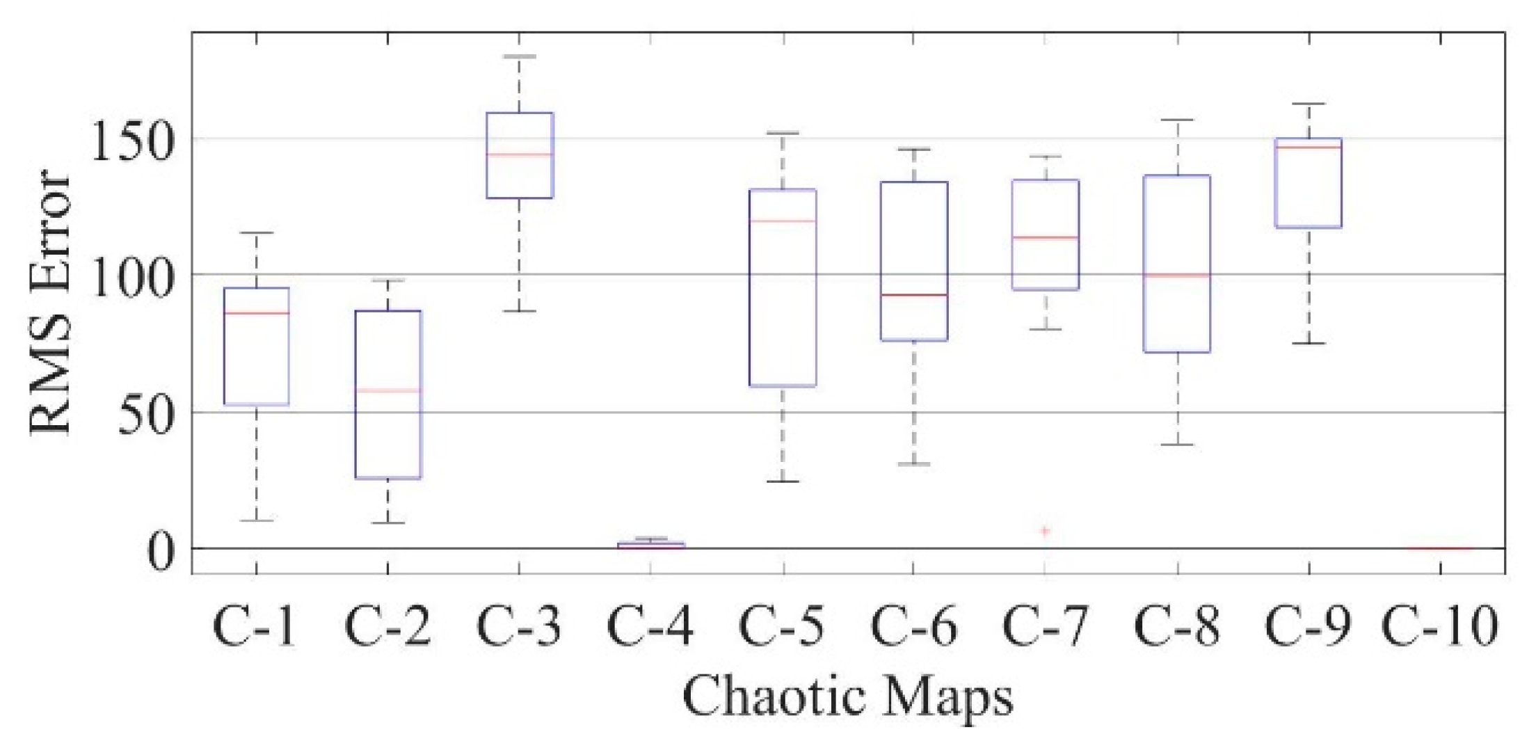
The effect of the ten chaotic functions on the RMSE values using COA is shown with the help of boxplots for double diode models of mono-crystalline LSM20 solar module in Figure 32, Photowatt-PWP201 solar cell module in Figure 33, and for GaAs thin-film solar cell module in Figure 34, which shows that the results are better than using COA alone.
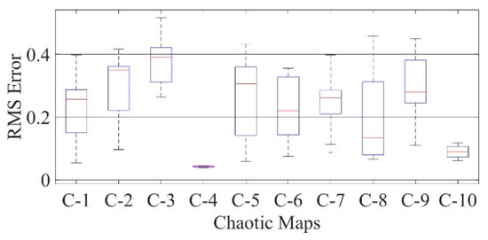
Figure 32.
Boxplot comparing RMSE values using COA with the help of chaotic maps for a mono-crystalline LSM20 solar cell module (TDM).
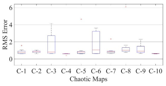
Figure 33.
Boxplot comparing RMSE values using COA with the help of chaotic maps for a polycrystalline PWP-201 solar cell module (TDM).
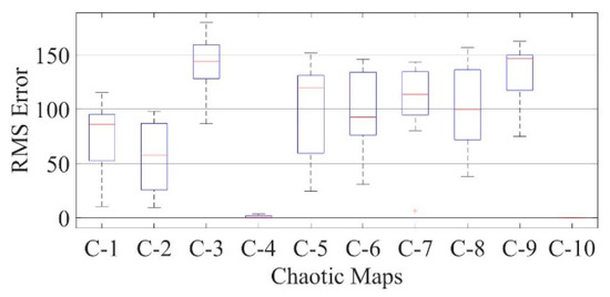
Figure 34.
Boxplot comparing RMSE values using COA with the help of chaotic maps for a thin-film solar cell PVM752 (TDM).
For a mono-crystalline LSM20 solar cell module (TDM), the median values of RMSE were found as 0.25648, 0.35002, 0.39102, 0.042622, 0.30653, 0.22045, 0.26169, 0.13361, 0.27937, and 0.0895, respectively, for various chaotic functions as in the order given in Table 7.
For a polycrystalline Photowatt-PWP201 solar cell module (TDM), the median RMSE values were 0.77655, 0.86682, 0.61008, 0.80594, 1.0487, 0.84171, 1.0181, 0.9137, and 0.63599, respectively, for various chaotic functions as in the order given in Table 7.
In the case of thin-film solar cell PVM752 (DDM), the median RMSE values were obtained as 86.284, 57.1823, 143.9872, 0.2632, 120.2435, 92.8693, 113.6986, 100.0146, and 146.8776, respectively, for various chaotic functions as in the order of Table 7.
3.3. Effects on the Results of COA with Variation in Temperature and Irradiance
The COA technique is used to extract a single diode model’s optimal parameters for different types of solar cells and modules (mono-crystalline solar cell module-LSM20, polycrystalline Photowatt-PWP201 solar cell module, and GaAs thin-film solar cell-PVM752). In the case of some type of solar PV system, the I–V characteristics can be directly achieved using the data that is provided by the manufacturer at different solar radiations and temperature conditions. It is also possible for some cases of solar PV that the I–V characteristics can be obtained at different environmental conditions by using the parameters at Standard Test Conditions (STC) provided by the manufacturer, such as V0C-STC (open circuit voltage), ISC-STC (short circuit current), VMPP-STC (maximum power point voltage), IMPP-STC (maximum power point current), and temperature coefficients α and β, from the following equations:
Table 17, Table 18 and Table 19 show the extracted parameters at an irradiance of 1000 W/m2 at different temperatures for mono-crystalline solar cell module (LSM20), Photowatt-PWP201 solar cell module and GaAs thin-film solar cell.
Table 17.
Extracted parameters for a mono-crystalline solar cell module (LSM20) at different temperatures and irradiance of 1000 W/m2.
Table 18.
Extracted parameters for Photowatt-PWP201 solar cell module at different temperatures and irradiance of 1000 W/m2.
Table 19.
Extracted parameters for GaAs thin-film solar cell at different temperatures and irradiance of 1000 W/m2.
Table 20, Table 21 and Table 22 show the extracted parameters at an irradiance of at 25 °C and different irradiance for mono-crystalline solar cell module (LSM20), Photowatt-PWP201 solar cell module and GaAs thin-film solar cell.
Table 20.
Extracted parameters for a mono-crystalline solar cell module (LSM20) at different irradiances and a temperature of 25 °C.
Table 21.
Extracted parameters for a polycrystalline solar cell module (PWP201) at different irradiances and a temperature of 25 °C.
Table 22.
Extracted parameters for GaAs thin-film solar cell at different irradiances and a temperature of 25 °C.
3.4. Consistency of the Algorithm
The algorithm was run, and the decision variables, along with the objective values, were computed over 25 times independently. The Root Mean Square Error (RMSE) indicates that the algorithm can produce the same result when the algorithm is run multiple times. The boxplots in Figure 20, Figure 21, Figure 22, Figure 26, Figure 27, Figure 28, Figure 32, Figure 33 and Figure 34, comparing the RMSE values for SDM, DDM, and TDM for various types of cells, show that the algorithm converges consistently over the entire search space.
4. Conclusions
In this paper, the Coyote Optimization Algorithm is used with chaos to enhance the optimization technique, and it is verified in the results for three different types of solar PV cells/modules, namely, mono-crystalline LSM20 solar PV module, polycrystalline Photowatt-PWP201 solar PV module, and GaAs thin-film solar cell PVM752. The results show that the COA technique with chaos takes less time to converge with a lesser number of iterations. On comparing the results with various other parameter extraction techniques, it was observed that COA attains the best value of the objective function (RMSE) when used with chaotic functions. This is evident from the mono-crystalline solar cell LSM20 module (SDM) results, for which the COA technique converged to the best objective value of 0.1752 in 1.330 s, which is better than the DE, PSO, and PGSOSA techniques. Furthermore, when the COA was aided with chaotic maps, the time taken to attain the objective function value was further reduced to the minimum of 0.7540 s, which is an appreciable improvement in the algorithm’s performance. This improvement in the convergence speed can also be observed for all types of photovoltaic cells discussed in the paper. Maximum Power Point Tracking of solar photovoltaics may be achieved in the future with the help of this algorithm. Other applications of COA include extracting the parameters of fuel cells and other renewable energy systems.
Author Contributions
Formal analysis, S.A.K., A.S., M.T., J.A. and M.A.; Funding acquisition, S.A.; Investigation, S.A.K., A.S. and M.T.; Methodology, S.A.K., A.S., M.T., J.A. and M.A.; Supervision, A.S.; Writing—Original draft, S.A.K. and A.S.; Writing—Review and editing, S.A., M.T., J.A., A.T.S., M.A.H. and M.A. All authors have read and agreed to the published version of the manuscript.
Funding
The authors extend their appreciation to King Saud University for funding this work through Researchers Supporting Project number (RSP-2021/387), King Saud University, Riyadh, Saudi Arabia.
Conflicts of Interest
The authors declare no conflict of interest.
Appendix A
Boxplot comparison of RMSE values for COA (without chaotic maps) with other parameter estimation techniques
For the LSM20 solar cell module (single diode model), RMSEs for various measurement techniques are illustrated in Figure A1 using a boxplot. It can be seen that COA has a better performance than other techniques.
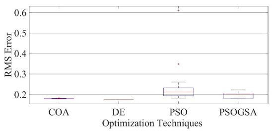
Figure A1.
Comparison between RMSE using COA and other techniques for a mono-crystalline LSM20 solar cell module (SDM).
Figure A1.
Comparison between RMSE using COA and other techniques for a mono-crystalline LSM20 solar cell module (SDM).
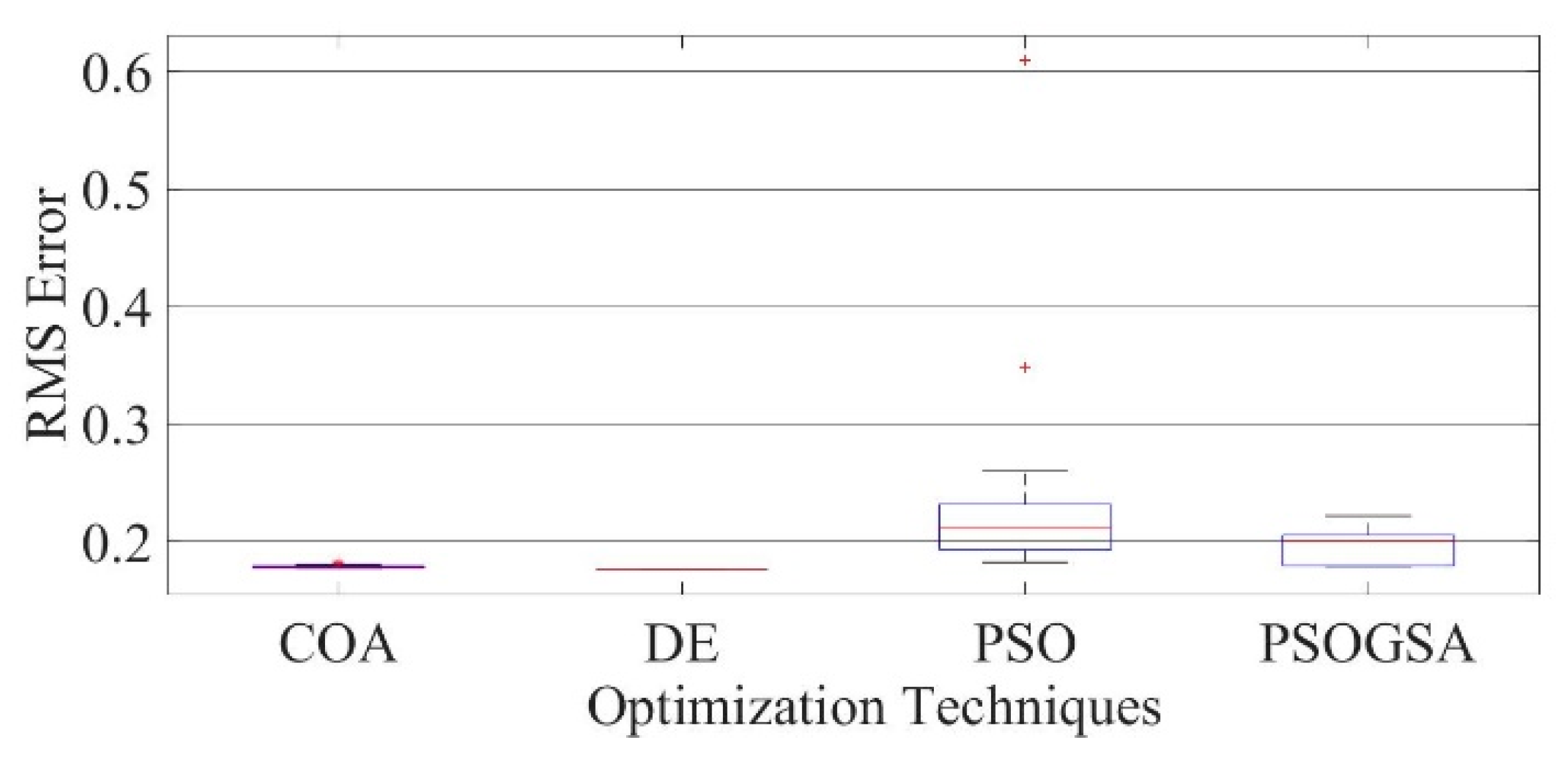
The RMSE values for the Photowatt-PWP201 module and GaAs thin-film solar cell-PVM752 (single diode model) are also compared using boxplot by different techniques, as shown in Figure A2 and Figure A3, respectively.
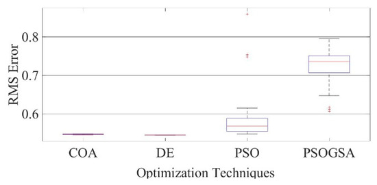
Figure A2.
Comparison between RMSE using COA and other techniques for Photowatt-PWP201 solar cell module (SDM).
Figure A2.
Comparison between RMSE using COA and other techniques for Photowatt-PWP201 solar cell module (SDM).


Figure A3.
Comparison between RMSE using COA and other techniques for GaAs thin-film solar cell (SDM).
Figure A3.
Comparison between RMSE using COA and other techniques for GaAs thin-film solar cell (SDM).
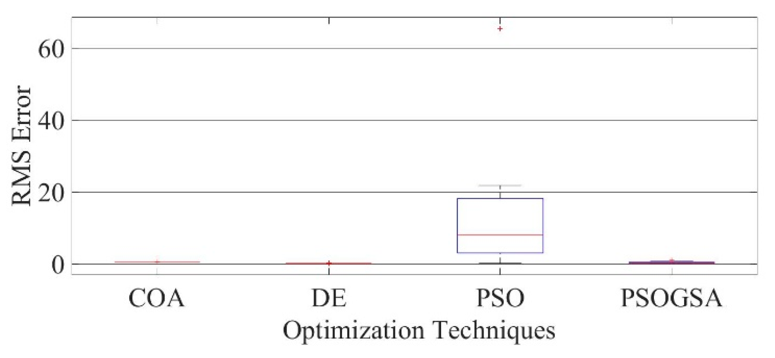
For the LSM20 solar cell module (double diode model), RMSE for various measurement techniques is illustrated in Figure A4 using a boxplot.
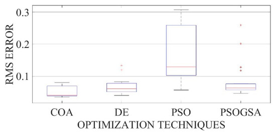
Figure A4.
Comparison between RMSE using COA and other techniques for a mono-crystalline LSM20 solar cell module (DDM).
Figure A4.
Comparison between RMSE using COA and other techniques for a mono-crystalline LSM20 solar cell module (DDM).
The RMSE values for the Photowatt-PWP201 module and GaAs thin-film solar cell-PVM752 (double diode model) are also compared using a boxplot by different techniques, as shown in Figure A5 and Figure A6, respectively.
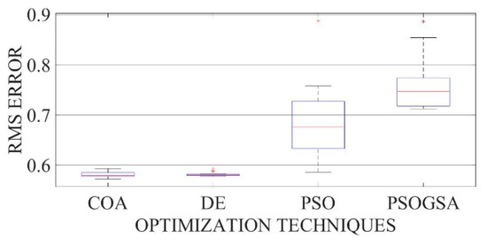
Figure A5.
Comparison between RMSE using COA and other techniques for Photowatt-PWP201 solar cell module (DDM).
Figure A5.
Comparison between RMSE using COA and other techniques for Photowatt-PWP201 solar cell module (DDM).

Figure A6.
I–V curves for the experimentally measured data and the estimated results for GaAs thin-film solar cell (DDM).
Figure A6.
I–V curves for the experimentally measured data and the estimated results for GaAs thin-film solar cell (DDM).
For the LSM20 solar cell module (three diode model), RMSE for various measurement techniques is illustrated in Figure A7 using a boxplot.
Figure A7.
Comparison between RMSE using COA and other techniques for a mono-crystalline LSM20 solar cell module (TDM).
Figure A7.
Comparison between RMSE using COA and other techniques for a mono-crystalline LSM20 solar cell module (TDM).
The RMSE values for the Photowatt-PWP201 module and GaAs thin-film solar cell-PVM752 (three diode model) are also compared using a boxplot with different techniques, as shown in Figure A8 and Figure A9, respectively.
Figure A8.
Comparison between RMSE using COA and other techniques for Photowatt-PWP201 solar cell module (TDM).
Figure A8.
Comparison between RMSE using COA and other techniques for Photowatt-PWP201 solar cell module (TDM).
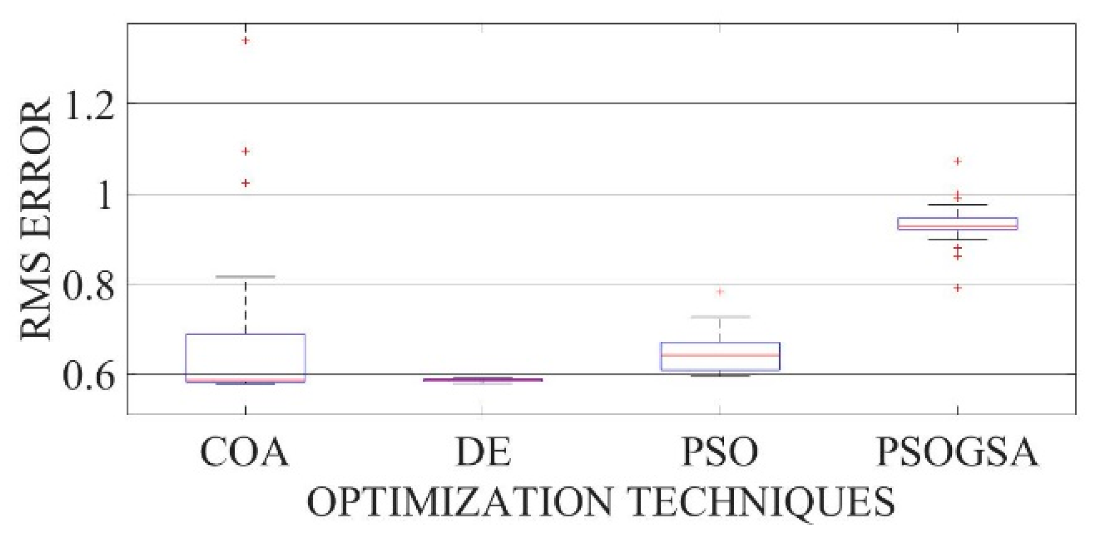
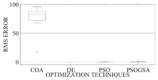
Figure A9.
Comparison between RMSE using COA and other techniques for GaAs thin-film solar cell (TDM).
Figure A9.
Comparison between RMSE using COA and other techniques for GaAs thin-film solar cell (TDM).

Appendix B
Comparison of various parameters of double diode model and three diode model for COA (without chaotic maps) and other parameter estimation techniques.
The extracted parameters are shown in Table A1, Table A2 and Table A3, for the double diode model (DDM) of mono-crystalline LSM20 module, Photowatt-PWP201 module, and PVM752, respectively, and it can be observed that COA shows a much better estimation of parameters.
Table A1.
Parameters extracted for a mono-crystalline LSM20 solar PV module by COA and its comparison with other techniques for DDM.
Table A1.
Parameters extracted for a mono-crystalline LSM20 solar PV module by COA and its comparison with other techniques for DDM.
| Parameters | COA | DE | PSO | PSOGSA |
|---|---|---|---|---|
| Rs | 0.05 | 0.05 | 0.05 | 0.05 |
| Rsh | 140.498 | 999.987 | 1000 | 689.6236 |
| IL | 0.15017 | 0.1563 | 0.159019 | 0.1608 |
| I01 | 0 | 0 | 0 | 0 |
| I02 | 0 | 0.0003 | 0.3879 | 1.3719 |
| n1 | 0.60272 | 1.510 | 4.381 | 1 |
| n2 | 0.49903 | 1.123 | 1.7654 | 2 |
| RMSE | 0.04083 | 0.04655 | 0.6169 | 0.048612 |
| Time (sec.) | 2.5570 | 1.012 | 0.9699 | 7.029 |
Table A2.
Parameters extracted for a Photowatt-PWP201 solar PV module by COA compared with other techniques for DDM.
Table A2.
Parameters extracted for a Photowatt-PWP201 solar PV module by COA compared with other techniques for DDM.
| Parameters | COA | DE | PSO | PSOGSA |
|---|---|---|---|---|
| Rs | 0.05 | 0.05 | 0.05 | 0.05 |
| Rsh | 0.6614 | 0.6549 | 0.66173 | 999.987 |
| IL | 1.16773 | 1.1716 | 1.16692 | 0.7555 |
| I01 | 5 | 3 | 5 | 3.8744 |
| I02 | 5 | 3 | 2.2291 | 3.2104 |
| n1 | 1.96225 | 1.8770 | 2.1457 | 1.7894 |
| n2 | 1.96225 | 1.8770 | 1.7413 | 1.7894 |
| RMSE | 0.5675 | 0.5856 | 0.7268 | 0.7128 |
| Time (sec.) | 2.6330 | 1.146 | 1.040 | 11.650 |
Table A3.
Parameters extracted for PVM752 GaAs thin-film solar PV cell by COA compared with other techniques for DDM.
Table A3.
Parameters extracted for PVM752 GaAs thin-film solar PV cell by COA compared with other techniques for DDM.
| Parameters | COA | DE | PSO | PSOGSA |
|---|---|---|---|---|
| Rs | 1 | 0.05 | 0.0469 | 0.0554 |
| Rsh | 1000 | 13.662 | 1000 | 998.6647 |
| IL | 0.12291 | 0.1316 | 0.1228 | 0.1118 |
| I01 | 0 | 0 | 0.002 | 0.0001 |
| I02 | 0.01216 | 0 | 0.012 | 0 |
| n1 | 2.92677 | 2 | 0.4085 | 1.8807 |
| n2 | 2.39519 | 1.781 | 0.34401 | 1.0829 |
| RMSE | 0.04005 | 0.14569 | 0.21708 | 33.3819 |
| Time (sec.) | 2.39 | 1.027 | 1.2265 | 11.977 |
The extracted parameters are shown in Table A4, Table A5 and Table A6 for the three diode model (TDM) of mono-crystalline LSM20 module, Photowatt-PWP201 module, and PVM752, respectively, and it can be observed that COA shows a much better estimation of parameters.
Table A4.
Parameters extracted for a mono-crystalline LSM20 solar PV module by COA and its comparison with other techniques for TDM.
Table A4.
Parameters extracted for a mono-crystalline LSM20 solar PV module by COA and its comparison with other techniques for TDM.
| Parameters | COA | DE | PSO | PSOGSA |
|---|---|---|---|---|
| Rs | 0.05 | 0.05 | 0.05 | 0.9745 |
| Rsh | 902.3729 | 940.92 | 1000 | 863.6476 |
| IL | 0.151626 | 0.1536 | 0.16504 | 0.1406 |
| I01 | 9 × 10⁻⁴ | 0 | 0.002803 | 4.4411 |
| I02 | 0 | 0.0054 | 0.000050 | 1.9226 |
| I03 | 0 | 0.0887 | 0.005 | 1.4669 |
| n1 | 0.74364 | 0.9445 | 5 | 2.7619 |
| n2 | 2 | 3.8352 | 1.115 | 4.9773 |
| n3 | 1.67313 | 3.4296 | 5 | 2.7642 |
| RMSE | 0.03192 | 0.0478 | 0.053484 | 0.13897 |
| Time (sec.) | 2.420 | 1.0980 | 1.54 | 14.08 |
Table A5.
Parameters extracted for a Photowatt-PWP201 solar PV module by COA compared with other techniques for TDM.
Table A5.
Parameters extracted for a Photowatt-PWP201 solar PV module by COA compared with other techniques for TDM.
| Parameters | COA | DE | PSO | PSOGSA |
|---|---|---|---|---|
| Rs | 0.05 | 0.05 | 0.05 | 0.3571 |
| Rsh | 0.66614 | 0.6640 | 0.664016 | 629.6271 |
| IL | 1.17658 | 1.1694 | 1.16924 | 0.8324 |
| I01 | 2.02460 | 5 | 5 | 3.5722 |
| I02 | 4.31185 | 5 | 5 | 2.6484 |
| I03 | 4.21045 | 4.0206 | 2.8013 | 0.4331 |
| n1 | 2 | 2.0939 | 2.0939 | 2.8021 |
| n2 | 2 | 2.0939 | 2.0939 | 2.6180 |
| n3 | 2 | 4.6802 | 5 | 2.6855 |
| RMSE | 0.58053 | 0.5675 | 0.60298 | 0.92678 |
| Time (sec.) | 2.230 | 1.321 | 1.437 | 14.518 |
Table A6.
Parameters extracted for PVM752 GaAs thin-film solar PV cell by COA compared to other techniques for TDM.
Table A6.
Parameters extracted for PVM752 GaAs thin-film solar PV cell by COA compared to other techniques for TDM.
| Parameters | COA | DE | PSO | PSOGSA |
|---|---|---|---|---|
| Rs | 1 | 1 | 0.05 | 0.2001 |
| Rsh | 1000 | 1000 | 1000 | 743.355 |
| IL | 0.1197 | 0.1266 | 0.12654 | 0.1532 |
| I01 | 0.00049 | 0.0122 | 0.005 | 4.9820 |
| I02 | 0 | 0 | 0.0049 | 2.8344 |
| I03 | 0 | 2.9404 | 0.00025 | 4.3603 |
| n1 | 2 | 2.3952 | 4.1086 | 4.9048 |
| n2 | 0.5142 | 4.0086 | 4.1086 | 3.9848 |
| n3 | 2 | 4.9094 | 5 | 3.8023 |
| RMSE | 0.02594 | 0.046074 | 0.0532 | 0.0821 |
| Time (sec.) | 2.286 | 1.258 | 1.457 | 13.719 |
References
- Sen, S.; Ganguly, S. Opportunities, barriers and issues with renewable energy development—A discussion. Renew. Sustain. Energy Rev. 2017, 69, 1170–1181. [Google Scholar] [CrossRef]
- Tran, T.; Smith, A. Evaluation of renewable energy technologies and their potential for technical integration and cost-effective use within the U.S. energy sector. Renew. Sustain. Energy Rev. 2017, 80, 1372–1388. [Google Scholar] [CrossRef]
- Rashid, K.; Safdarnejad, S.M.; Powell, K.M. Dynamic simulation, control, and performance evaluation of a synergistic solar and natural gas hybrid power plant. Energy Convers. Manag. 2019, 179, 270–285. [Google Scholar] [CrossRef]
- Karatepe, E.; Boztepe, M.; Çolak, M. Development of a suitable model for characterizing photovoltaic arrays with shaded solar cells. Sol. Energy 2007, 81, 977–992. [Google Scholar] [CrossRef]
- Fathabadi, H. Novel neural-analytical method for determining silicon/plastic solar cells and modules characteristics. Energy Convers. Manag. 2013, 76, 253–259. [Google Scholar] [CrossRef]
- Mares, O.; Paulescu, M.; Badescu, V. A simple but accurate procedure for solving the five-parameter model. Energy Convers. Manag. 2015, 105, 139–148. [Google Scholar] [CrossRef]
- Pelap, F.; Dongo, P.; Kapim, A. Optimization of the characteristics of the PV cells using nonlinear electronic components. Sustain. Energy Technol. Assess. 2016, 16, 84–92. [Google Scholar] [CrossRef]
- Maghami, M.; Hizam, H.; Gomes, C.; Radzi, M.; Rezadad, M.; Hajighorbani, S. Power loss due to soiling on solar panel: A review. Renew. Sustain. Energy Rev. 2016, 59, 1307–1316. [Google Scholar] [CrossRef] [Green Version]
- Fouad, M.; Shihata, L.; Morgan, E. An integrated review of factors influencing the perfomance of photovoltaic panels. Renew. Sustain. Energy Rev. 2017, 80, 1499–1511. [Google Scholar] [CrossRef]
- Rashid, K. Design, Economics, and Real-Time Optimization of a Solar/Natural Gas Hybrid Power Plant. Ph.D. Thesis, The University of Utah, Salt Lake City, UT, USA, 2019. [Google Scholar]
- Orioli, A.; di Gangi, A. A procedure to calculate the five-parameter model of crystalline silicon photovoltaic modules on the basis of the tabular performance data. Appl. Energy 2013, 102, 1160–1177. [Google Scholar] [CrossRef]
- Siddiqui, M.; Abido, M. Parameter estimation for five- and seven-parameter photovoltaic electrical models using evolutionary algorithms. Appl. Soft Comput. 2013, 13, 4608–4621. [Google Scholar] [CrossRef]
- Oliva, D.; Elaziz, M.A.; Elsheikh, A.H.; Ewees, A.A. A review on meta-heuristics methods for estimating parameters of solar cells. J. Power Sources 2019, 435, 126683. [Google Scholar] [CrossRef]
- Khanna, V.; Das, B.K.; Bisht, D.; Singh, P.K. A three diode model for industrial solar cells and estimation of solar cell parameters using PSO algorithm. Renew. Energy 2015, 78, 105–113. [Google Scholar] [CrossRef]
- Luque, A.; Hegedus, S. Handbook of Photovoltaic Science and Engineering, 2nd ed.; Wiley: London, UK, 2011. [Google Scholar]
- Castaner, L.; Silvestre, S. Modelling Photovoltaic Systems Using PSpice; Wiley: London, UK, 2002. [Google Scholar]
- Nishioka, K.; Sakitani, N.; Uraoka, Y.; Fuyuki, T. Analysis of multicrystalline silicon solar cells by modified 3-diode equivalent circuit model taking leakage current through periphery into consideration. Sol. Energy Mater. Sol. Cells 2007, 91, 1222–1227. [Google Scholar] [CrossRef]
- Easwarakhanthan, T.; Bottin, J.; Bouhouch, I.; Boutrit, C. Nonlinear Minimization Algorithm for Determining the Solar Cell Parameters with Microcomputers. Int. J. Sol. Energy 1986, 4, 1–12. [Google Scholar] [CrossRef]
- Chan, D.; Phillips, J.; Phang, J. A comparative study of extraction methods for solar cell model parameters. Solid-State Electron. 1986, 29, 329–337. [Google Scholar] [CrossRef]
- Ortizconde, A.; Garciasanchez, F.; Muci, J. New method to extract the model parameters of solar cells from the explicit analytic solutions of their illuminated characteristics. Sol. Energy Mater. Sol. Cells 2006, 90, 352–361. [Google Scholar] [CrossRef]
- Nassar-eddine, I.; Obbadi, A.; Errami, Y.; El fajri, A.; Agunaou, M. Parameter estimation of photovoltaic modules using iterative method and the Lambert W function: A comparative study. Energy Convers. Manag. 2016, 119, 37–48. [Google Scholar] [CrossRef]
- Gao, X.; Cui, Y.; Hu, J.; Xu, G.; Yu, Y. Lambert W-function based exact representation for double diode model of solar cells: Comparison on fitness and parameter extraction. Energy Convers. Manag. 2016, 127, 443–460. [Google Scholar] [CrossRef]
- Peng, L.; Sun, Y.; Meng, Z. An improved model and parameters extraction for photovoltaic cells using only three state points at standard test condition. J. Power Sources 2014, 248, 621–631. [Google Scholar] [CrossRef]
- Cubas, J.; Pindado, S.; de Manuel, C. Explicit Expressions for Solar Panel Equivalent Circuit Parameters Based on Analytical Formulation and the Lambert W-Function. Energies 2014, 7, 4098–4115. [Google Scholar] [CrossRef] [Green Version]
- Lim, L.; Ye, Z.; Ye, J.; Yang, D.; Du, H. A Linear Identification of Diode Models from Single I–V Characteristics of PV Panels. IEEE Trans. Ind. Electron. 2015, 62, 4181–4193. [Google Scholar] [CrossRef] [Green Version]
- Lim, L.; Ye, Z.; Ye, J.; Yang, D.; Du, H. A linear method to extract diode model parameters of solar panels from a single I–V curve. Renew. Energy 2015, 76, 135–142. [Google Scholar] [CrossRef] [Green Version]
- Tsuno, Y.; Hishikawa, Y.; Kurokawa, K. Modeling of the I–V curves of the PV modules using linear interpolation/extrapolation. Sol. Energy Mater. Sol. Cells 2009, 93, 1070–1073. [Google Scholar] [CrossRef] [Green Version]
- Lun, S.; Du, C.; Guo, T.; Wang, S.; Sang, J.; Li, J. A new explicit I–V model of a solar cell based on Taylor’s series expansion. Sol. Energy 2013, 94, 221–232. [Google Scholar] [CrossRef]
- Lun, S.; Guo, T.; Du, C. A new explicit I–V model of a silicon solar cell based on Chebyshev Polynomials. Sol. Energy 2015, 119, 179–194. [Google Scholar] [CrossRef]
- Lun, S.X.; Du, C.J.; Yang, G.H.; Wang, S.; Guo, T.T.; Sang, J.S.; Li, J.P. An explicit approximate I–V characteristic model of a solar cell based on padé approximants. Sol. Energy 2013, 92, 147–159. [Google Scholar] [CrossRef]
- Lun, S.; Du, C.; Sang, J.; Guo, T.; Wang, S.; Yang, G. An improved explicit I–V model of a solar cell based on symbolic function and manufacturer’s datasheet. Sol. Energy 2014, 110, 603–614. [Google Scholar] [CrossRef]
- Zhang, Y.; Gao, S.; Gu, T. Prediction of I–V characteristics for a PV panel by combining single diode model and explicit analytical model. Sol. Energy 2017, 144, 349–355. [Google Scholar] [CrossRef]
- Alam, D.; Yousri, D.; Eteiba, M. Flower Pollination Algorithm based solar PV parameter estimation. Energy Convers. Manag. 2015, 101, 410–422. [Google Scholar] [CrossRef]
- Louzazni, M.; Khouya, A.; Amechnoue, K.; Gandelli, A.; Mussetta, M.; Crăciunescu, A. Metaheuristic Algorithm for Photovoltaic Parameters: Comparative Study and Prediction with a Firefly Algorithm. Appl. Sci. 2018, 8, 339. [Google Scholar] [CrossRef] [Green Version]
- El-Naggar, K.; AlRashidi, M.; AlHajri, M.; Al-Othman, A. Simulated Annealing algorithm for photovoltaic parameters identification. Sol. Energy 2012, 86, 266–274. [Google Scholar] [CrossRef]
- Ye, M.; Wang, X.; Xu, Y. Parameter extraction of solar cells using particle swarm optimization. J. Appl. Phys. 2009, 105, 094502. [Google Scholar] [CrossRef]
- Mughal, M.; Ma, Q.; Xiao, C. Photovoltaic Cell Parameter Estimation Using Hybrid Particle Swarm Optimization and Simulated Annealing. Energies 2017, 10, 1213. [Google Scholar] [CrossRef] [Green Version]
- Ishaque, K.; Salam, Z. An improved modeling method to determine the model parameters of photovoltaic (PV) modules using differential evolution (DE). Sol. Energy 2011, 85, 2349–2359. [Google Scholar] [CrossRef]
- Mirjalili, S.; Hashim, S.Z.M. A New Hybrid PSOGSA Algorithm for Function Optimization. In Proceedings of the International Conference on Computer and Information Application, Bali Island, Indonesia, 19–21 March 2010. [Google Scholar]
- Yang, X.-S. Nature-Inspired Metaheuristic Algorithms; Luniver Press: Frome, UK, 2010. [Google Scholar]
- Yang, X. Multiobjective firefly algorithm for continuous optimization. Eng. Comput. 2012, 29, 175–184. [Google Scholar] [CrossRef] [Green Version]
- Yang, X.-S.; He, X.-S. Why the Firefly Algorithm Works? In Nature-Inspired Algorithms and Applied Optimization; Springer: Cham, Switzerland, 2018; pp. 245–259. [Google Scholar]
- Yang, X.-S. Engineering Optimization: An Introduction with Metaheuristic Applications; Wiley: Hoboken, NJ, USA, 2010. [Google Scholar]
- Fister, I.; Fister, I.; Yang, X.; Brest, J. A comprehensive review of firefly algorithms. Swarm Evol. Comput. 2013, 13, 34–46. [Google Scholar] [CrossRef] [Green Version]
- Kirkpatrick, S.; Gelatt, C.; Vecchi, M. Optimization by Simulated Annealing. Science 1983, 220, 671–680. [Google Scholar] [CrossRef] [PubMed]
- Pierezan, J.; Coelho, L.D.S. Coyote Optimization Algorithm: A new Metaheuristic for global optimization problems. In Proceedings of the IEEE Congress on Evolutionary Computation (CEC), Rio de Janeiro, Brazil, 1–8 July 2018. [Google Scholar]
- Qais, M.; Hasanien, H.; Alghuwainem, S.; Nouh, A. Coyote optimization algorithm for parameters extraction of three-diode photovoltaic models of photovoltaic modules. Energy 2019, 187, 116001. [Google Scholar] [CrossRef]
- Chin, V.; Salam, Z. Coyote optimization algorithm for the parameter extraction of photovoltaic cells. Sol. Energy 2019, 194, 656–670. [Google Scholar] [CrossRef]
- Pourmousaa, N.; Ebrahimib, S.M.; Malekzadehb, M.; Alizadeh, M. Parameter estimation of photovoltaic cells using improved Lozi map based chaotic optimization Algorithm. Sol. Energy 2019, 180, 180–191. [Google Scholar] [CrossRef]
- Diab, A.; Sultan, H.; Do, T.; Kamel, O.; Mossa, M. Coyote Optimization Algorithm for Parameters Estimation of Various Models of Solar Cells and PV Modules. IEEE Access 2020, 8, 111102–111140. [Google Scholar] [CrossRef]
- Muhammad, F.; Sangawi, A.K.; Hashim, S.; Ghoshal, S.; Abdullah, I.; Hameed, S. Simple and efficient estimation of photovoltaic cells and modules parameters using approximation and correction technique. PLoS ONE 2019, 14, e0216201. [Google Scholar] [CrossRef] [PubMed] [Green Version]
- Saremi, S.; Mirjalili, S.; Lewis, A. Biogeography-based optimisation with chaos. Neural Comput. Appl. 2014, 25, 1077–1097. [Google Scholar] [CrossRef]
- Wang, N.; Liu, L.; Liu, L. Genetic algorithm in chaos. OR Trans. 2001, 5, 1–10. [Google Scholar]
- Li-Jiang, Y.; Tian-Lun, C. Application of Chaos in Genetic Algorithms. Commun. Theor. Phys. 2002, 38, 168–172. [Google Scholar] [CrossRef]
- Jothiprakash, V.; Arunkumar, R. Optimization of Hydropower Reservoir Using Evolutionary Algorithms Coupled with Chaos. Water Resour. Manag. 2013, 27, 1963–1979. [Google Scholar] [CrossRef]
- Zhenyu, G.; Bo, C.; Min, Y.; Binggang, C. Self-adaptive chaos differential evolution. In Advances in Natural Computation. Lecture notes in Computer Science; Springer: Berlin/Heidelberg, Germany, 2006; Volume 4221, pp. 972–975. [Google Scholar]
- Saremi, S.; Mirjalili, S.; Mirjalili, S. Chaotic Krill Herd Optimization Algorithm. Procedia Technol. 2014, 12, 180–185. [Google Scholar] [CrossRef]
- Wang, G.; Guo, L.; Gandomi, A.; Hao, G.; Wang, H. Chaotic Krill Herd algorithm. Inf. Sci. 2014, 274, 17–34. [Google Scholar] [CrossRef]
- Simon, D. Biogeography-Based Optimization. IEEE Trans. Evol. Comput. 2008, 12, 702–713. [Google Scholar] [CrossRef] [Green Version]
- Du, D.; Simon, D.; Ergezer, M. Biogeography-based optimization combined with evolutionary strategy and immigration refusal. In Proceedings of the IEEE International Conference on Systems, Man and Cybernetics, San Antonio, TX, USA, 11–14 October 2009; pp. 997–1002. [Google Scholar]
- Bhattacharya, A.; Chattopadhyay, P. Hybrid Differential Evolution with Biogeography-Based Optimization for Solution of Economic Load Dispatch. IEEE Trans. Power Syst. 2010, 25, 1955–1964. [Google Scholar] [CrossRef]
- Kiani, A.T.; Nadeem, M.F.; Ahmed, A.; Sajjad, I.A.; Raza, A.; Khan, I.A. Chaotic Inertia Weight Particle Swarm Optimization (CIWPSO): An Efficient Technique for Solar Cell Parameter Estimation. In Proceedings of the 2020 3rd International Conference on Computing, Mathematics and Engineering Technologies (iCoMET), Sindh, Pakistan, 29–30 January 2020; pp. 1–6. [Google Scholar]
- Kiani, A.T.; Nadeem, M.F.; Ahmed, A.; Khan, I.; Elavarasan, R.M.; Das, N. Optimal PV Parameter Estimation via Double Exponential Function-Based Dynamic Inertia Weight Particle Swarm Optimization. Energies 2020, 13, 4037. [Google Scholar] [CrossRef]
- Ahmad, I.; Arif, M.S.; Cheema, I.I.; Thollander, P.; Khan, M.A. Drivers and Barriers for Efficient Energy Management Practices in Energy-Intensive Industries: A Case-Study of Iron and Steel Sector. Sustainability 2020, 12, 7703. [Google Scholar] [CrossRef]
- Beig, B.; Niazi, M.B.K.; Jahan, Z.; Pervaiz, E.; Shah, G.A.; Haq, M.U.; Zafar, M.I.; Zia, M. Slow-Release Urea Prills Developed Using Organic and Inorganic Blends in Fluidized Bed Coater and Their Effect on Spinach Productivity. Sustainability 2020, 12, 5944. [Google Scholar] [CrossRef]
- Razzaq, L.; Farooq, M.; Mujtaba, M.A.; Sher, F.; Farhan, M.; Hassan, M.T.; Soudagar, M.E.M.; Atabani, A.E.; Kalam, M.A.; Imran, M. Modeling Viscosity and Density of Ethanol-Diesel-Biodiesel Ternary Blends for Sustainable Environment. Sustainability 2020, 12, 5186. [Google Scholar] [CrossRef]
- Talip, R.A.A.; Yahya, W.Z.N.; Bustam, M.A. Ionic Liquids Roles and Perspectives in Electrolyte for Dye-Sensitized Solar Cells. Sustainability 2020, 12, 7598. [Google Scholar] [CrossRef]
- Lu, Y.; Khan, Z.A.; Alvarez-Alvarado, M.S.; Zhang, Y.; Huang, Z.; Imran, M. A Critical Review of Sustainable Energy Policies for the Promotion of Renewable Energy Sources. Sustainability 2020, 12, 5078. [Google Scholar] [CrossRef]


Publisher’s Note: MDPI stays neutral with regard to jurisdictional claims in published maps and institutional affiliations. |
© 2021 by the authors. Licensee MDPI, Basel, Switzerland. This article is an open access article distributed under the terms and conditions of the Creative Commons Attribution (CC BY) license (https://creativecommons.org/licenses/by/4.0/).