Adaptive Sparse Representation of Continuous Input for Tsetlin Machines Based on Stochastic Searching on the Line

Abstract

This paper introduces a novel approach to representing continuous inputs in Tsetlin Machines (TMs). Instead of using one Tsetlin Automaton (TA) for every unique threshold found when Booleanizing continuous input, we employ two Stochastic Searching on the Line (SSL) automata to learn discriminative lower and upper bounds. The two resulting Boolean features are adapted to the rest of the clause by equipping each clause with its own team of SSLs, which update the bounds during the learning process. Two standard TAs finally decide whether to include the resulting features as part of the clause. In this way, only four automata altogether represent one continuous feature (instead of potentially hundreds of them). We evaluate the performance of the new scheme empirically using five datasets, along with a study of interpretability. On average, TMs with SSL feature representation use $4.3$ times fewer literals than the TM with static threshold-based features. Furthermore, in terms of average memory usage and F1-Score, our approach outperforms simple Multi-Layered Artificial Neural Networks, Decision Trees, Support Vector Machines, K-Nearest Neighbor, Random Forest, Gradient Boosted Trees (XGBoost), and Explainable Boosting Machines (EBMs), as well as the standard and real-value weighted TMs. Our approach further outperforms Neural Additive Models on Fraud Detection and StructureBoost on CA-58 in terms of the Area Under Curve while performing competitively on COMPAS.

1. Introduction

Deep learning (DL) has significantly advanced state-of-the-art models in machine learning (ML) over the last decade, attaining remarkable accuracy in many ML application domains. One of the issues with DL, however, is that DL inference cannot easily be interpreted [1]. This limits the applicability of DL in high-stakes domains such as medicine [2,3], credit-scoring [4,5], churn prediction [6,7], bioinformatics [8,9], crisis analysis [10], and criminal justice [11]. In this regard, the simpler and more interpretable ML algorithms, such as Decision Trees, Logistic Regression, Linear Regression, and Decision Rules, can be particularly suitable. However, they are all hampered by low accuracy when facing complex problems [12]. This limitation has urged researchers to develop machine learning algorithms that are capable of achieving a better trade-off between interpretability and accuracy.

While some researchers focus on developing entirely new machine learning algorithms, as discussed above, other researchers try to render DL interpretable. A recent attempt to make DL interpretable is the work of Agarwal et al. [11]. They introduce Neural Additive Models (NAMs), which treat each feature independently. The assumption of independence makes NAMs interpretable but impedes accuracy compared with regular DL [11]. Another approach is to try to explain DL inference with surrogate models. Here, one strives to attain local interpretability; i.e., explaining individual predictions [13]. Nevertheless, these explanations are only approximate and cannot explain the complete DL model (global interpretability) [14].

Many prominent interpretable ML approaches are based on natively interpretable rules, tracing back to some of the well-known learning models such as association rule learning [15]. These have for instance been used to predict sequential events [16]. Other examples include the work of Feldman on the difficulty of learning formulae in Disjunctive Normal Form (DNF) [17] and Probably Approximately Correct (PAC) learning, which has provided fundamental insights into machine learning as well as a framework for learning formulae in DNF [18]. Approximate Bayesian techniques are another set of approaches for the robust learning of rules [19,20]. Hybrid Logistic Circuits (HLC), introduced in [21], are yet another novel approach to interpretable machine learning. Here, layered logical operators translate into a logistic regression function. HLC has demonstrated promising accuracy in image classification. However, in general, rule-based machine learning scales poorly and is prone to noise. Indeed, for data-rich problems, in particular those involving natural language and sensory inputs, rule-based machine learning is inferior to DL.

Another recent interpretable approach to machine learning is Explainable Boosting Machines (EBMs) [22]. EBMs are highly intelligible and explainable, while their accuracy is comparable to state-of-the-art machine learning methods such as Random Forest and Boosted Trees [23]. Indeed, EBMs are recognized as state-of-the-art within Generalized Additive Models (GAMs) [22,23]. The EBMs learn feature functions independently, using methods such as gradient boosting or bagging. This allows the user to determine how much each feature contributes to the model’s prediction and is hence directly interpretable.

Despite being rule-based, the recently introduced Tsetlin Machines (TMs) [24] have obtained competitive accuracy in a wide range of domains [25,26,27,28,29], while producing human-interpretable outputs. At the same time, TMs utilize comparably low computational resources [30]. Employing a team of TAs [31], a TM learns a linear combination of conjunctive clauses in propositional logic, producing decision rules similar to the branches in a decision tree (e.g., if X satisfies condition A and not condition B then Y = 1) [26]. In other words, the TM can be said to unify logistic regression and rule-based learning in a way that boosts accuracy while maintaining interpretability.

Regarding recent progress on TMs, they have recently been adopted for various application domains such as natural language understanding [32,33], image classification [34], and speech processing [35]. Simultaneously, the TM architecture and learning mechanism has been improved in terms of accuracy, computation speed, and energy usage. The convolutional TM provides competitive performance on MNIST, Fashion-MNIST, and Kuzushiji-MNIST, in comparison with CNNs, K-Nearest Neighbor, Support Vector Machines, Random Forests, Gradient Boosting, Binary Connect, Logistic Circuits, and ResNet [36]. The regression TM [27] opens up for continuous output, achieving on par or better performance compared to Random Forest, Regression Trees, and Support Vector Regression. With the proposed Booleanization scheme in [37], the TM is also able to operate with continuous features.

Furthermore, clauses are enhanced with weights in [25]. The weights reduce the number of clauses required without any loss of accuracy. Later, integer weights replaced real-valued weights to both reduce the number of clauses and to increase the interpretability of the TM [38]. On several benchmarks, the integer-weighted TM version outperformed simple Multi-Layered Artificial Neural Networks, Support Vector Machines, Decision Trees, Random Forest, K-Nearest Neighbor, Random Forest, Explainable Boosting Machines (EBMs), and Gradient Boosted Trees (XGBoost), as well as the standard TM. Further, the introduced multi-granular clauses for TM in [28] eliminate the pattern specificity parameter from the TM, consequently simplifying the hyper-parameter search. By indexing the clauses on the features that falsify them, up to an order of magnitude faster inference and learning has been reported [29]. Several researchers have further introduced techniques and architectures that reduce memory footprint and energy usage [39], while other techniques improve learning speed [39,40] and support explainability [41,42].

Recent theoretical work proves the convergence to the correct operator for “identity” and “not”. It is further shown that arbitrarily rare patterns can be recognized using a quasi-stationary Markov chain-based analysis. The work finally proves that when two patterns are incompatible, the most accurate pattern is selected [43]. Convergence for the “XOR” operator has also recently been proven by Jiao et al. [44].

The approach proposed in [37] is currently the most effective way of representing continuous features through Booleanization. However, the approach requires a large number of TAs to represent the Booleanized continuous features. Indeed, one TA is needed per unique continuous value. Consequently, this increases the training time of the TM as it needs to update all the TAs in all of clauses for each training iteration. Further, this adds more post-processing work for generating interpretable rules out of TM outputs. To overcome this challenge in TMs, we propose a novel approach to represent continuous features in the TM, encompassing the following contributions:

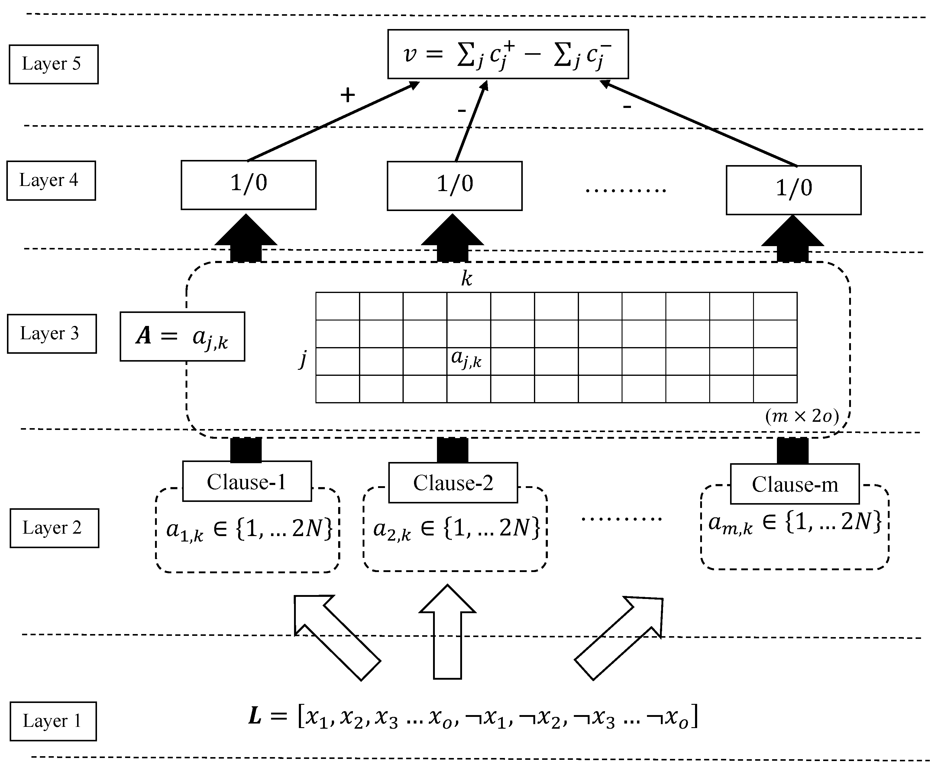
• Instead of representing each unique threshold found in the Booleanization process by a TA, we use a Stochastic Searching on the Line (SSL) automaton [45] to learn the lower and upper limits of the continuous feature values. These limits decide the Boolean representation of the continuous value inside the clause. Only two TAs then decide whether to include these bounds in the clause or to exclude them from the clause. In this way, one continuous feature can be represented by only four automata, instead of representing it by hundreds of TAs (decided by the number of unique feature values within the feature).
• A new approach to calculating the clause output is introduced to match with the above Booleanization scheme.
• We update the learning procedure of the TM accordingly, building upon Type I and Type II feedback to learn the lower and upper bounds of the continuous input.
• Empirically, we evaluate our new scheme using eight data sets: Bankruptcy, Balance Scale, Breast Cancer, Liver Disorders, Heart Disease, Fraud Detection, COMPAS, and CA-58. With the first five datasets, we show how our novel approach affects memory consumption, training time, and the number of literals included in clauses, in comparison with the threshold-based scheme [46]. Furthermore, performances on all these datasets are compared against recent state-of-the-art machine learning models.

This paper is organized as follows. In Section 2, we present the learning automata foundation we build upon and discuss the SSL automaton in more detail. Then, in Section 3, we introduce the TM and how it traditionally has dealt with continuous features. We then propose our new SSL-based scheme. We evaluate the performance of our new scheme empirically using five datasets in Section 5. In this section, we use the Bankruptcy dataset to demonstrate how rules are extracted from TM clause outputs. The prediction accuracy of the TM SSL-based continuous feature representation is then compared against several competing techniques, including ANNs, SVMs, DTs, RF, KNN, EBMs (the current state-of-the-art of Generalized Additive Models (GAMs) [22,23]), Gradient Boosted Trees (XGBoost), and the TM with regular continuous feature representation. Further, we contrast the performance of the TM against reported results on recent state-of-the-art machine learning models, namely NAMs [11] and StructureBoost [47]. Finally, we conclude our paper in Section 6.

2. Learning Automata and the Stochastic Searching on the Line Automaton

The origins of Learning Automata (LA) [48] can be traced back to the work of M. L. Tsetlin in the early 1960s [31]. In a stochastic environment, an automaton is capable of learning the optimum action that has the lowest penalty probability through trial and error. There are different types of automata; the choice of a specific type is decided by the nature of the application [49].

Initially, the LA randomly perform an action from an available set of actions. This action is then evaluated by its attached environment. The environment randomly produces feedback; i.e., a reward or a penalty as a response to the action selected by the LA. Depending on the feedback, the state of the LA is adjusted. If the feedback is a reward, the state changes towards the end state of the selected action, reinforcing the action. When the feedback is a penalty, the state changes towards the center state of the selected action, weakening the action and eventually switching the action. The next action of the automaton is then decided by the new state. In this manner, an LA interacts with its environment iteratively. With a sufficiently large number of states and a reasonably large number of interactions with the environment, an LA learns to choose the optimum action with a probability arbitrarily close to $1.0$ [48].

During LA learning, the automaton can make deterministic or stochastic jumps as a response to the environment feedback. LA make stochastic jumps by randomly changing states according to a given probability. If this probability is $1.0$, the state jumps are deterministic. Automata of this kind are called deterministic automata. If the transition graph of the automaton is kept static, we refer to it as a fixed-structure automaton. The TM employs TAs to decide which literals to include in the clauses. A TA is deterministic and has a fixed structure, formulated as a finite-state automaton [31]. A TA with $2N$ states is depicted in Figure 1. States 1 to N map to Action 1 and states $N+1$ to $2N$ map to Action 2.

The Stochastic Searching on the Line (SSL) automaton pioneered by Oommen [45] is somewhat different from regular automata. The SSL automaton is an optimization scheme designed to find an unknown optimum location ${\lambda }^{*}$ on a line, seeking a value between 0 to 1, $[0,1]$.

In SSL learning, ${\lambda }^{*}$ can be one of the N points. In other words, the search space is divided into N points, {$0,1/N,2/N,\dots ,(N-1)/N,1$}, with N being the discretization resolution. Depending on the possibly faulty feedback from the attached environment (E), $\lambda$ moves towards the left or right from its current state on the created discrete search space. We consider the environment feedback 1, $E=1$, as an indication to move towards right (or to increase the value of $\lambda$) by one step. The environment feedback 0, $E=0$, on the other hand, is considered as an indication to move towards the left (or to decrease the value of $\lambda$) by one step. The next location of $\lambda$, $\lambda (n+1)$ can thus be expressed as follows:

$$\lambda (n+1)=\left\{\begin{array}{cc}\lambda \left(n\right)+1/N,\hfill & \mathrm{if}E\left(n\right)=1\mathrm{and}0⩽\lambda \left(n\right)<1,\hfill \\ \lambda \left(n\right)-1/N,\hfill & \mathrm{if}E\left(n\right)=0\mathrm{and}0<\lambda \left(n\right)⩽1.\hfill \end{array}\right.$$

(1)

$$\lambda (n+1)=\left\{\begin{array}{cc}\lambda \left(n\right),\hfill & \mathrm{if}\lambda \left(n\right)=1\mathrm{and}E\left(n\right)=1,\hfill \\ \lambda \left(n\right),\hfill & \mathrm{if}\lambda \left(n\right)=0\mathrm{and}E\left(n\right)=0.\hfill \end{array}\right.$$

(2)

Asymptotically, the learning mechanism is able to find a value arbitrarily close to ${\lambda }^{*}$ when $N\to \infty$ and $n\to \infty$.

3. Tsetlin Machine (TM) for Continuous Features

As seen in Figure 2, conceptually, the TM decomposes into five layers to recognize sub-patterns in the data and categorize them into classes. In this section, we explain the job of each of these layers in the pattern recognition and learning phases of the TM. The parameters and symbols used in this section are explained and summarized in

Table 1. Parameters and symbols used in Section 3.

Parameter/Symbol	Description	Parameter/Symbol	Description
$\mathit{X}$	Input vector containing o propositional variables	$\mathit{L}$	The augmented feature set containing both original and negated features
$x_k$	$k^{th}$ propositional variable	$l_k$	$k^{th}$ literal
m	The number of clauses	$c_j$	$j^{th}$ clause and stored in vector $\mathbf{C}$
$I_j$	The index set of the included literals in clause j	N	The number of states per action in the TA
$a_{j,k}$	State of the $k^{th}$ literal in the $j^{th}$ clause, stored in matrix $\mathbf{A}$	$I_X^1$	The indexes of the literals of value 1
v	The difference between positive and negative clause outputs	$p_j$	Decision on receiving Type I or Type II feedback, stored in vector $\mathbf{P}$
T	Feedback threshold	s	Learning sensitivity
$r_{j,k}$	The decision whether the $k^{th}$ TA of the $j^{th}$ clause is to receive Type Ia feedback, stored in matrix $\mathbf{R}$	$q_{j,k}$	The decision whether the $k^{th}$ TA of the $j^{th}$ clause is to receive Type Ib feedback, stored in matrix $\mathbf{Q}$
$I^{\mathrm{Ia}}$	Stores TA indexes selected for Type Ia feedback	$I^{\mathrm{Ib}}$	Stores TA indexes selected for Type Ib feedback
⊕	Denotes adding 1 to the current state value of the TA	⊖	Denotes substracting 1 from the current state value of the TA
$I^{\mathrm{II}}$	Stores TA indexes selected for Type II feedback

.

Layer 1: the input. In the input layer, the TM receives a vector of o propositional variables: $\mathbf{X}$, $x_k\in {\{0,1\}}^o$. The objective here of the TM is to classify this feature vector into one of the two classes, $y\in \{0,1\}$. However, as shown in Figure 2, the input layer also includes negations of the original features, $\neg x_k$, in the feature set to capture more sophisticated patterns. Collectively, the elements in the augmented feature set are called literals: $\mathbf{L}=[x_1,x_2,\dots ,x_o,$ $\neg x_1,\neg x_2,\dots ,\neg x_o]=$ $[l_1,l_2,\dots ,l_{2o}]$.

Layer 2: clause construction. The sub-patterns associated with class 1 and class 0 are captured by m conjunctive clauses. The value m is set by the user where more complex problems might demand a large m. All clauses receive the same augmented feature set formulated at the input layer, $\mathbf{L}$. However, to perform the conjunction, only a fraction of the literals is utilized. The TM employs two-action TAs in Figure 1 to decide which literals are included in which clauses. Since we found a number $2\times o$ of literals in $\mathbf{L}$, the same number of TAs—one per literal k—is needed by a clause to decide the included literals in the clause. When the index set of the included literals in clause j is given in $I_j$, the conjunction of the clause can be performed as follows:

$$c_j=\underset{k\in I_j}{\bigwedge }{l}_k.$$

(3)

Notice how the composition of a clause varies from another clause depending on the indexes of the included literals in the set $I_j\subseteq \{1,\dots ,2o\}$. For the special case of $I_j=\varnothing$—i.e., an empty clause—we have

$$c_j=\left\{\begin{array}{cc}1\hfill & \mathbf{during}\mathrm{learning}\hfill \\ 0\hfill & \mathbf{otherwise}.\hfill \end{array}\right.$$

(4)

That is, during learning, empty clauses output 1, and during classification, they output 0.

Layer 3: storing states of TAs of clauses in the memory. The TA states on the left-hand side of the automaton (states from 1 to N) ask to exclude the corresponding literal from the clause while the states on the right-hand side of the automaton (states from $N+1$ to $2N$) ask to include the literal in the clause. The systematic storage of states of TAs in the matrix, $\mathbf{A}$: $\mathbf{A}=\left(a_{j,k}\right)\in {\{1,\dots ,2N\}}^{m\times 2o}$, with j referring to the clause and k to the literal, allows us to find the index set of the included literals in clause j, $I_j$ as $I_j=\left\{k\right|a_{j,k}>N,$ $1\le k\le 2o\}$.

Layer 4: clause output. Once the TA decisions are available, the clause output can be easily computed. Since the clauses are conjunctive, a single literal of value 0 is enough to turn the clause output to 0 if its corresponding TA has decided to include it in the clause. To make the understanding easier, we introduce set $I_X^1$, which contains the indexes of the literals of value 1. Then, the output of clause j can be expressed as

$$c_j=\left\{\begin{array}{cc}1\hfill & \mathrm{if}{I}_j\subseteq I_X^1,\hfill \\ 0\hfill & \mathrm{otherwise}.\hfill \end{array}\right.$$

(5)

The clause outputs, computed as above, are now stored in vector $\mathbf{C}$, i.e., $\mathbf{C}=\left(c_j\right)\in {\{0,1\}}^m$.

Layer 5: classification: The TM structure given in Figure 2 is used to classify data into two classes. Hence, sub-patterns associated with each class have to be separately learned. For this purpose, the clauses are divided into two groups, where one group learns the sub-pattern of class 1 while the other learns the sub-patterns of class 0. For simplicity, clauses with an odd index are assigned a positive polarity ($c_j^{+}$), and they are used to capture sub-patterns of output $y=1$. Clauses with an even index, on the other hand, are assigned negative polarity ($c_j^{-}$) and they seek the sub-patterns of output $y=0$.

The clauses that recognize sub-patterns output 1. This makes the classification process easier as we simply need to sum the clause outputs of each class and assign the sample into the class which has the highest sum. A higher sum means that more sub-patterns are identified from the designated class and that there is a higher chance of the sample being in that class. Hence, with v being the difference in clause output, $v={\sum }_j{c}_j^{+}-{\sum }_j{c}_j^{-}$, the output of the TM is decided as follows:

$$\widehat{y}=\left\{\begin{array}{cc}1\hfill & \mathrm{if}v\ge 0\hfill \\ 0\hfill & \mathrm{if}v<0.\hfill \end{array}\right.$$

(6)

A TM learns online, updating its internal parameters according to one training sample $(X,y)$ at a time. As we discussed, a TA team decides the clause output, and collectively, the output of all the clauses decides the TM’s output. Hence, to maximize the accuracy of the TM’s output, it is important to sensibly guide individual TAs in clauses. We achieve this with two kinds of reinforcement: Type I and Type II feedback. Type I and Type II feedback decide if the TAs in clauses receive a reward, a penalty, or inaction feedback, depending on the context of their actions. How the type of feedback is decided and how the TAs are updated according to the selected feedback type is discussed below in more details.

Type I feedback: Type I feedback has been designed to reinforce the true positive outputs of the clauses and to combat against the false negative outputs of the clauses. To reinforce the true positive output of a clause (the clause output is 1 when it has to be 1), include actions of TAs whose corresponding literal value is 1 are strengthened. However, more fine-tuned patterns can be identified by strengthening the exclude actions of TAs in the same clause whose corresponding literal value is 0. To combat the false negative outputs of the clauses (the clause output is 0 when it has to be 1), we erase the identified pattern by the clause and make it available for a new pattern. To do so, the exclude actions of TAs, regardless of their corresponding literal values, are strengthened. We now sub-divide the Type I feedback into Type Ia and Ib, where Type Ia handles the reinforcing of exclude actions while Type Ib works on reinforcing exclude actions of TAs. Together, Type Ia and Type Ib feedback force clauses to output 1. Hence, clauses with positive polarity need Type I feedback when $y=1$ and clauses with negative polarity need Type I feedback when $y=0$. To diversify the clauses, they are targeted for Type I feedback stochastically as follows:

$$p_j=\left\{\begin{array}{cc}1\hfill & \mathrm{with}\mathrm{probability}\frac{T-\max (-T,\min (T,v\left)\right)}{2T},\hfill \\ 0\hfill & \mathrm{otherwise}.\hfill \end{array}\right.$$

(7)

All clauses in each class should not learn the same sub-pattern, nor only a few subpatterns. Hence, clauses should be smartly allocated among the sub-patterns. The user set target T in (7) does this while deciding the probability of receiving Type I feedback; i.e., T number of clauses are available to learn each sub-pattern in each class. A higher T increases the robustness of learning by allocating more clauses to learn each sub-pattern. Now, T together with v decides the probability of clause j receiving Type I feedback, and accordingly, the decision $p_j$ is made. The decisions for the complete set of clauses to receive Type I feedback are organized in the vector $\mathbf{P}=\left(p_j\right)\in {\{0,1\}}^m$.

Once the clauses to receive Type I feedback are singled out as per (7), the probability of updating individual TAs in selected clauses is calculated using the user-set parameter s (s $\ge 1$), separately for Type Ia and Type Ib. According to the above probabilities, the decision whether the $k^{th}$ TA of the $j^{th}$ clause is to receive Type Ia feedback, $r_{j,k}$ or Type Ib feedback, $q_{j,k}$ is made stochastically as follows:

$$r_{j,k}=\left\{\begin{array}{cc}1\hfill & \mathrm{with}\mathrm{probability}\frac{s-1}{s},\hfill \\ 0\hfill & \mathrm{otherwise}.\hfill \end{array}\right.$$

(8)

$$q_{j,k}=\left\{\begin{array}{cc}1\hfill & \mathrm{with}\mathrm{probability}\frac{1}{s},\hfill \\ 0\hfill & \mathrm{otherwise}.\hfill \end{array}\right.$$

(9)

The above decisions are stored in the two matrices $\mathbf{R}$ and $\mathbf{Q}$, respectively; i.e., $\mathbf{R}=\left(r_{j,k}\right)\in {\{0,1\}}^{m\times 2o}$ and $\mathbf{Q}=\left(q_{j,k}\right)\in {\{0,1\}}^{m\times 2o}$. Using the complete set of conditions, TA indexes selected for Type Ia are $I^{\mathrm{Ia}}=\left\{(j,k)\right|l_k=1\wedge c_j=1\wedge p_j=1\wedge r_{j,k}=1\}.$ Similarly, TA indexes selected for Type Ib are $I^{\mathrm{Ib}}=\left\{(j,k)|(l_k=0\vee c_j=0)\wedge p_{j,y}=1\wedge q_{j,k}=1\right\}.$

The states of the identified TAs are now ready to be updated. Since Type Ia strengthens the include action of TAs, the current state should move more towards the include action direction. We denote this as ⊕, and here ⊕ adds 1 to the current state value of the TA. The Type Ib feedback, on the other hand, moves the state of the selected TA towards the exclude action direction to strengthen the exclude action of TAs. We denote this by ⊖, and here, ⊖ subtracts 1 from the current state value of the TA. Accordingly, the states of TAs in $\mathbf{A}$ are updated as $\mathbf{A}\leftarrow \left(\mathbf{A}\oplus I^{\mathrm{Ia}}\right)\ominus I^{\mathrm{Ib}}$.

Type II feedback: Type II feedback has been designed to combat the false positive output of clauses (the clause output is 1 when it has to be 0). To turn this clause output from 1 to 0, a literal value of 0 can simply be included in the clause. Clauses with a positive polarity need Type II feedback when $y=0$ and clauses with negative polarity need this when $y=1$ as they do not want to vote for the opposite class. Again, using the user-set target T, the decision for the $j^{th}$ clause is made as follows:

$$p_j=\left\{\begin{array}{cc}1\hfill & \mathrm{with}\mathrm{probability}\frac{T+\max (-T,\min (T,v\left)\right)}{2T},\hfill \\ 0\hfill & \mathrm{otherwise}.\hfill \end{array}\right.$$

(10)

The states of the TAs whose corresponding literal of value 0 in selected clauses according to (10) are now moved towards the include action direction with a probability of 1. Hence, the index set of this kind can be identified as $I^{\mathrm{II}}=\left\{(j,k)\right|l_k=0\wedge$ $c_j=1\wedge p_j=1\}.$ Accordingly, the states of TAs in $\mathbf{A}$ are updated as $\mathbf{A}\leftarrow \mathbf{A}\oplus I^{\mathrm{II}}$.

When training has been completed, the final decisions of the TAs are recorded, and the resulting clauses can be deployed for operation.

Booleanization of Continuous Features: In the TM discussed so far, the input layer accepted only Boolean features; i.e., $\mathit{X}=[x_1,x_2,x_3,\dots ,x_o]$ with $x_k,k=1,2,\dots ,o$, being 0 or 1. These features and their negations were directly fed into the clauses without any further modifications. However, continuous features in machine learning applications are more common than values of simply 1 or 0. In one of our previous papers [37], we presented a systematic procedure of transforming continuous features into Boolean features while maintaining ranking relationships among the continuous feature values.

We here summarize the previous Booleanization scheme using the example presented in [27]. As seen in

Table 2. Preprocessing of two continuous features.

Raw Feature		Thresholds
1	2	≤3.834	≤5.779	≤10.008	≤11.6	≤25.7	≤32.4	≤56.1
5.779	25.7	0	1	1	0	1	1	1
10.008	56.1	0	0	1	0	0	0	1
5.779	11.6	0	1	1	1	1	1	1
3.834	32.4	1	1	1	0	0	1	1

, we Booleanize the two continuous features listed in table column 1 and column 2.

• First, for each feature, the unique values are identified;
• The unique values are then sorted from smallest to largest;
• The sorted unique values are considered as thresholds. In the table, these values can be seen in the “Thresholds” row;
• The original feature values are then compared with identified thresholds, only from their own feature value set. If the feature value is greater than the threshold, set the corresponding Boolean variable to 0; otherwise, set it to 1;
• The above steps are repeated until all the features are converted into Boolean form.

The first feature in the first column of the table contains three unique values: 5.779, 10.008, and 3.834 (step (i)). Once they are sorted as required in step ii, we obtain 3.834, 5.779, and 10.008. Now, we consider them as thresholds: ≤3.834, ≤5.779, and ≤10.008 (step (iii)). Here, we find that each original feature in column 1 is going to represent 3 bit values. According to step iv, we now compare the original values in the first feature against its thresholds. The first feature value of $5.779$ is greater than $3.834$ (resulting in 0), equal to $5.779$ (resulting in 1), and less than $10.008$ (resulting in 1). Hence, we replace $5.779$ with 011. Similarly, $10.008$ and $3.834$ can be replaced with 001 and 111, respectively.

The conversion of the feature values for the second feature starts once all the feature values in the first feature are completed. This procedure is iterated until all the continuous values of all the continuous features have been converted to Boolean form (step (v)).

This Boolean representation of continuous features is particularly powerful as it allows the TM to reason about the ordering of the values, forming conjunctive clauses that specify rules based on thresholds, and with negated features, also rules based on intervals. This can be explained again with the following example.

The threshold ≤3.834 in the “Threshold” row stands for the continuous value $3.834$ of the first feature. Similarly, threshold ≤5.779 and ≤10.008 represent the continuous values $5.779$ and $10.008$, respectively. Consider a clause with threshold ≤5.779 included in the clause, which is the only threshold included in the clause. Then, for any input value less than or equal to ≤5.779 from that feature, the clause outputs 1. Now, consider the case of having two thresholds, ≤5.779 and ≤10.008, included in the clause. The threshold ≤5.779 still decides the clause output due to the fact that the AND of ≤5.779 and ≤10.008 threshold columns in Table 2 yields the threshold column ≤5.779. When a clause includes a negated threshold it reverses the original threshold. Consider a clause that only includeds the negation of the threshold ≤3.834. Now, the clause outputs 1 for all the values greater than ≤3.834 from that feature, as the NOT of ≤3.834 is equivalent to 3.834<.

The above explanation of the threshold selection reveals that the lowest original threshold included in the clause and the highest negated threshold included in the clause decide the upper and lower boundary of the feature values, and these thresholds are the only important thresholds for calculating the clause output. Hence, this motivates us to represent the continuous features in clauses in a new way and train the clauses accordingly as follows.

4. Sparse Representation of Continuous Features

However, the above representation of continuous values in clauses is costly as it needs two times the total number of unique values of TAs per clause. This is more severe when the dataset is large and when there is a large number of input features to be considered. Hence, we introduce SSL automata to represent the upper and lower limits of the continuous features. With the new representation, a continuous feature can be then represented by only two automata instead of having two times the number of unique values in the considered continuous feature. The new parameters and symbols used in this section are explained and summarized in

Table 3. Parameters and symbols used in Section 4.

Parameter/Symbol	Description	Parameter/Symbol	Description
${\mathit{X}}^c$	Input vector containing o continuous features	$x_k^c$	$k^{th}$ continuous feature
$SS{L}_{j,k}^l$	Lower limit of the continuous feature k in clause j	$SS{L}_{j,k}^u$	Upper limit of the continuous feature k in clause j
$E_{j,k}^l$	Feedback to the SSL automata which represent the lower limit of the feature k in clause j	$E_{j,k}^u$	Feedback to the SSL automata which represent the upper limit of the feature k in clause j
$T{A}_{j,k}^l$	TA which decides whether to include or exclude lower limit of the $k^{th}$ feature in clause j	$T{A}_{j,k}^u$	TA which decides whether to include or exclude upper limit of the $k^{th}$ feature in clause j
$r_{j,k}^l$	The decision whether the TA of the lower limit of $k^{th}$ feature in the $j^{th}$ clause is to receive Type Ia feedback	$r_{j,k}^u$	The decision whether the TA of the upper limit of $k^{th}$ feature in the $j^{th}$ clause is to receive Type Ia feedback
$q_{j,k}^l$	The decision whether the TA of the lower limit of $k^{th}$ feature in the $j^{th}$ clause is to receive Type Ib feedback	$q_{j,k}^u$	The decision whether the TA of the upper limit of $k^{th}$ feature in the $j^{th}$ clause is to receive Type Ib feedback
$l_{j,k}$	Computed literal value for the $k^{th}$ feature in clause j

.

Input Features. As discussed earlier, the TM takes o propositional variables as input, $\mathit{X}=[x_1,x_2,x_3,\dots ,x_o]$. In this section, we discuss how the TM maps ${\mathit{X}}^c$ which contains o continuous features, ${\mathit{X}}^c=[x_1^c,x_2^c,x_3^c,\dots ,x_o^c]$ into one of two classes $y=1$ or $y=0$.

Feature Representation. Each continuous feature is assigned two SSLs to represent the upper and lower limits of the continuous value in a clause; i.e., $SS{L}_1^l$, $SS{L}_1^u$, …, $SS{L}_k^l$, $SS{L}_k^u$, …, $SS{L}_o^l$, $SS{L}_o^u$. Here, $SS{L}_k^l$ and $SS{L}_k^u$ are lower and upper limit values of the $k^{th}$ continuous feature, respectively. However, step size N within an SSL in this case is not constant. When E in (1) and (2) is 1, the SSL state moves to the higher neighboring unique value of the attached continuous feature of the SSL. Similarly, when E is 0, SSL state moves to the lower neighboring unique value of the considered continuous feature.

Clauses. Each conjunctive clause in the TM receives ${\mathit{X}}^c$ as an input. The inclusion and exclusion decisions of the corresponding upper and lower bounds of $x_k^c$ in the clause are made by TAs. Hence, each clause now needs $2o$ TAs, where half of them make the decision related to the lower bound of the continuous features while the other half make the decision related to the upper bound of the continuous features. The matrix $\mathbf{A}$ therefore still contains $m\times 2o$ elements: $\mathbf{A}=\left(a_{j,k}\right)\in {\{1,\dots ,2N\}}^{m\times 2o}$.

In the phase of calculating clause outputs, both limit values given by SSLs and the decisions of TAs on their corresponding SSLs are considered. The value of the $k^{th}$ literal, $l_{j,k}$, which represents the $k^{th}$ continuous feature inside the clause, j, to perform the conjunction is evaluated as follows:

• Condition 1: Both $T{A}_{j,k}^l$ and $T{A}_{j,k}^u$ which respectively make the decision on $SS{L}_{j,k}^l$ and $SS{L}_{j,k}^u$ decide to include them in the clause. Then,

  $$l_{j,k}=\left\{\begin{array}{cc}1,\hfill & \mathrm{if}SS{L}_{j,k}^l<x_k^c\le SS{L}_{j,k}^u,\hfill \\ 0,\hfill & \mathrm{if}{x}_k^c\le SS{L}_{j,k}^l\vee SS{L}_{j,k}^u<x_k^c.\hfill \end{array}\right.$$

  (11)
• Condition 2: The $T{A}_{j,k}^l$ decides to include $SS{L}_{j,k}^l$ in the clause and $T{A}_{j,k}^u$ decides to exclude $SS{L}_{j,k}^u$ from the clause. Then,

  $$l_{j,k}=\left\{\begin{array}{cc}1,\hfill & \mathrm{if}SS{L}_{j,k}^l<x_k^c,\hfill \\ 0,\hfill & \mathrm{if}{x}_k^c\le SS{L}_{j,k}^l.\hfill \end{array}\right.$$

  (12)
• Condition 3: The $T{A}_{j,k}^u$ decides to include $SS{L}_{j,k}^u$ in the clause and $T{A}_{j,k}^l$ decides to exclude $SS{L}_{j,k}^l$ from the clause. Then,

  $$l_{j,k}=\left\{\begin{array}{cc}1,\hfill & \mathrm{if}{x}_k^c\le SS{L}_{j,k}^u,\hfill \\ 0,\hfill & \mathrm{if}SS{L}_{j,k}^u<x_k^c.\hfill \end{array}\right.$$

  (13)
• Condition 4: Both $T{A}_{j,k}^l$ and $T{A}_{j,k}^u$ decide to exclude their corresponding SSLs from the clause, which consequently takes the lower limit to the lowest possible and the upper limit to the highest possible values. Hence, $l_{j,k}$ always becomes 1 or can be excluded when conjunction is performed.

Hence, when at least one of the TAs that represent the lower and upper limits decides to include its corresponding limit in the $j^{th}$ clause, the index of the feature is included in $I_j$, $I_j\subseteq \{1,\dots ,o\}$. Then, depending on the literal value according to the above conditions, the clause output is computed, $c_j={\bigwedge }_{k\in I_j}{l}_k,j=1,\cdots ,m$.

Classification. Similar to the standard TM, the vote difference v is computed as $v={\sum }_j{c}_j^{+}\left(X^c\right)-{\sum }_j{c}_j^{-}\left(X^c\right)$. Once the vote difference is known, the output class is decided using (6).

Learning. In this new setup, the clauses still receive Type I and Type II feedback. However, both TAs and SSLs have to be updated as feedback is received. In other words, Type I and Type II feedback should be able to guide SSLs to learn the optimal lower and upper limits of the continuous features in each clause and lead TAs to correctly decide which limits should be included or excluded in individual clauses.

As discussed earlier, Type Ia feedback reinforces the true positive outputs of clauses by rewarding the include action of TAs when the literal value is 1. In the new setting, Type Ia feedback updates both SSLs and TAs when $x_k^c$ is within the lower and upper boundaries, $SS{L}_{j,k}^l<x_k^c\le SS{L}_{j,k}^u$ and when the clause output is 1 when it has to be 1 (positive clauses when $y=1$ and negative clauses when $y=0$). Under these conditions, the decision regarding whether both the TAs of upper and lower bounds of $k^{th}$ feature in the $j^{th}$ clause are to receive Type Ia feedback, $r_{j,k}^l$ and $r_{j,k}^u$, is stochastically made as follows:

$$r_{j,k}^l=\left\{\begin{array}{cc}1\hfill & \mathrm{with}\mathrm{probability}\frac{s-1}{s},\hfill \\ 0\hfill & \mathrm{otherwise}.\hfill \end{array}\right.$$

(14)

$$r_{j,k}^u=\left\{\begin{array}{cc}1\hfill & \mathrm{with}\mathrm{probability}\frac{s-1}{s},\hfill \\ 0\hfill & \mathrm{otherwise}.\hfill \end{array}\right.$$

(15)

The environment feedbacks $E_{j,k}^l$ to update $SS{L}_{j,k}^l$ and $E_{j,k}^u$ to update $SS{L}_{j,k}^u$ are 0 and 1, respectively. By doing so, we force SSLs to tighten up the boundary of the continuous feature k and include them in the clause j by reinforcing the include action of TAs. Notice that the above updates are made only if the condition in (7) is satisfied.

Type Ib feedback activates if $x_k^c$ is outside any of the upper or lower boundaries, $x_k^c\le SS{L}_{j,k}^l\vee SS{L}_{j,k}^u<x_k^c$ or if the clause output is 0. For the case where $x_k^c\le SS{L}_{j,k}^l$ or the clause output is 0 when it has to be 1, the decision on whether the TA of the lower bound of the $k^{th}$ feature in the $j^{th}$ clause should receive Type Ib feedback, $q_{j,k}^l$, is stochastically made as follows:

$$q_{j,k}^l=\left\{\begin{array}{cc}1\hfill & \mathrm{with}\mathrm{probability}\frac{1}{s},\hfill \\ 0\hfill & \mathrm{otherwise}.\hfill \end{array}\right.$$

(16)

Similarly, when it violates the upper bound requirement—i.e., $SS{L}_{j,k}^u<x_k^c$ or if the clause output is 0 when it has to be 1—the decision to receive Type Ib feedback on the TA which represents upper bound is made as follows:

$$q_{j,k}^u=\left\{\begin{array}{cc}1\hfill & \mathrm{with}\mathrm{probability}\frac{1}{s},\hfill \\ 0\hfill & \mathrm{otherwise}.\hfill \end{array}\right.$$

(17)

The environment feedbacks for the SSLs when the Type Ib feedback is applied are 0 and 1 for $E_{j,k}^l$ and $E_{j,k}^u$, respectively. In this way, SSLs are forced to expand the boundary and TAs are discouraged from the inclusion of their respective SSLs in the clause.

Once the eligible clauses (positive clauses when $y=0$ and negative clauses when $y=1$) to receive Type II feedback are stochastically selected using (10), the states of the individual SSLs and TAs in them are updated. The original idea of Type II feedback is to combat the false positive output of the clause. In the new updating scheme, this is achieved by expanding the boundaries of the $k^{th}$ feature if $x_k^c$ is outside of the boundary and including them in the clause, which then turns the clause output to 0 eventually. Hence, if $x_k^c\le SS{L}_{j,k}^l$, the environment feedback on $SS{L}_{j,k}^l$, $E_{j,k}^l$ becomes 0 and the state of the TA that appears for $SS{L}_{j,k}^l$ increases by one step with probability 1. Likewise, if $SS{L}_{j,k}^u<x_k^c$, the environment feedback on $SS{L}_{j,k}^u$, $E_{j,k}^u$ becomes 1 and the state of the TA that appears for $SS{L}_{j,k}^u$ increases by one step with probability 1.

The above decisions on receiving Type Ia, Type Ib, and Type II are stored in $I^{\mathrm{Ia}}$, $I^{\mathrm{Ib}}$, and $I^{\mathrm{II}}$, respectively. The processing of the training example in the new scheme ends with the state matrix $\mathbf{A}$ of TAs being updated as $\mathbf{A}\leftarrow \left(\left(\mathbf{A}\oplus I^{\mathrm{Ia}}\right)\ominus I^{\mathrm{Ib}}\right)\oplus I^{\mathrm{II}}$, and the states of SSLs are updated according to (1) and (2) with the identified environment feedback of individual SSLs, E.

5. Empirical Evaluation

In this section, the impact of the new continuous input feature representation to the TM is empirically evaluated using five real-world datasets (the implementation of Tsetlin Machine with versions of relevant software libraries and frameworks can be found at: https://github.com/cair/TsetlinMachine, accessed on 24 August 2021). The datasets Liver Disorder dataset, Breast Cancer dataset, and Heart Disease dataset are from the health sector. The Balance Scale and Corporate Bankruptcy datasets are the two other remaining datasets. The Liver Disorder dataset, Breast Cancer dataset, Heart Disease dataset, and Corporate Bankruptcy datasets were selected as these applications in the health and finance sectors demand both interpretability and accuracy in predictions. The Balance Scale dataset was added to diversify the selected applications. As an example, we use the Corporate Bankruptcy dataset to examine the interpretability of the TM using both the previous continuous feature representation and the proposed representation. A summary of these datasets is presented in

Table 4. Binarizing categorical features in the Bankruptcy dataset.

Dataset	Number of Instances	Number of Attributes	Interpretability Needed
Corporate Bankruptcy	250	7	Yes
Balance Scale	625	4	Not necessarily
Breast Cancer	286	9	Yes
Liver Disorders	345	7	Yes
Heart Disease	270	13	Yes

.

The performance of the TM is also contrasted against several other standard machine learning algorithms, namely Artificial Neural Networks (ANNs), Decision Trees (DTs), Support Vector Machines (SVMs), Random Forest (RF), K-Nearest Neighbor (KNN), Explainable Boosting Machines (EBMs), [22], and Gradient Boosted Trees (XGBoost) [50] along with two recent state-of-the-art machine learning approaches: StructureBoost [47] and Neural Additive Models [11]. For comprehensiveness, three ANN architectures are used: ANN-1—with one hidden layer of 5 neurons, ANN-2—with two hidden layers of 20 and 50 neurons each, and ANN-3—with three hidden layers and 20, 150, and 100 neurons. The other hyperparameters of each of these models are decided using trial and error. The reported results in this sections are the average measure over 50 independent experiment trials. The data are randomly divided into training (80%) and testing (20%) sets for each experiment.

5.1. Bankruptcy

In finance, interpretable machine learning algorithms are preferred over black-box methods to predict bankruptcy as bankruptcy-related decisions are sensitive. However, at the same time, the accuracy of the predictions is also important to mitigate financial losses [51].

The Bankruptcy dataset (available from: https://archive.ics.uci.edu/ml/datasets/qualitative_bankruptcy, accessed on 24 August 2021) that we consider in this experiment contains historical records of 250 companies. The output—i.e., bankruptcy or non-bankruptcy—is determined by six pertinent features: (1) industrial risk, (2) management risk, (3) financial flexibility, (4) credibility, (5) competitiveness, and (6) operation Risk. These are categorical features where each feature can be in one of three states: negative (N), average (A), or positive (P).

The output “bankruptcy” is considered as class 0 while “non-bankruptcy” is class 1. The features are, however, ternary. Thus, the TM has to be used with the proposed SSL scheme to represent categorical features directly in clauses or features should be Booleanized using the Booleanization scheme before feeding them into the TM. If the features are Booleanized beforehand, each feature value can be represented in three Boolean features as shown in

Table 5. Binarizing categorical features in the Bankruptcy dataset.

Category	Integer Code	Thresholds
		≤0	≤1	≤2
A	0	1	1	1
N	1	0	1	1
P	2	0	0	1

. Thus, the complete Booleanized dataset contains 18 Boolean features.

First, the behavior of the TM with 10 clauses is studied. The included literals in all these 10 clauses at the end of training are summarized in

Table 6. Clauses produced by TM with Booleanization and SSL schemes for $m=10$.

Clause	Class	TM with
		Booleanized	SSLs
1	1	¬$x_{11}$	-
2	0	¬$x_{13}$ ∧ $x_{14}$	$1<x_5^c\le 2$
3	1	¬$x_{14}$	$2<x_5^c$
4	0	¬$x_{13}$ ∧ $x_{14}$	$1<x_5^c\le 2$
5	1	¬$x_{14}$	-
6	0	¬$x_{13}$ ∧ $x_{14}$	$1<x_5^c\le 2$
7	1	-	-
8	0	¬$x_{13}$ ∧ $x_{14}$	$1<x_5^c\le 2$
9	1	¬$x_{14}$	-
10	0	¬$x_{13}$ ∧ $x_{14}$	$1<x_5^c\le 2$
Accuracy (Training/Testing)		0.98/1.00	0.99/0.96

. In the TM with Booleanized features, the TAs in clause 1 decide to include only the negation of feature 11, $\neg x_{11}$. Feature 11 is the negative credibility, which we can find after binarizing all features. The TAs in clauses 2, 4, 6, 8, and 10 decide to include the negation of average competitiveness and negative competitiveness, which are non-negated in clauses. The TAs in clauses 3, 5, and 9, on the other hand, decide to include negated negative competitiveness. Clause 7 is “empty” as TAs in this clause decide not to include any literal in the clause.

Table 6 also contains the clauses learnt by the TM when the SSL continuous feature approach is used. The clauses 2, 4, 6, 8, and 10 which vote for bankruptcy activate negative competitiveness. On the other hand, clause 3 recognizes the sub-patterns of class 1 outputs 1 for positive competitiveness. There are four free votes for class 1 from the “empty” clauses 1, 5, 7, and 9, which are again ignored during classification. Note also that, without loss of accuracy, the TM with the SSL approach simplifies the set of rules by not including negative credibility in any of the clauses. With the identified thresholds for the continuous values (categorical in this application), the TM with the SSL approach ends up with the simple classification rule:

$$\mathrm{Outcome}=\left\{\begin{array}{cc}\mathrm{Bankruptcy}\hfill & \mathrm{if}\mathrm{Negative}\mathrm{Competitiveness}\hfill \\ \mathrm{Non}\text{-}\mathrm{bankruptcy}\hfill & \mathbf{otherwise}.\hfill \end{array}\right.$$

(18)

By asking the TMs to utilize only two clauses, we can obtain the above rule more directly, as shown in

Table 7. Clauses produced by TM with Booleanization and SSL schemes for $m=2$.

Clause	Class	TM with
		Booleanized	SSLs
1	1	¬$x_{14}$	$2<x_5^c$
2	0	¬$x_{13}$ ∧ $x_{14}$	$1<x_5^c\le 2$
Accuracy (Training/Testing)		0.99/0.96	0.96/0.98

. As seen, again, the TM with both feature representations achieves similar accuracy.

The previous accuracy results represent the majority of experiment trials. Some experiments fail to obtain this optimum accuracy. Instead of conducting the experiments multiple times to find the optimum clause configuration in the TM, the number of clauses can be increased to find more robust configurations of clauses. Even though this provides stable higher accuracy for almost all the trials, a large number of clauses affects the interpretability. This is where we have to consider achieving a balance between accuracy and interpretability. For the Bankruptcy dataset, how robustness increases with clauses can be seen in

Table 8. Performance of TM with Booleanized continuous features on Bankruptcy dataset.

m	2	10	100	500	2000	8000
Precision	0.754	0.903	0.997	0.994	0.996	0.994
Recall	1.000	1.000	1.000	0.998	1.000	1.000
F1-Score	0.859	0.948	0.984	0.996	0.998	0.997
Accuracy	0.807	0.939	0.998	0.996	0.998	0.996
Specificity	0.533	0.860	0.995	0.993	0.996	0.990
No. of Lit.	19	88	222	832	3622	15,201

and

Table 9. Performance of TM with SSL continuous feature scheme on Bankruptcy dataset.

m	2	10	100	500	2000	8000
Precision	0.622	0.777	0.975	0.995	0.994	0.996
Recall	0.978	0.944	0.994	1.000	0.997	0.995
F1-Score	0.756	0.843	0.984	0.997	0.995	0.995
Accuracy	0.640	0.787	0.982	0.997	0.995	0.994
Specificity	0.191	0.568	0.967	0.994	0.993	0.993
No. of Lit.	8	40	94	398	1534	7286

. The average performance (precision, recall, F1-Score, accuracy, specificity) is summarized in the tables for the TM with both feature arrangements, respectively.

Table 8 reports the results of the TM with a regular Booleanization scheme. The goal here is to maximize the F1-Score, since accuracy can be misleading for imbalanced datasets. As can be seen, the F1-Score increases with clauses and peaks at $m=2000$. To obtain this performance with the Booleanized features, the TM classifier uses 3622 (rounded to nearest integer) literals (include actions).

Despite the slight reduction in the F1-Score, the TM with the proposed continuous feature representation reaches its best F1-Score with only 398 literals in the TM classifier. This represents a greater than nine-fold reduction of literals, which is more significant compared to the reduction of the F1-Score ($0.001$). At this point, the number of clauses, m, equals 500.

Figure 3 outlines how the number of literals varies with the increase of the number of clauses. The TM with the new continuous feature representation scheme consistently uses fewer literals in its classifier than the TM with regular feature representation. The difference between the number of literals in both approaches increases with the number of clauses.

The performance of the TM with both continuous feature arrangements is compared against multiple standard machine learning models: ANN, KNN, XGBoost, DT, RF, SVM, and EBM. The performances of these techniques along with the best performance of the TM setups are summarized in

Table 10. Performance comparison for Bankruptcy dataset.

	Prec.	Reca.	F1	Acc.	Spec.	No. of Lit.	Memory Required (Training/Testing)	Training Time
ANN-1	0.990	1.000	0.995	0.994	0.985	-	≈942.538 KB/≈26.64 KB	0.227 s.
ANN-2	0.995	0.997	0.996	0.995	0.993	-	≈3476.76 KB/≈590.76 KB	0.226 s.
ANN-3	0.997	0.998	0.997	0.997	0.995	-	≈28,862.65 KB/≈1297.12 KB	0.266 s.
DT	0.988	1.000	0.993	0.993	0.985	-	≈0.00 KB/≈0.00 KB	0.003 s.
SVM	1.000	0.989	0.994	0.994	1.000	-	≈90.11 KB/≈0.00 KB	0.001 s.
KNN	0.998	0.991	0.995	0.994	0.998	-	≈0.00 KB/≈286.71 KB	0.001 s.
RF	0.979	0.923	0.949	0.942	0.970	-	≈180.22 KB/≈0.00 KB	0.020 s.
XGBoost	0.996	0.977	0.983	0.983	0.992	-	≈4964.35 KB/≈0.00 KB	0.009 s.
EBM	0.987	1.000	0.993	0.992	0.980	-	≈1425.40 KB/≈0.00 KB	13.822 s.
TM (Booleanized)	0.996	1.000	0.998	0.998	0.996	3622	≈0.00 KB/≈0.00 KB	0.148 s.
TM (SSLs)	0.995	1.000	0.997	0.997	0.994	398	≈0.00 KB/≈0.00 KB	0.119 s.

. The best F1-Score is obtained by the TM with regular Booleanized features. The second best F1-Score belongs to ANN-3 and the TM with the SSL scheme. Memory wise, the TM with both input feature representations together with DT needs close to zero memory at both training and testing, while ANN-3 requires a training memory of 28,862.65 KB and a testing memory of 1297.12 KB. More importantly, the training time per epoch and the number of literals in clauses are reduced with the SSL scheme for the TM compared to the Booleanization approach.

5.2. Balance Scale

We then move to the Balance Scale dataset (available from http://archive.ics.uci.edu/ml/datasets/balance+scale, accessed on 24 August 2021). The Balance Scale dataset consists of three classes: a balance scale that tips to the left, tips to the right, or that is in balance. The above class is decided collectively by four features: (1) the size of the weight on the left-hand side, (2) distance from the center to the weight on the left, (3) size of the weight on the right-hand side, and (4) distance from the center to the weight on the right. However, we remove the third class—i.e., “balanced”—and contract the output to a Boolean form. The resulting dataset ends up with 576 data samples.

Table 11. Performance of TM with Booleanized continuous features on Balance Scale dataset.

m	2	10	100	500	2000	8000
Precision	0.647	0.820	0.966	0.949	0.926	0.871
Recall	0.986	0.965	0.930	0.934	0.884	0.746
F1-Score	0.781	0.886	0.945	0.933	0.880	0.749
Accuracy	0.728	0.875	0.948	0.936	0.889	0.780
Specificity	0.476	0.782	0.966	0.935	0.905	0.819
No. of Lit.	17	77	790	3406	15,454	60,310

and

Table 12. Performance of TM with SSL continuous feature scheme on Balance Scale dataset.

m	2	10	100	500	2000	8000
Precision	0.579	0.717	0.919	0.961	0.877	0.851
Recall	0.957	0.947	0.972	0.938	0.867	0.794
F1-Score	0.717	0.812	0.944	0.946	0.854	0.781
Accuracy	0.612	0.777	0.943	0.948	0.854	0.795
Specificity	0.254	0.598	0.916	0.959	0.840	0.795
No. of Lit.	4	17	140	668	2469	9563

contain the results of the TM with two continuous feature representations, with varying m. The F1-Score reaches its maximum of $0.945$ at $m=100$ for the TM with the Boolean feature arrangement. The average number of literals used to achieve the above performance is 790. The TM with the SSL scheme reaches its maximum performance when $m=500$. The number of literals used in the classifier to achieve this performance is 668.

The variation of the number of literals over different numbers of clauses in the TM with these two continuous feature arrangements is graphed in Figure 4. The TM with the SSL scheme uses a smaller number of literals for all the considered number of clauses, with the difference increasing with number of clauses.

For the Balance Scale dataset, the performances of the other machine learning algorithms are also obtained. Along with the TM performance, the prediction accuracies of other models are presented in

Table 13. Performance comparison for Balance Scale dataset.

	Prec.	Reca.	F1	Acc.	Spec.	No. of Lit.	Memory Required (Training/Testing)	Training Time
ANN-1	0.993	0.987	0.990	0.990	0.993	-	≈966.57 KB/≈24.56 KB	0.614 s.
ANN-2	0.995	0.995	0.995	0.995	0.994	-	≈3612.65 KB/≈589.82 KB	0.588 s.
ANN-3	0.995	0.995	0.995	0.995	0.995	-	≈33,712.82 KB/≈1478.64 KB	0.678 s.
DT	0.984	0.988	0.986	0.986	0.985	-	≈131.07 KB/≈0.00 KB	0.007 s.
SVM	0.887	0.889	0.887	0.887	0.884	-	≈65.53 KB/≈241.59 KB	0.001 s.
KNN	0.968	0.939	0.953	0.953	0.969	-	≈249.77 KB/≈126.87 KB	0.001 s.
RF	0.872	0.851	0.859	0.860	0.871	-	≈0.00 KB/≈0.00 KB	0.021 s.
XGBoost	0.942	0.921	0.931	0.931	0.942	-	≈1126.39 KB/≈0.00 KB	0.030 s.
EBM	1.000	1.000	1.000	1.000	1.000	-	≈1642.49 KB/≈0.00 KB	15.658 s.
TM (Booleanized)	0.966	0.930	0.945	0.948	0.966	790	≈16.37 KB/≈0.00 KB	0.011 s.
TM (SSLs)	0.961	0.938	0.946	0.948	0.959	668	≈9.43 KB/≈0.00 KB	0.004 s.

. The highest F1-Score from all the considered models is procured by EBM. Out of the two TM approaches, the TM with the SSL scheme shows the best performance in terms of the F1-Score, while using less training time and training memory.

5.3. Breast Cancer

The nine features in the Breast Cancer dataset (available from: https://archive.ics.uci.edu/ml/datasets/Breast+Cancer, accessed on 24 August 2021) predict the recurrence of breast cancer. The nine features in the dataset are age, menopause, tumor size, inverse nodes, node caps, degree of malignancy, side (left or right), the position of the breast, and irradiation status. The numbers of samples in the “non-recurrence” and “recurrence” classes are 201 and 85, respectively. However, some of these samples are removed as they contain missing values in their features.

The performances of the TMs with two feature arrangements and the number of literals they included in their clauses to achieve this performance are summarized in

Table 14. Performance of TM with Booleanized continuous features on Breast Cancer dataset.

m	2	10	100	500	2000	8000
Precision	0.518	0.485	0.295	0.101	0.058	0.054
Recall	0.583	0.380	0.416	0.205	0.200	0.250
F1-Score	0.531	0.389	0.283	0.089	0.090	0.088
Accuracy	0.703	0.737	0.644	0.633	0.649	0.581
Specificity	0.742	0.864	0.731	0.800	0.800	0.750
No. of Lit.	21	73	70	407	1637	6674

and

Table 15. Performance of TM with SSL continuous feature scheme on Breast Cancer dataset.

m	2	10	100	500	2000	8000
Precision	0.465	0.468	0.071	0.126	0.090	0.070
Recall	0.759	0.575	0.233	0.467	0.333	0.233
F1-Score	0.555	0.494	0.109	0.195	0.141	0.107
Accuracy	0.645	0.701	0.630	0.525	0.589	0.628
Specificity	0.599	0.753	0.778	0.551	0.682	0.775
No. of Lit.	4	16	101	321	997	4276

, respectively, for the Booleanized scheme and the SSL scheme. In contrast to the previous two datasets, the F1-Score for the TMs with both feature arrangements peaks at $m=2$. The performance then decreases with the increase of m. The numbers of literals at this phase in TMs with Booleanized and SSL feature arrangements are 21 and 4, respectively. Overall, the TM with the SSL scheme requires the smallest amount of literals, as can be seen in Figure 5.

All the other algorithms obtain an F1-Score of less than 0.5. The performances of DT, RF, SVM, XGBoost, and EBM can be identified as the worst of all models as summarized in

Table 16. Performance comparison for Breast Cancer dataset.

	Prec.	Reca.	F1	Acc.	Spec.	No. of Lit.	Memory Required (Training/Testing)	Training Time
ANN-1	0.489	0.455	0.458	0.719	0.822	-	≈1001.97 KB/≈35.74 KB	0.249 s.
ANN-2	0.430	0.398	0.403	0.683	0.792	-	≈3498.47 KB/≈608.71 KB	0.248 s.
ANN-3	0.469	0.406	0.422	0.685	0.808	-	≈38,645.07 KB/≈1837.76 KB	0.288 s.
DT	0.415	0.222	0.276	0.706	0.915	-	≈102.39 KB/≈0.00 KB	0.005 s.
SVM	0.428	0.364	0.384	0.678	0.805	-	≈241.66 KB/≈299.00 KB	0.001 s.
KNN	0.535	0.423	0.458	0.755	0.871	-	≈249.85 KB/≈61.43 KB	0.001 s.
RF	0.718	0.267	0.370	0.747	0.947	-	≈139.26 KB/≈0.00 KB	0.020 s.
XGBoost	0.428	0.344	0.367	0.719	0.857	-	≈1327.10 KB/≈0.00 KB	0.026 s.
EBM	0.713	0.281	0.389	0.745	0.944	-	≈1724.41 KB/≈0.00 KB	6. 007 s.
TM (Booleanized)	0.518	0.583	0.531	0.703	0.742	21	≈0.00 KB/≈0.00 KB	0.001 s.
TM (SSLs)	0.465	0.759	0.555	0.645	0.599	4	≈0.00 KB/≈0.00 KB	0.001 s.

. The best F1-Score is obtained by the TM with the SSL feature representation procedure, while the TM with Booleanized features obtain the second best F1-Score. The increase of the F1-Score from 0.531 to 0.555 comes also with the advantage of having 19 less literals in clauses for the SSL approach. Both the training and testing memory usage of the TM with these two feature arrangements is negligible. The TM also has the lowest training time of all algorithms, amounting to $0.001$ s.

5.4. Liver Disorders

The Liver Disorders dataset (available from: https://archive.ics.uci.edu/ml/datasets/Liver+Disorders, accessed on 24 August 2021) was created in the 1980s by BUPA Medical Research and Development Ltd. (hereafter “BMRDL”) as a part of a larger health-screening database. The dataset contains data in seven columns: mean corpuscular volume, alkaline phosphotase, alamine aminotransferase, aspartate aminotransferase, gamma-glutamyl transpeptidase, number of half-pint equivalents of alcoholic beverages (drunk per day), and selector. By taking the selector attribute as a class label, some researchers have used this dataset incorrectly [52]. However, in our experiments, the “number of half-pint equivalents of alcoholic beverages” is used as the dependent variable, Booleanized using the threshold ≥3. Further, only results of various blood tests are used as feature attributes; i.e., the selector attribute is discarded.

Table 17. Performance of TM with Booleanized continuous features on Liver Disorders dataset.

m	2	10	100	500	2000	8000
Precision	0.566	0.540	0.506	0.455	0.442	0.417
Recall	0.799	0.597	0.508	0.595	0.500	0.593
F1-Score	0.648	0.550	0.389	0.450	0.375	0.437
Accuracy	0.533	0.540	0.516	0.522	0.526	0.504
Specificity	0.204	0.436	0.497	0.395	0.500	0.396
No. of Lit.	27	51	117	509	2315	8771

and

Table 18. Performance of TM with SSL continuous feature scheme on Liver Disorders dataset.

m	2	10	100	500	2000	8000
Precision	0.619	0.591	0.546	0.420	0.414	0.522
Recall	0.905	0.924	0.605	0.700	0.700	0.407
F1-Score	0.705	0.709	0.447	0.525	0.520	0.298
Accuracy	0.587	0.574	0.526	0.546	0.543	0.461
Specificity	0.101	0.098	0.400	0.300	0.300	0.600
No. of Lit.	2	9	89	452	1806	7229

summarize the performance of the TM with two feature arrangements. As can be seen, the F1-Scores of the TM with Booleanized continuous features peak at $m=2$, while this value for the TM with the SSL scheme is $m=10$. With 10 clauses, the method of representing continuous features for the TM with theSSL scheme considers merely 9 literals in clauses to acquire a better F1-Score. The increase of the number of literals included in TM clauses with the increase of the number of clauses can be seen in Figure 6. Again, this confirms that the TM with the SSL scheme uses a considerably smaller number of literals overall.

From the performance of the other machine learning models, summarized in

Table 19. Performance comparison for Liver Disorders dataset.

	Prec.	Reca.	F1	Acc.	Spec.	No. of Lit.	Memory Required (Training/Testing)	Training Time
ANN-1	0.651	0.702	0.671	0.612	0.490	-	≈985.13 KB/≈18.53 KB	0.305 s.
ANN-2	0.648	0.664	0.652	0.594	0.505	-	≈3689.39 KB/≈598.26 KB	0.305 s.
ANN-3	0.650	0.670	0.656	0.602	0.508	-	≈38,365.46 KB/≈1758.23 KB	0.356 s.
DT	0.591	0.957	0.728	0.596	0.135	-	≈49.15 KB/≈0.00 KB	0.025 s.
SVM	0.630	0.624	0.622	0.571	0.500	-	≈1597.43 KB/≈0.00 KB	0.005 s.
KNN	0.629	0.651	0.638	0.566	0.440	-	≈0.00 KB/≈434.17 KB	0.001 s.
RF	0.618	0.901	0.729	0.607	0.192	-	≈0.00 KB/≈0.00 KB	0.017 s.
XGBoost	0.641	0.677	0.656	0.635	0.568	-	≈3219.45 KB/≈0.00 KB	0.081 s.
EBM	0.641	0.804	0.710	0.629	0.406	-	≈7790.59 KB/≈0.00 KB	10.772 s.
TM (Booleanized)	0.566	0.799	0.648	0.533	0.204	27	≈0.00 KB/≈0.00 KB	0.003 s.
TM (SSLs)	0.591	0.924	0.709	0.574	0.098	9	≈0.00 KB/≈0.00 KB	0.001 s.

, we can observe that the highest F1-Score ($0.729$) is produced by RF. The performance of DT in terms of the F1-Score is comparable to the performance of RF. However, DT requires a training memory of $49.15$ KB, while RF uses a negligibly small memory both for training and testing to work with the Liver Disorders dataset. The TM, on the other hand, performs better with SSL continuous features representation than with the Booleanized continuous features. This performance is the fourth best among all the other models. For training and testing, the TMs with both feature representation approaches require an insignificantly small amount of memory. However, the TM with SSL feature representation requires less time for training.

5.5. Heart Disease

The last dataset we use is the Heart Disease dataset (Available from: https://archive.ics.uci.edu/ml/datasets/Statlog+%28Heart%29, accessed on 24 August 2021). The goal of this dataset is to predict future heart disease risk based on historical data. The complete dataset consists of 75 features. However, in this experiment, the updated version of the dataset, containing 13 features, is used: one ordered, six real-valued, three nominal, and three Boolean features.

Table 20. Performance of TM with Booleanized continuous features on Heart Disease dataset.

m	2	10	100	500	2000	8000
Precision	0.547	0.607	0.835	0.507	0.351	0.360
Recall	0.938	0.815	0.626	0.408	0.646	0.486
F1-Score	0.682	0.687	0.665	0.383	0.446	0.392
Accuracy	0.593	0.672	0.749	0.619	0.533	0.584
Specificity	0.306	0.566	0.848	0.803	0.460	0.665
No. of Lit.	118	346	810	1425	11,399	52,071

and

Table 21. Performance of TM with SSL continuous feature scheme on Heart Disease dataset.

m	2	10	100	500	2000	8000
Precision	0.529	0.588	0.562	0.305	0.674	0.687
Recall	0.971	0.915	0.504	0.431	0.660	0.667
F1-Score	0.680	0.714	0.510	0.343	0.571	0.555
Accuracy	0.591	0.674	0.709	0.630	0.633	0.581
Specificity	0.272	0.471	0.853	0.701	0.582	0.512
No. of Lit.	10	42	151	783	3152	12,365

summarize the performance of the TM with two feature arrangement schemes. For the TM with Boolean features, the best F1-Score occurs with $m=10$, achieved by using 346 literals on average. The F1-Score of the TM with SSL continuous features peaks again at $m=10$ with only 42 literals. Even though the TM with Boolean features performs better in terms of accuracy, the TM with SSL feature representation outperforms the Boolean representation of continuous features by obtaining a higher F1-Score.

Considering the number of literals used with an increasing number of clauses (Figure 7), both approaches behave almost similarly until $m=500$, and then the TM with Booleanized features includes more literals in clauses than the proposed approach.

Out of the considered machine learning models, as summarized in

Table 22. Performance comparison for Heart Disease dataset.

	Prec.	Reca.	F1	Acc.	Spec.	No. of Lit.	Memory Required (Training/Testing)	Training Time
ANN-1	0.764	0.724	0.738	0.772	0.811	-	≈973.64 KB/≈16.46 KB	0.297 s.
ANN-2	0.755	0.736	0.742	0.769	0.791	-	≈3659.59 KB/≈578.11 KB	0.266 s.
ANN-3	0.661	0.662	0.650	0.734	0.784	-	≈33,952.49 KB/≈1513.41 KB	0.308 s.
DT	0.827	0.664	0.729	0.781	0.884	-	≈0.00 KB/≈266.23 KB	0.016 s.
SVM	0.693	0.674	0.679	0.710	0.740	-	≈1363.96 KB/≈262.14 KB	0.004 s.
KNN	0.682	0.615	0.641	0.714	0.791	-	≈0.00 KB/≈319.48 KB	0.001 s.
RF	0.810	0.648	0.713	0.774	0.879	-	≈413.69 KB/≈0.00 KB	0.017 s.
XGBoost	0.712	0.696	0.701	0.788	0.863	-	≈3694.58 KB/≈0.00 KB	0.057 s.
EBM	0.827	0.747	0.783	0.824	0.885	-	≈4763.64 KB/≈0.00 KB	11.657 s.
TM (Booleanized)	0.607	0.815	0.687	0.672	0.566	346	≈0.00 KB/≈0.00 KB	0.014 s.
TM (SSLs)	0.588	0.915	0.714	0.674	0.471	42	≈0.00 KB/≈0.00 KB	0.001 s.

, EBM obtains the best F1-Score. However, EBM needs the highest training time and uses the second largest amount of training memory, while both TMs use negligible memory during both training and testing and consume much less training time than EBM.

5.6. Summary of Empirical Evaluation

To compare the overall performance of the various techniques, we calculate the average F1-Scores across the datasets. Furthermore, to evaluate the overall interpretability of TMs, we also report the average number of literals used overall.

In brief, the average F1-Scores of ANN-1, ANN-2, ANN-3, DT, SVM, KNN, RF, XGBoost, EBM, TM (Booleanized), and TM (SSL) are $0.770$, $0.757$, $0.744$, $0.742$, $0.713$, $0.737$, $0.724$, $0.728$, $0.775$, $0.762$, and $0.782$, respectively. Out of all the considered models, the TM with SSL continuous feature representation obtains the best average F1-Score, which is $0.782$. It should also be noted that increasing ANN model complexity (from ANN-1 to ANN-3) reduces the overall F1-Score, which can potentially be explained by the small size of the datasets.

Indeed, the average numbers of literals employed are 961 for the TM with Booleanized continuous features and 224 for the TM with the SSL feature scheme. That is, the TM with SSL feature representation uses $4.3$ times fewer literals than the TM with Booleanized continuous features.

The average combined memory requirements (training and testing) for the TM approaches are $3.27$ KB and $1.89$ KB for Booleanized features and SSL features, respectively. The combined memory usage of the TM with SSL feature representation is significantly less compared to the other models—ANN-1: ≈528 times, ANN-2: ≈2211 times, ANN-3: ≈19,197 times, DT: ≈59 times, SVM: ≈441 times, KNN: ≈1836 times, RF: ≈78 times, XGBoost: ≈1517 times, and EBM: ≈2121 times.

It should also be noted that increasing the number of clauses stabilizes the precision, recall, F1-score, accuracy, and specificity measures, rendering variance insignificant. That is, variance becomes negligible for all the datasets and feature representations.

5.7. Comparison against Recent State-of-the-Art Machine Learning Models

In this section, we compare the accuracy of the TM with reported results on recent state-of-the-art machine learning models. First, we perform experiments on Fraud Detection and COMPAS: Risk Prediction in Criminal Justice datasets to study the performance of the TM in comparison with Neural Additive Models [11]. A Neural Additive Model is a novel member of the so-called General Adaptive Models. In Neural Additive Models, the significance of each input feature towards the output is learned by a dedicated neural network. During the training phase, the complete set of neural networks is jointly trained to learn complex interactions between inputs and outputs.

To compare the performance against StructureBoost [47], we use the CA weather dataset [53]. For simplicity, we use only the CA-58 subset of the dataset in this study. StructureBoost is based on gradient boosting and is capable of exploiting the structure of categorical variables. StructureBoost outperforms established models such as CatBoost and LightBoost on multiple classification tasks [47].

Since the performance of both of the above techniques has been measured in terms of the Area Under the ROC Curve (AUC), here, we use a soft TM output layer [54] to calculate the AUC. The performance characteristics are summarized in

Table 23. Performance (in AUC) comparison against recent state-of-the-art machine learning models.

Model	Fraud Detection	COMPAS	CA-58
Logistic Regression	0.975	0.730	-
DT	0.956	0.723	-
NAMs	0.980	0.741	-
EBM	0.976	0.740	-
XGBoost	0.981	0.742	-
DNNs	0.978	0.735	-
LightBoost	-	-	≈0.760 †
CatBoost	-	-	≈0.760 †
StructureBoost	-	-	≈0.764 †
TM (SSLs)	0.981	0.732	0.770

† These results were extracted from graphs in [47].

.

Table 23 shows that for the Fraud Detection dataset, the TM with the SSL continuous feature representation approach performs on par with XGBoost and outperforms NAMs and all the other techniques mentioned in [11]. For the COMPAS dataset, the TM with the SSL feature arrangement exhibits competitive performance compared to NAMs, EBM, XGBoost, and DNNs. The TM with SSL feature representation shows, however, superior performance compared to Logistic Regression and DT on COMPAS. The performance of the TM on CA-20 is better in comparison to StructureBoost, LightBoost, and CatBoost models, as reported in [47].

6. Conclusions

In this paper, we proposed a novel continuous feature representation approach for Tsetlin Machines (TMs) using Stochastic Searching on the Line (SSL) automata. The SSLs learn the lower and upper limits of the continuous feature values inside clauses. These limits decide the Boolean representation of the continuous value inside the clauses. We have provided empirical evidence to show that the novel way of representing continuous features in the TMs can reduce the number of literals included in the learned TM clauses by 4.3 times compared to the Booleanization scheme without loss of performance. Further, the new continuous feature representation is able to decrease the total training time from 0.177 s to 0.126 s per epoch, and the combined total memory usage is reduced from 16.35 KB to 9.45 KB while exhibiting on par or better performance. In terms of the average F1-Score, the TM with the proposed feature representation also outperforms several state-of-the-art machine learning algorithms.

In our future work, we intend to investigate the possibility of applying a similar feature representation for multi-class and regression versions of the TM.

References

1. Miotto, R.; Wang, F.; Wang, S.; Jiang, X.; Dudley, J.T. Deep learning for healthcare: Review, opportunities and challenges. Brief. Bioinform. 2018, 19, 1236–1246. [Google Scholar] [CrossRef] [PubMed]
2. Bellazzi, R.; Zupan, B. Predictive data mining in clinical medicine: Current issues and guidelines. Int. J. Med. Inform. 2008, 77, 81–97. [Google Scholar] [CrossRef] [Green Version]
3. Pazzani, M.J.; Mani, S.; Shankle, W.R. Acceptance of rules generated by machine learning among medical experts. Methods Inf. Med. 2001, 40, 380–385. [Google Scholar]
4. Baesens, B.; Mues, C.; De Backer, M.; Vanthienen, J.; Setiono, R. Building intelligent credit scoring systems using decision tables. In Enterprise Information Systems V; Springer: Berlin/Heidelberg, Germany, 2004; pp. 131–137. [Google Scholar]
5. Huysmans, J.; Dejaeger, K.; Mues, C.; Vanthienen, J.; Baesens, B. An empirical evaluation of the comprehensibility of decision table, tree and rule based predictive models. Decis. Support Syst. 2011, 51, 141–154. [Google Scholar] [CrossRef]
6. Lima, E.; Mues, C.; Baesens, B. Domain knowledge integration in data mining using decision tables: Case studies in churn prediction. J. Oper. Res. Soc. 2009, 60, 1096–1106. [Google Scholar] [CrossRef]
7. Verbeke, W.; Martens, D.; Mues, C.; Baesens, B. Building comprehensible customer churn prediction models with advanced rule induction techniques. Expert Syst. Appl. 2011, 38, 2354–2364. [Google Scholar] [CrossRef]
8. Freitas, A.A.; Wieser, D.C.; Apweiler, R. On the importance of comprehensible classification models for protein function prediction. IEEE/ACM Trans. Comput. Biol. Bioinform. 2008, 7, 172–182. [Google Scholar] [CrossRef] [PubMed] [Green Version]
9. Szafron, D.; Lu, P.; Greiner, R.; Wishart, D.S.; Poulin, B.; Eisner, R.; Lu, Z.; Anvik, J.; Macdonell, C.; Fyshe, A.; et al. Proteome Analyst: Custom predictions with explanations in a web-based tool for high-throughput proteome annotations. Nucleic Acids Res. 2004, 32, W365–W371. [Google Scholar] [CrossRef]
10. Lazreg, M.B.; Goodwin, M.; Granmo, O.C. Deep learning for social media analysis in crises situations. In Proceedings of the 29th Annual Workshop of the Swedish Artificial Intelligence Society (SAIS), Malmö, Sweden, 2–3 June 2016; p. 31. [Google Scholar]
11. Agarwal, R.; Frosst, N.; Zhang, X.; Caruana, R.; Hinton, G.E. Neural Additive Models: Interpretable Machine Learning with Neural Nets. arXiv 2020, arXiv:2004.13912. [Google Scholar]
12. Molnar, C. Interpretable Machine Learning; Leanpub: Victoria, BC, Canada, 2019. [Google Scholar]
13. Ribeiro, M.T.; Singh, S.; Guestrin, C. “Why should i trust you?” Explaining the predictions of any classifier. In Proceedings of the 22nd ACM SIGKDD International Conference on Knowledge Discovery and Data Mining, San Francisco, CA, USA, 13–17 August 2016; pp. 1135–1144. [Google Scholar]
14. Rudin, C. Stop explaining black box machine learning models for high stakes decisions and use interpretable models instead. LeanpubNat. Mach. Intell. 2019, 1, 206–215. [Google Scholar] [CrossRef] [Green Version]
15. Agrawal, R.; Imieliński, T.; Swami, A. Mining Association Rules Between Sets of Items in Large Databases. SIGMOD Rec. 1993, 22, 207–216. [Google Scholar] [CrossRef]
16. McCormick, T.; Rudin, C.; Madigan, D. A Hierarchical Model for Association Rule Mining of Sequential Events: An Approach to Automated Medical Symptom Prediction. Ann. Appl. Stat. 2011. [Google Scholar] [CrossRef] [Green Version]
17. Feldman, V. Hardness of Approximate Two-Level Logic Minimization and PAC Learning with Membership Queries. J. Comput. Syst. Sci. 2009, 75, 13–26. [Google Scholar] [CrossRef] [Green Version]
18. Valiant, L.G. A Theory of the Learnable. Commun. ACM 1984, 27, 1134–1142. [Google Scholar] [CrossRef] [Green Version]
19. Wang, T.; Rudin, C.; Doshi-Velez, F.; Liu, Y.; Klampfl, E.; MacNeille, P. A Bayesian Framework for Learning Rule Sets for Interpretable Classification. J. Mach. Learn. Res. 2017, 18, 2357–2393. [Google Scholar]
20. Hauser, J.R.; Toubia, O.; Evgeniou, T.; Befurt, R.; Dzyabura, D. Disjunctions of Conjunctions, Cognitive Simplicity, and Consideration Sets. J. Mark. Res. 2010, 47, 485–496. [Google Scholar] [CrossRef]
21. Liang, Y.; Van den Broeck, G. Learning logistic circuits. In Proceedings of the 33rd AAAI Conference on Artificial Intelligence, Hilton Hawaiian Village, Honolulu, HI, USA, 27 January–1 February 2019; Volume 33, pp. 4277–4286. [Google Scholar]
22. Nori, H.; Jenkins, S.; Koch, P.; Caruana, R. InterpretML: A Unified Framework for Machine Learning Interpretability. arXiv 2019, arXiv:1909.09223. [Google Scholar]
23. Lou, Y.; Caruana, R.; Gehrke, J. Intelligible models for classification and regression. In Proceedings of the 18th ACM SIGKDD International Conference on Knowledge Discovery and Data Mining, Beijing, China, 12–16 August 2012; pp. 150–158. [Google Scholar]
24. Granmo, O.C. The Tsetlin Machine—A game theoretic bandit driven approach to optimal pattern recognition with propositional logic. arXiv 2018, arXiv:1804.01508. [Google Scholar]
25. Phoulady, A.; Granmo, O.C.; Gorji, S.R.; Phoulady, H.A. The Weighted Tsetlin Machine: Compressed Representations with Clause Weighting. In Proceedings of the Ninth International Workshop on Statistical Relational AI (StarAI2020), New York, NY, USA, 7 February 2020. [Google Scholar]
26. Berge, G.T.; Granmo, O.C.; Tveit, T.O.; Goodwin, M.; Jiao, L.; Matheussen, B.V. Using the Tsetlin Machine to learn human-interpretable rules for high-accuracy text categorization with medical applications. IEEE Access 2019, 7, 115134–115146. [Google Scholar] [CrossRef]
27. Abeyrathna, K.D.; Granmo, O.C.; Zhang, X.; Jiao, L.; Goodwin, M. The Regression Tsetlin Machine—A Novel Approach to Interpretable Non-Linear Regression. Philos. Trans. R. Soc. A 2019, 378, 20190165. [Google Scholar] [CrossRef] [Green Version]
28. Gorji, S.R.; Granmo, O.C.; Phoulady, A.; Goodwin, M. A Tsetlin Machine with Multigranular Clauses. In Lecture Notes in Computer Science: Proceedings of the Thirty-ninth International Conference on Innovative Techniques and Applications of Artificial Intelligence (SGAI-2019); Springer: Berlin/Heidelberg, Germany, 2019; Volume 11927. [Google Scholar]
29. Gorji, S.R.; Granmo, O.-G.; Glimsdal, S.; Edwards, J.; Goodwin, M. Increasing the Inference and Learning Speed of Tsetlin Machines with Clause Indexing. In International Conference on Industrial, Engineering and Other Applications of Applied Intelligent Systems; Springer: Berlin/Heidelberg, Germany, 2020. [Google Scholar]
30. Wheeldon, A.; Shafik, R.; Yakovlev, A.; Edwards, J.; Haddadi, I.; Granmo, O.C. Tsetlin Machine: A New Paradigm for Pervasive AI. In Proceedings of the SCONA Workshop at Design, Automation and Test in Europe (DATE), Grenoble, France, 9–13 March 2020. [Google Scholar]
31. Tsetlin, M.L. On behaviour of finite automata in random medium. Avtomat. Telemekh 1961, 22, 1345–1354. [Google Scholar]
32. Yadav, R.K.; Jiao, L.; Granmo, O.C.; Goodwin, M. Interpretability in Word Sense Disambiguation using Tsetlin Machine. In Proceedings of the 13th International Conference on Agents and Artificial Intelligence (ICAART), Vienna, Austria, 4 February 2021; INSTICC: Lisboa, Portugal, 2021. [Google Scholar]
33. Bhattarai, B.; Jiao, L.; Granmo, O.C. Measuring the Novelty of Natural Language Text Using the Conjunctive Clauses of a Tsetlin Machine Text Classifier. In Proceedings of the 13th International Conference on Agents and Artificial Intelligence (ICAART), Vienna, Austria, 4 February 2021; INSTICC: Lisboa, Portugal, 2021. [Google Scholar]
34. Sharma, J.; Yadav, R.; Granmo, O.C.; Jiao, L. Human Interpretable AI: Enhancing Tsetlin Machine Stochasticity with Drop Clause. arXiv 2021, arXiv:2105.14506. [Google Scholar]
35. Lei, J.; Rahman, T.; Shafik, R.; Wheeldon, A.; Yakovlev, A.; Granmo, O.C.; Kawsar, F.; Mathur, A. Low-Power Audio Keyword Spotting Using Tsetlin Machines. J. Low Power Electron. Appl. 2021, 11, 18. [Google Scholar] [CrossRef]
36. Granmo, O.C.; Glimsdal, S.; Jiao, L.; Goodwin, M.; Omlin, C.W.; Berge, G.T. The Convolutional Tsetlin Machine. arXiv 2019, arXiv:1905.09688. [Google Scholar]
37. Abeyrathna, K.D.; Granmo, O.C.; Zhang, X.; Goodwin, M. A scheme for continuous input to the Tsetlin Machine with applications to forecasting disease outbreaks. In International Conference on Industrial, Engineering and Other Applications of Applied Intelligent Systems; Springer: Berlin/Heidelberg, Germany, 2019; pp. 564–578. [Google Scholar]
38. Abeyrathna, K.D.; Granmo, O.C.; Goodwin, M. Extending the Tsetlin Machine With Integer-Weighted Clauses for Increased Interpretability. IEEE Access 2021, 9, 8233–8248. [Google Scholar] [CrossRef]
39. Wheeldon, A.; Shafik, R.; Rahman, T.; Lei, J.; Yakovlev, A.; Granmo, O.C. Learning Automata based Energy-efficient AI Hardware Design for IoT. Philos. Trans. R. Soc. A 2020, 378, 20190593. [Google Scholar] [CrossRef] [PubMed]
40. Abeyrathna, K.D.; Bhattarai, B.; Goodwin, M.; Gorji, S.; Granmo, O.C.; Jiao, L.; Saha, R.; Yadav, R.K. Massively Parallel and Asynchronous Tsetlin Machine Architecture Supporting Almost Constant-Time Scaling. In Proceedings of the Thirty-eighth International Conference on Machine Learning (ICML2021), Virtual, 18–24 July 2021. [Google Scholar]
41. Shafik, R.; Wheeldon, A.; Yakovlev, A. Explainability and Dependability Analysis of Learning Automata based AI Hardware. In Proceedings of the IEEE 26th International Symposium on On-Line Testing and Robust System Design (IOLTS), Napoli, Italy, 13–15 July 2020. [Google Scholar]
42. Abeyrathna, K.D.; Granmo, O.C.; Goodwin, M. A Regression Tsetlin Machine with Integer Weighted Clauses for Compact Pattern Representation. In International Conference on Industrial, Engineering and Other Applications of Applied Intelligent Systems; Springer: Berlin/Heidelberg, Germany, 2020. [Google Scholar]
43. Zhang, X.; Jiao, L.; Granmo, O.C.; Goodwin, M. On the Convergence of Tsetlin Machines for the IDENTITY- and NOT Operators. IEEE Trans. Pattern Anal. Mach. Intell. 2021, 1. [Google Scholar] [CrossRef]
44. Jiao, L.; Zhang, X.; Granmo, O.C.; Abeyrathna, K.D. On the Convergence of Tsetlin Machines for the XOR Operator. arXiv 2021, arXiv:2101.02547. [Google Scholar]
45. Oommen, B.J. Stochastic searching on the line and its applications to parameter learning in nonlinear optimization. IEEE Trans. Syst. Man Cybern. Part B (Cybern.) 1997, 27, 733–739. [Google Scholar] [CrossRef] [Green Version]
46. Abeyrathna, K.D.; Granmo, O.C.; Goodwin, M. Adaptive Sparse Representation of Continuous Input for Tsetlin Machines Based on Stochastic Searching on the Line. 2020; In Preparation. [Google Scholar]
47. Lucena, B. StructureBoost: Efficient Gradient Boosting for Structured Categorical Variables. arXiv 2020, arXiv:2007.04446. [Google Scholar]
48. Narendra, K.S.; Thathachar, M.A. Learning Automata: An Introduction; Courier Corporation: Chelmsford, MA, USA, 2012. [Google Scholar]
49. Thathachar, M.A.L.; Sastry, P.S. Networks of Learning Automata: Techniques for Online Stochastic Optimization; Kluwer Academic Publishers: London, UK, 2004. [Google Scholar]
50. Chen, T.; Guestrin, C. Xgboost: A scalable tree boosting system. In Proceedings of the 22nd Acm Sigkdd International Conference on Knowledge Discovery and Data Mining, San Francisco, CA, USA, 13–17 August 2016; pp. 785–794. [Google Scholar]
51. Kim, M.J.; Han, I. The discovery of experts’ decision rules from qualitative bankruptcy data using genetic algorithms. Expert Syst. Appl. 2003, 25, 637–646. [Google Scholar] [CrossRef]
52. McDermott, J.; Forsyth, R.S. Diagnosing a disorder in a classification benchmark. Pattern Recognit. Lett. 2016, 73, 41–43. [Google Scholar] [CrossRef]
53. Lucena, B. Exploiting Categorical Structure Using Tree-Based Methods. arXiv 2020, arXiv:2004.07383. [Google Scholar]
54. Abeyrathna, K.D.; Granmo, O.C.; Goodwin, M. On Obtaining Classification Confidence, Ranked Predictions and AUC with Tsetlin Machines. In Proceedings of the 2020 IEEE Symposium Series on Computational Intelligence (SSCI), Canberra, ACT, Australia, 1–4 December 2020; pp. 662–669. [Google Scholar] [CrossRef]
Figure 1. Transition graph of a two-action Tsetlin Automaton with 2N memory states.
Electronics 10 02107 g001
Figure 2. The TM structure.
Electronics 10 02107 g002
Figure 3. The number of literals included in TM clauses to work with Bankruptcy dataset.
Electronics 10 02107 g003
Figure 4. The number of literals included in TM clauses to work with the Balance Scale dataset.
Electronics 10 02107 g004
Figure 5. The number of literals included in TM clauses to work with Breast Cancer dataset.
Electronics 10 02107 g005
Figure 6. The number of literals included in TM clauses to work with the Liver Disorders dataset.
Electronics 10 02107 g006
Figure 7. The number of literals included in TM clauses to work with Heart Disease dataset.
Electronics 10 02107 g007