Abstract
Mobile robots, such as Automated Guided Vehicles (AGVs), are increasingly employed in automated manufacturing systems or automated warehouses. They are used for many kinds of applications, such as goods and material handling. These robots may also share industrial areas and routes with humans. Other industrial equipment (i.e., forklifts) could also obstruct the outlined routes. With this in mind, in this article, a coloured Petri net-based traffic controller is proposed for collision-free AGV navigation, in which other elements moving throughout the industrial area, such as humans, are also taken into account for the trajectory planning and obstacle avoidance. For the optimal path and collision-free trajectory planning and traffic control, the D* Lite algorithm was used. Moreover, a case study and an experimental validation of the suggested solution in an industrial shop floor are presented.
1. Introduction
Automated Guided Vehicles (AGVs) are mobile robots that are often used in many types of material and goods handling applications, such as in automated manufacturing systems or automated warehouses, for the cost-effective and efficient movement of goods and material. These vehicles are commonly employed for raw material delivering, finished or work-in-progress goods and/or material feeding processes. A typical application is the supply of parts from storehouses to workstations in a manufacturing plant [1]. AGVs usually make use of an environment perception system, for example computer vision systems, enabling their navigation throughout the shop floor. To this end, a path planning system is required.
Traffic control and collision avoidance mechanisms among all robots and other bodies in the shop floor are essential. The main goal is to avoid collisions, traffic jams or definitive deadlocks, while ensuring optimal plant or warehouse productivity. To this end, these mechanisms shall be able to compute and apply optimal trajectories within the manufacturing plant for the AGVs. This control might distributively be accomplished in each vehicle or centrally managed by a central control computer. Moreover, possible incidents and accidents involving people, industrial equipment and/or any other kind of obstruction elements should be prevented.
Commonly, a zone strategy is adopted to ensure a collision-free and safe operation. In this method, which is simple to implement and extend, each autonomous AGV is able to enter and pass through the area only if such a zone is clear at that point. Access to such an area to other AGVs is then restricted until the first entering vehicle exits the zone and releases the area accessing flag. Nevertheless, this method introduces several drawbacks when a high traffic of AGVs is envisioned, leading to traffic obstructions, jams and, finally, bottlenecks. Such zones might also be blocked due to other elements, such as people or forklifts. Firstly, deadlocks, states in which each member of a group is waiting for some other, including itself, to release a given resource, may occur. Secondly, such traffic obstructions may lead to unnecessary long trajectories and routes, increasing the transit time of AGVs and, thus, transportation and manufacturing costs.
In this article, which extends the work presented in [2], an AGV traffic controller is described. This controller dynamically computes a set of collision-free movements for each AGV, in which possible system deadlocks are also avoided. Specifically, the following contributions are presented:
- A Coloured Petri Net- (CPN) and D* Lite-based AGV traffic controller;
- An experimental case study validation, in which four different AGVs moving throughout an industrial shop floor are emulated.
This article is structured as follows: Following this Introduction, background information regarding Petri net theory is provided. A literature review is then presented. After that, the proposed coloured Petri net- and D* Lite-based Traffic Controller for AGV traffic and navigation control is described. Next, a case study and an experimental validation are provided. Finally, conclusions are drawn, and possible future lines are introduced.
2. Background
Petri net theory was first introduced in 1962 by Carl Adam Petri [3]. His work, originally written in German, attracted the attention of several research groups, and it was then translated into English. Petri nets are the technique suited to the specification and development of concurrent and distributed systems [4,5,6,7]. Petri nets can model systems at different abstraction and conceptual levels. This mathematical method allows model formal proof, validation and performance analysis. For example, Petri nets have been widely used in the safety domain [8,9,10] as a formally verifiable method and provide the foundation of a straightforward and intuitive graphical notion for distributed systems’ specifications. These clear notations make it possible for a system to be visualized by its corresponding net model. Moreover, all the executions of Petri nets are run by a bounded and deterministic computer program, which is based on a complete mathematical theory.
In general, a Petri Net (PN) comprises a bipartite directed graph consisting of a set of places, a set of transitions, a set of arcs (connecting transitions to places or places to transitions), together with the associated annotations and an initial marking. Places can contain tokens (data values). The distribution of tokens to places is known as the marking of the net, representing the actual system state. An initial marking denotes its initial distribution, therefore its initial state. Typically, places represent system resources, whereas transitions represent events. Transitions are enabled when sufficient resources are available. Enabled transitions can occur or be fired. The occurrence of a transition changes the net marking, i.e., the state of the system.
A Petri net is described as , where P and T are the sets of places and transitions and Pre and Post are the × -sized, natural-valued, incidence matrices. For example, means that there is an arc from t to p with weight or multiplicity w. When all weights are one, the net is defined as ordinary. A marking is a -sized, natural-valued, vector. A marked net or P/T system is a pair , where is the initial marking. A transition t can be fired at marking M if the condition is satisfied. The firing of transition t yields then a new marking . This is computed by Equation (1), where C is the token–flow matrix of the net, given by , and is the firing vector, representing transition t firing. This equation is also known as the state equation of the system. Based on an initial marking and Equation (1), the set of all reachable markings, also denoted as the reachability set or the reachability graph, can be computed.
Since the descriptive and modelling strength of basic Petri net do not always meet the needs of complex systems, extensions of Petri net have been proposed, such as Coloured Petri Nets (CPNs). Coloured Petri nets are a backward-compatible extension of Petri nets developed by Prof. Kurt Jensen [11,12,13]. The CPN maintains the properties of the classical PN and provides a new formalism to allow the distinction between tokens. Each token is no longer noted as a black dot, but with a data value or attribute, which is named as the token colour. Each place in the CPN models can be marked with different tokens, but of the same type, which is called the colour set. Arcs and transitions are inscribed with symbolic expressions. The arc expressions on the arc going into or out of the place are evaluated and become a multiset of tokens of the same type as the colour set of the place.
3. Related Work
Recently, significant advances in the field of autonomous and intelligent industrial vehicles have been made. An online velocity planner for laser-guided vehicles was proposed by M. Raineri et al. [14]. This planner, which aims at computing optimal trajectories and, at the same time, ensuring safety, computes the required speed profiles for each AGV taking into account the safety constraints. An experimental validation for this speed planner was then performed [15]. A mathematical optimization was proposed by H. Fazlollahtabar et al. [16] for earliness/tardiness minimization in a multiple AGV manufacturing system.
The Plug And Navigate (PAN)-Robots European project [17,18,19] aimed at improving the efficiency and autonomy of AGVs employed in industrial logistics facilities. AGVs used for the transportation of pallets in automated warehouses were considered. In this project, an advanced sensing system, which is installed in the AGVs and in the infrastructure, was proposed, which consisted of an onboard sensing system, an environmental perception system installed in the industrial facility and a centralized data fusion system [19]. In addition, fleet and traffic management features were considered. To this end, the D* algorithm [20] was used to compute the sequence of sectors to be visited for each AGV (a macroscopic approach was taken). However, in the proposed method, the avoidance of collisions and deadlocks was addressed from a local point of view, in the scope of a given industrial sector. In order to avoid conflicts, a negotiation mechanism was employed. In addition, when an AGV becomes stuck in a given location, it has to wait in its current position until the obstacle has been removed.
An improved Dijkstra’s algorithm was proposed by Z. Zhang et al. [21] to compute the initial trajectories for several AGVs in an automated warehouse, in which potential collisions were detected by a server. After detection, it was analysed and classified and a solution strategy to it was calculated. Similarly, D. Silver [22] presented the Cooperative A* (CA*), Hierarchical Cooperative A* (HCA*) and Windowed Hierarchical Cooperative A* (WHCA*) algorithms, which were based on the well-known A* algorithm. Nevertheless, this research was restricted to grid environments. An A*-based algorithm to compute optimal collision-free trajectories for multiple AGVs was proposed by C. Wang et al. [23]. A dynamic path planning approach based on A* was also suggested. However, in the presented approach, unavoidable conflicts may arise, causing deadlocks.
Other artificial intelligence (AI) algorithms have also been proposed for the traffic guidance and scheduling of AGVs. A collaborative evolutionary-genetic-algorithm-based strategy was proposed by H. Xiao et al. [24] for the simultaneous scheduling of multiple AGVs. In the presented approach, two different subpopulations, with independent and concurrent evolution processes, were employed to represent the guide path network. In addition, a bee colony algorithm was proposed by W. Zou et al. [25] for AGV scheduling in a linear manufacturing workshop. In order to improve the performance of the algorithm, a heuristics-based initialization, six neighbourhood structures, and a new evolution approach in the onlooker bee phase were used. However, in these works, deadlocks caused by conflicts among the computed AGV trajectories were not considered. Possible collisions among AGVs and other industrial equipment or objects, i.e., humans, were also no examined. Genetic algorithms were also employed by L. Bai et al. [26], in which orthogonal collocation direct transcription techniques were used. Although static objects were considered (other motionless robots), dynamic obstacles were omitted.
A combination of the Dijkstra algorithm and a genetic algorithm was presented by X. Lyu et al. [27], in which the Dijkstra algorithm was integrated into the genetic algorithm. The presented solution aimed at computing the shortest collision-free transportation time for multiple AGVs. To this end, a tri-string chromosome coding method was designed to check the feasibility of the computed solution. Nevertheless, dynamic obstacles, for example operators, were not taken into account. In contrast, a decentralized traffic management approach was suggested by I. Draganjac et al. [28]. In the proposed solution, path planning and motion coordination capabilities were integrated. For that, each AGV was able to compute the shortest trajectory towards the required goal dynamically solving conflicts with other AGV, when needed. In order to avoid collisions, a private-zone mechanism was employed. This work was related to free-ranging AGVs in highly automated industrial logistics and manufacturing scenarios, in which other types of entities (i.e., forklifts, human operators) were not examined. Therefore, collision avoidance between AGVs and these entities was not addressed. Mechanisms for deadlocks prevention and addressing were also not considered. The D* Lite algorithm was also used by Okumuş et al. [1] individually for each AGV. When a possible collision is detected, an additional collision avoidance module is activated. Maw, Aye Aye, et al. presented a hybrid path planning approach, composed of an optimal flight path generator and a local planning mechanism collision avoidance [29]. For the global planning, the improved Anytime Dynamic A* (iADA*), an incremental searching algorithm, was proposed, while for the local planning, a learning-based algorithm was used.
Petri nets and coloured Petri nets have been used for the definition, planning, scheduling and routing of AGVs, as well as evaluating and analysing their performance [30,31,32]. A pull-type multiproduct, multistage and multiline flexible manufacturing system was modelled as a coloured Petri net by T. Aized [33]. In the heuristic searching-based scheduling approach, the reachability graph of the Petri net was analysed and traversed to come up with an optimal solution (if any) of the planning and/or scheduling problem. The algorithm produces a sequence and/or concatenation of actions to achieve the goal: the complete schedule. This method was employed by O. T. Baruwa and M A. Piera [34] to find optimal or near-optimal schedules in simultaneous scheduling problems associated with machines and AGVs. For this purpose, a hybrid heuristic was used. Besides, a new tool called TIMSPAT was developed by Baruwa et al. [35], in which several heuristic searching algorithms, including A*, were integrated.
Table 1 shows a comparison of the presented related work for multi-AGV path and traffic management.

Table 1.
Comparison of the related work.
As can be observed in Table 1, most of the works computed a discrete solution. The well-known A* and D* algorithms are widely used, which, through an admissible heuristic, enable optimality. Only the methods presented by Herrero-Perez, D. and H. Martinez-Barbera [30], Wu, N., and Zhou, M. [31] and Aized, T. [33], which were based on Petri nets, provide deadlock avoidance features. Nevertheless, they might not produce an optimal multi-AGV trajectories solution. Finally, the assumption that machine operations and AGVs movements are nonpreemptive and there is sufficient space to avoid deadlocks was made by Baruwa, O. T., and Piera, M. A. [34].
It should also be noted that Petri nets have also been applied in the railway domain, for example by A. Giua and C. Seatzu [36] and D. Giglio and N. Sacco [37]. P. Sun [38] modelled the French railway interlocking system as a coloured Petri net with the aim of verifying and ensuring railway traffic safety. The use of time Petri nets methods is highly recommended for the development of safety-critical systems, according to the industrial safety standard IEC 61508 (Part 3) [39].
4. Traffic Controller
An AGV Manager is a central AGV administration, control and supervision unit used in industrial facilities, which manages and controls all AGV traffic and movements within the manufacturing plant or a given area. The high-level architecture of this system is depicted in Figure 1. The system would provide an interface for a Warehouse Management System (WMS), Enterprise Resource Planning (ERP) system and/or Manufacturing Execution System (MES). The AGV Manager could also be an extension or be integrated with the WMS, ERP system or MES. A Graphical User Interface (GUI) could also be offered to the plant operators [18].
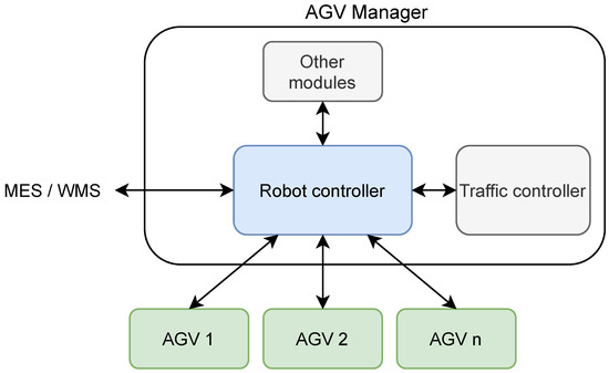
Figure 1.
General architecture of the AGV Manager.
As depicted in Figure 1, the main Robot Controller service is responsible for all AGVs’ mission and navigation control (i.e., pick-up/drop-off goods in given places, material/parts supply). To this end, the Robot Controller is able to remotely communicate with all AGVs (e.g., to send movement commands or receive feedback from onboard sensors), as well as with other equipment, such as obstacle detection devices, positioning systems or energy storage management systems. These are symbolized as Other modules in Figure 1. The Traffic controller service, which might be connected as a plugin, will compute an optimal navigation solution (set of trajectories) for the AGVs, while avoiding deadlocks and collisions. For this purpose, the current and desired positions of the AGVs, in addition to the environmental information obtained from the onboard sensors and auxiliary equipment (i.e., detection of new obstacles, blocked passages, etc.) will be supplied to the Traffic controller by the Robot Controller. Initially, a CPN model of the manufacturing plant is provided, which describes the physical layout and the possible movements actions to be performed by the AGVs in the industrial facilities. Possible places that can be held and/or occupied are also defined.
Figure 2 depicts the sequence diagram for AGV navigation in the presence of dynamic obstacles. The plant operator, a human operator (if manually operated), WMS, ERP system or MES will define the goal positions for each AGV. It has to be pointed out that the Robot Controller might offer additional services and capabilities, such as AGV energy management or material pick-up and drop-off features. After the goal positions for each AGV are defined, the trajectories to be followed by each AGV within the industrial shop floor are computed at the request of the Robot Controller. Once computed, the Robot Controller will monitor and control the navigation of each AGV through the shop floor.
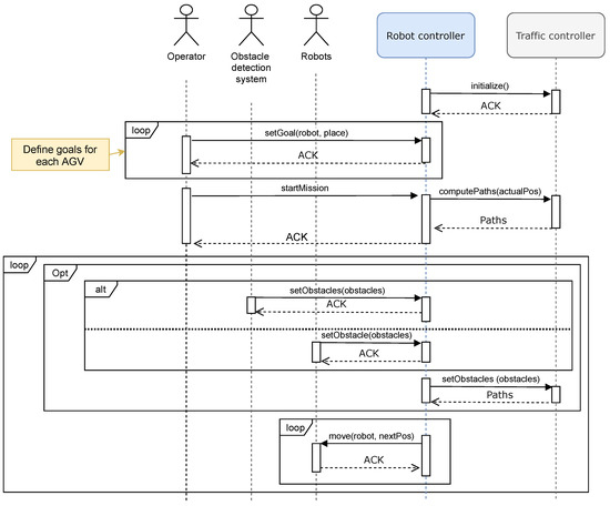
Figure 2.
AGV navigation sequence diagram.
As observed in Figure 2, in case a new obstacle is detected, both by an obstacle detection system or by onboard sensors located in the AGVs, a new set of trajectories for the AGVs might be needed. This task will be performed by the Traffic Controller for which the initial coloured Petri net model will be used as a basis for the AGVs’ trajectory replanning.
4.1. Coloured Petri Net Model
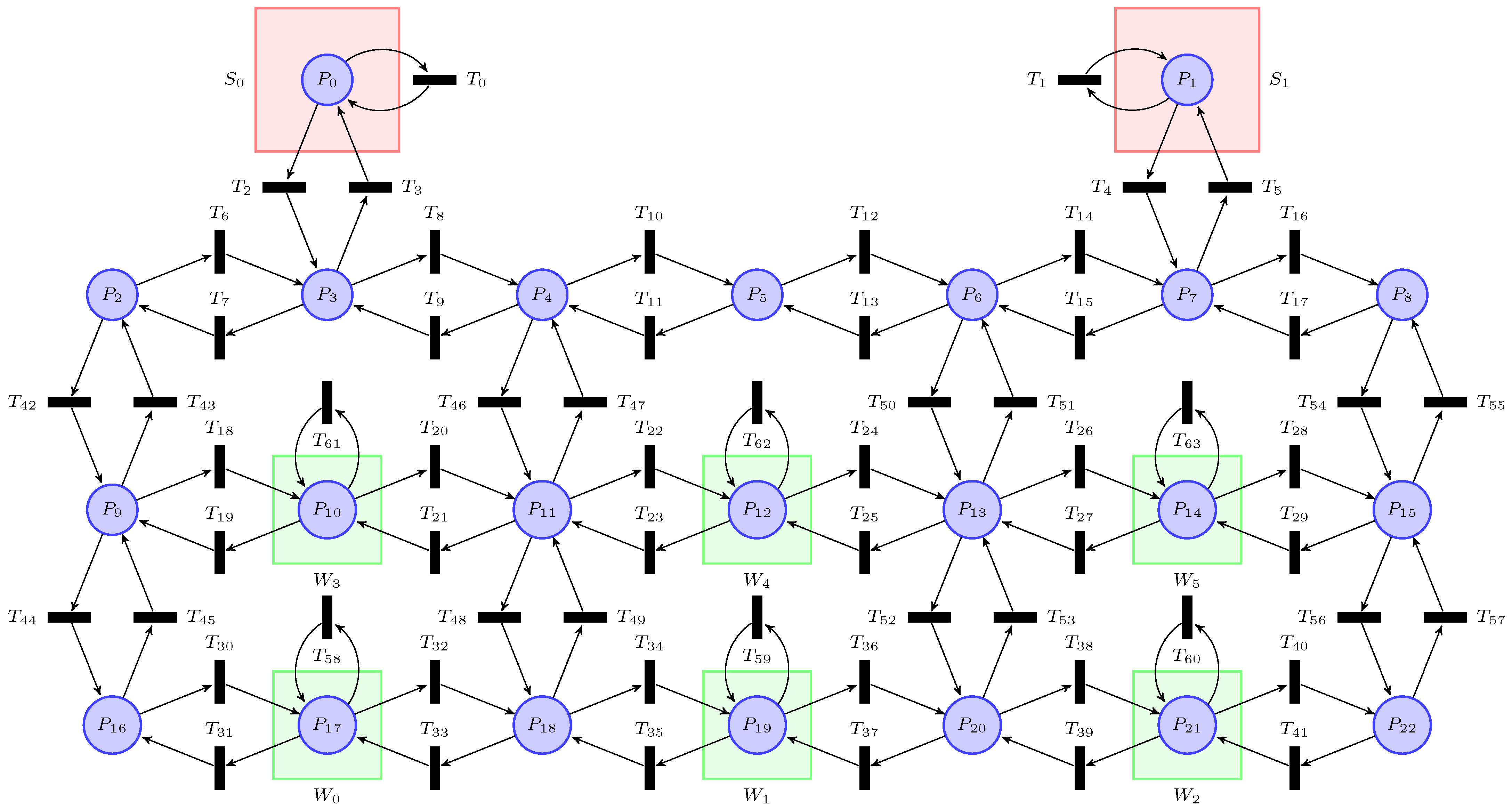
The industrial shop floor was modelled as a coloured Petri net, in which AGVs were considered tokens and different locations within the industrial shop floor places. Each AGV is defined and identified as a colour. Figure 3 depicts a CPN model of a manufacturing plant. In the model, special places are defined, which are workstations ( for in ) and storehouses ( and ).
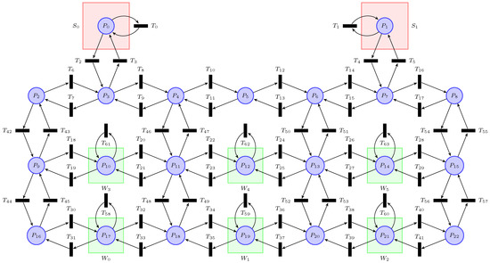
Figure 3.
Petri net model of the manufacturing facility.
The coloured Petri net model extends the classic Place/Transition (PT) net, maintaining its original features and functionalities. In particular, the assumption that a single AGV is positioned in a given place at a given time instance is made. For each place in the Petri net shown in Figure 3, different inbound and outbound transitions, for which firing enables the incoming and outgoing traffic of AGVs, are defined. Due to net colouring, in each transition, a single AGV is involved. However, in a given time instance, different transitions can be simultaneously fired, which will promote the movement of multiple AGVs.
However, particular transitions related to the modification of the attributes, the state of the AGV or the manufacturing process are defined. On the one hand, the and transitions implement storehouse functionalities, such as pick-up and drop-off functions. On the other hand, transitions to represent part/product processing functions at workstations. Through the activation of these special transitions, the state of the corresponding AGV, storehouse and/or workstation might be changed. Since these transitions are not related to the AGV traffic control and navigation, they are disabled for the AGV path planning and traffic control.
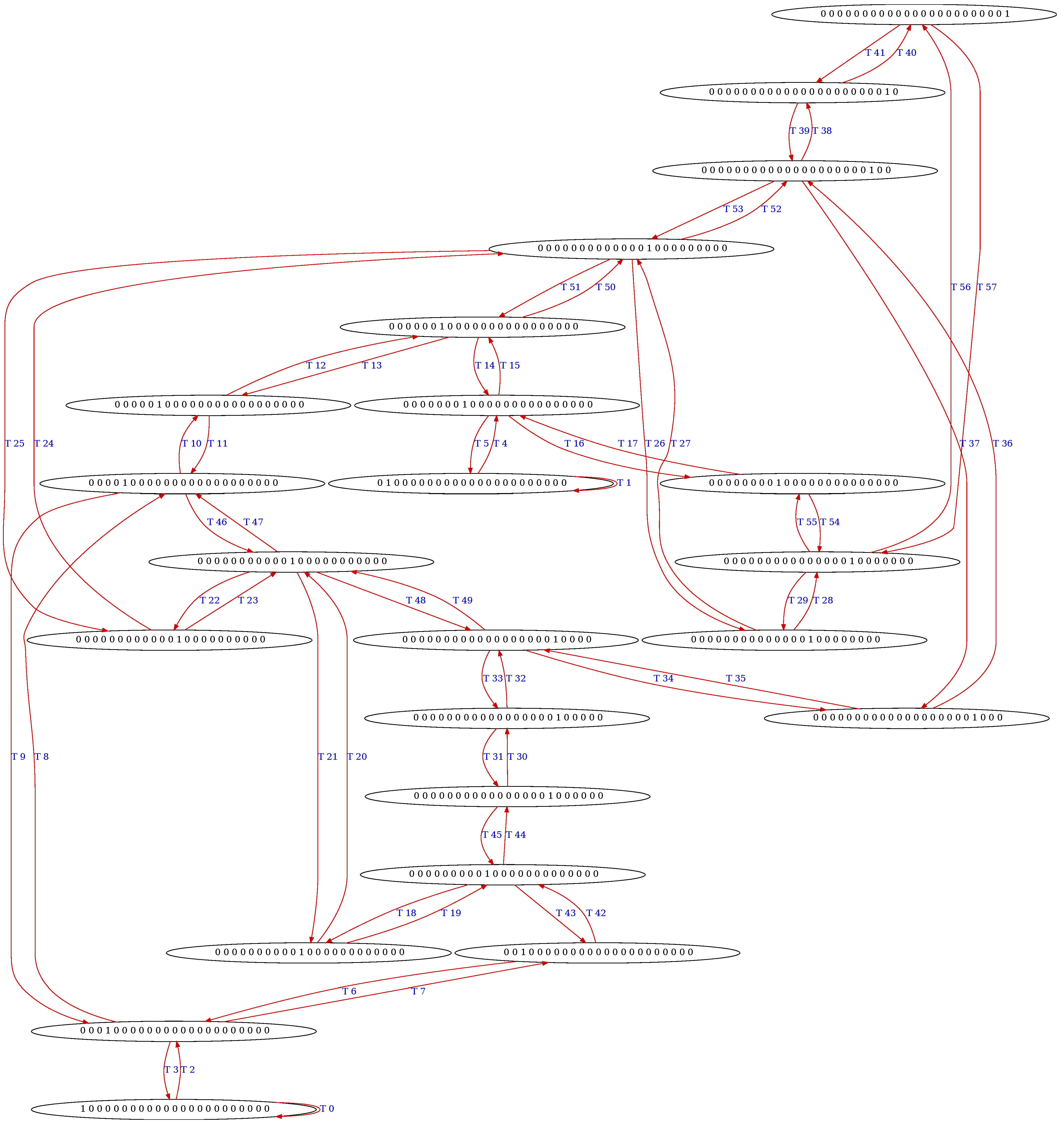
Once the CPN model is defined ( and matrices) and supplied to the Traffic Controller, the reachability graph is built. This directed graph contains all feasible AGVs position, that is the CPN markings and their progression paths. These movements are obtained using the state equation shown in Equation (1). Figure 4 shows the built reachability graph for a single AGV computed from the Petri net model shown in Figure 3, in which edges represent the transition to be activated in order to reach a new marking. On the contrary, each vertex corresponds to a CPN marking, displayed as a vector. This vector indicates where each of the AGVs is located on the shop floor; in other words, the position in the vector of the AGV identifier corresponds to the place number. A 0 implies that no AGV is positioned in such a place. When multiple AGVs are defined, those marking vector positions are filled with the corresponding AGV identifier number.
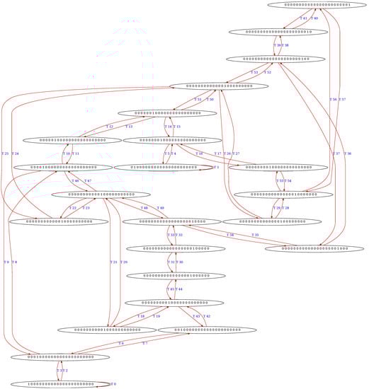
Figure 4.
Example reachability graph for a single AGV for the CPN model shown in Figure 3.
For the construction of the graph, all feasible CPN markings are initially computed. After that, for each marking, all possible successors and firings are firstly computed. To this end, a list of fireable transitions is obtained by comparing the actual marking with the incidence matrix. If is met, transition t is determined as fireable. This ensures that transitions without any token origin places are not fired. A recursion method is then employed to compute a list of possible firings. This list will contain an inventory of all possible firing vectors for a given marking. This method is shown in Algorithm 1.
| Algorithm 1 Recursive firing vector list computation. |
| emphtyFiring := () |
| list := {emphtyFiring} |
| for each fireableTransition do |
| copyList := list |
| activateTransitions(fireableTransition,copyList) |
| list.Add(copyList) |
| end for |
As depicted in Algorithm 1, a list of possible firings is initially instantiated, where an empty firing vector (no fireable transition) is inserted. Then, for each fireable and nonblocked transition, a copy of it is performed and the correspondent transition activated for all elements in the duplicated list. Lastly, all firing possibilities contained in the are appended to the original list. Moreover, the assumption that only a transition from a couple that connects two places can be activated is made, which means that only a single AGV can go through a passage each time (unidirectional road). Given the example above depicted in Figure 3, and cannot simultaneously be fired.
The recursive firing list computation shown in Algorithm 1 does not deal with this issue. As a result, the computed list is then analysed, and all firing vectors that do not fulfil this property are removed from the list. Depending on the use case, this feature of the Traffic Controller could be disabled (just omitting the last step), enabling bidirectional passages.
Following this, a list of all possible movements of AGVs, denoted successors, is obtained based on the previous state. This task is accomplished by using Equation (1). New markings are computed based on the computed firing vectors (recorded in the data structure). If any collision is detected in the new state (more than one AVG in a given place), the new possible state, and thus the coloured marking, is rejected. All descendant movements and states for each marking are calculated and, at the same time, the reachability graph built.
4.2. Trajectory Planning
For the collision-free trajectory planning and traffic control, the D* Lite searching algorithm [40] is executed throughout the initially constructed reachability graph. Unlike the usual grid-based space searching approach employed in robotics, in which each grid cell refers to a discretized physical area, this approach works at the all-at-once simultaneous multi-AGV-aware trajectory planning level. A combined solution considering multiple AGVs trajectories is computed. D* Lite, as suggested by its name, is an incremental (dynamic) heuristic searching algorithm. This algorithm, which is based on the Lifelong Planning A* (LPA*), reuses previously generated states and data to speed up the new searches, and hence save time, instead of solving the search every time from the beginning. Although it is not based on the original D* or Focused D*, it implements the same behaviour.
In order to improve the searching time, as commonly done in robotics, heuristics were used. As stated by S. Koenig and M. Likachev [40], the heuristics need to be non-negative and satisfy ( being the cost of the shortest path from vertex s to vertex ) and . An admissible heuristic should not overestimate the real cost. Therefore, the Manhattan distance was used for the heuristics, which is defined as the sum of the vertical and horizontal distances between points in a grid. The heuristic was then calculated by summing up all the Manhattan distances of all the AGVs from the actual positions of the vehicle towards the goal positions, as shown in Equation (2).
During the execution of the simulation and the D* Lite searching algorithm, the cost of edges in the reachability graph of the Petri net might change depending on if any related transition has been affected by an obstacle or not. A dynamic obstacle refers to any element (i.e., forklifts) or people that might obstruct a given zone or passage in the manufacturing plant. When a new obstacle is detected, either by a global detection system or onboard sensors (as depicted in Figure 2), this information is transmitted to the AGV Manager. The Robot Controller will specify which transitions of the CPN model became blocked. In the recomputation of the trajectories for the AGVs, the cost for the activation of those transitions, and hence the corresponding movement, was set to infinity. The D* Lite algorithm will try to come up with an alternative solution.
5. Case Study
In this section, a case study of the proposed method is presented, in which four different AGVs were considered. Furthermore, the previously depicted manufacturing shop floor model, shown in Figure 3, was used. This model is loaded into the Traffic Controller, which then constructs the reachability graph. After its initialization, the current and goal positions of the AGVs can be determined. Table 2 shows the defined initial and goal places for the AGVs.
Table 2.
Initial and goal places of the AGVs.
Once these initial and goal locations are determined, an initial trajectory is computed for each AGV by the Traffic Controller (see Figure 2). The Robot Controller would then control the navigation of the AGVs. In case an obstacle is detected, the execution of the D* Lite algorithm is triggered, from which an alternative solution to the initially calculated trajectories could be computed. The initially computed solution and the final outcome might differ. In this case study, the behaviour of the obstacle detection system and mobile robots were emulated by means of a simulation. On the one hand, the experimental results obtained through such simulation are provided. On the other hand, the performance of the Traffic Controller was evaluated in terms of expanded vertices in the D* Lite processing and employed CPU.
5.1. Experimental Results
As previously stated, after the initialization and the specification of AGV current and desired goal positions, an initial solution is computed. Figure 5 shows the initially computed solution, which shows which AGV (depicted as coloured boxes, as defined in Table 2) should be situated and/or displaced to which place at which time instance in order to reach the goal.

Figure 5.
Initially computed solution: places held by the AGVs in each time instance.
As observed in Figure 5, both and intend to go through and . On the contrary, and intend to move from to . Both and should go just behind their respective front leader. It was expected to require seven time instances, seven movements for each AGV (concurrently), to reach their goals.
During the simulation, the detection of several obstacles was emulated. In particular, three different obstacles were simulated. Table 3 shows the properties of these obstacles, specifically which passage do they obstruct, which transitions are blocked and at which time instances are enabled and disabled in the simulation.
Table 3.
Emulated dynamic obstacles.
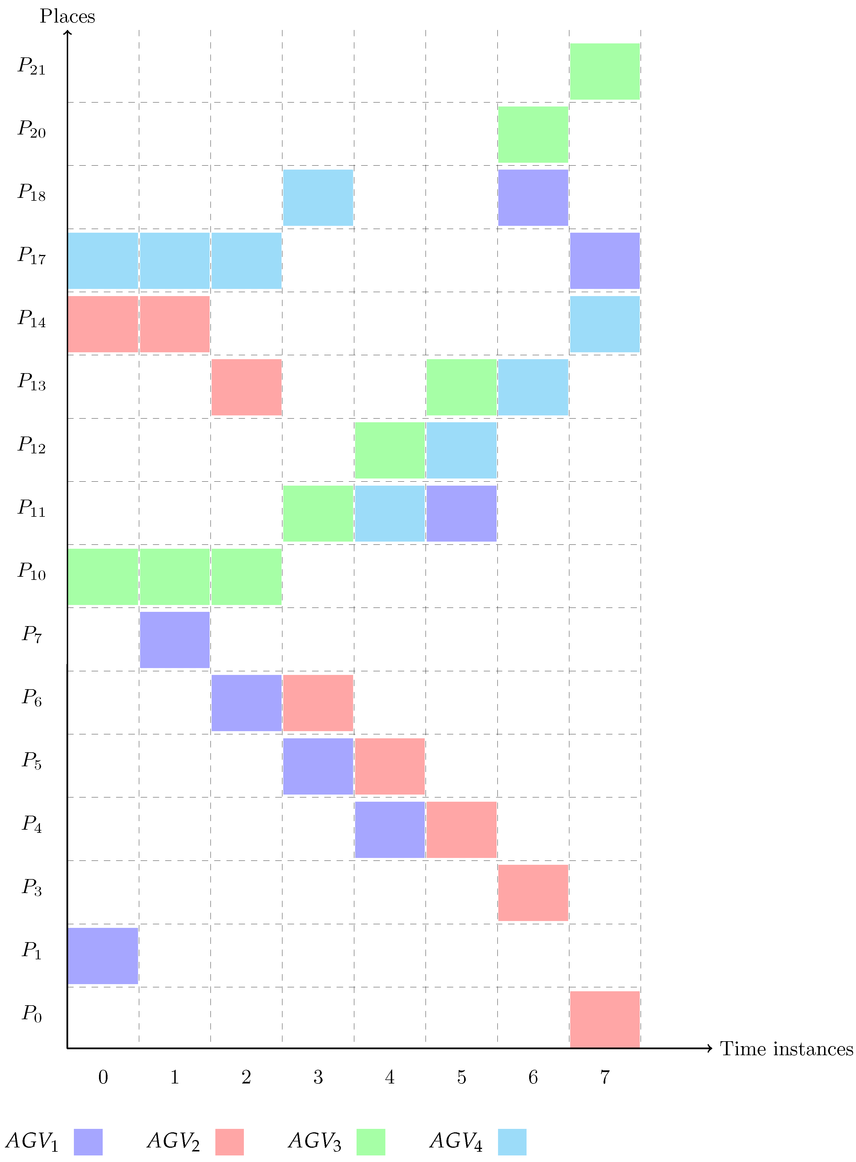
Figure 6 shows the AGV trajectories obtained in the simulation, in which the dynamic obstacles shown in Table 3 were considered and avoided (similarly to Figure 5, and AGVs are shown as coloured boxes as defined in Table 2). As can be observed, different trajectories to the ones computed initially (shown in Figure 5) were followed by the AGVs in order to avoid the obstacles. The AGVs required, as a whole, two more steps to reach their goal positions. Due to obstacle , the passage between and (initially considered and planned at Time Instances 4 and 5) was avoided by and . Both robots drove across the downside track of the manufacturing shop floor to reach the goal, instead of using the middle track, as initially estimated.
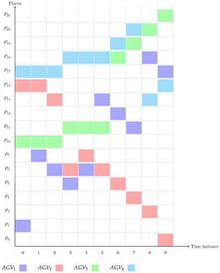
Figure 6.
Simulation output: places held by the AGVs in each time instance.
Moreover, since the road between and was later in the blocked state (at Time Instance 4 by ), required stepping backwards to and moving through the route between and . The passage through and (free after Time Instance 4) was then used by . It is worth pointing out that obstacle did not affect the outcome of the simulation.
Both in the initially computed solution and in the simulation output, and needed to wait some time in a given position. Meanwhile, and took advantage of the situation and exchanged their positions in the upper and middle tracks of the manufacturing shop floor. This behaviour, addressed by the D* Lite algorithm, avoided any future deadlocks.
5.2. Performance Evaluation
In this subsection, the performance of the proposed approach is evaluated. For this purpose, the number of evaluated vertices in the computation of the solution by the D* Lite algorithm was obtained and the employed CPU time measured. Figure 7 shows the number of evaluated vertices from the reachability graph throughout the simulation. The Traffic Controller required a low number of evaluations at Time Instances 2 and 6 for the AGV trajectories replanning. However, at Time Instance 4, the system came to the conclusion that should move backwards, since passages and were not available. Five more evaluations comparing to the computation of the initial solution were then needed in order to overcome the obstacle.
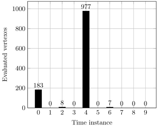
Figure 7.
Evaluated vertices from the reachability graph throughout the simulation.
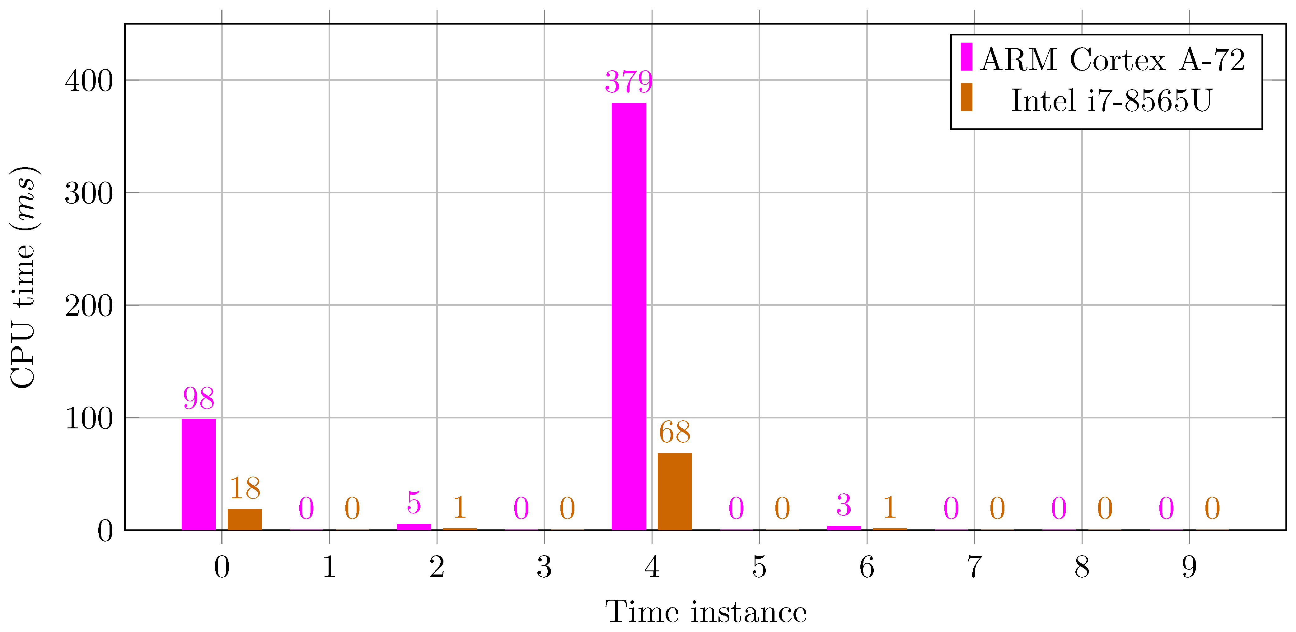
As far as the required processing capabilities are concerned, the utilized CPU time was measured. The Traffic Controller service was executed on two different hardware platforms, an ARM-based embedded board (ARM Cortex-A72 (ARM Inc., Cambridge, UK) running at 1.5 GHz) and on an x86 personal computer (Intel i7-8565U (Intel Inc., Santa Clara, CA, USA) CPU running up to 4.60 GHz). Figure 8 shows the employed CPU time for the computation of the AGV trajectories throughout the simulation in both hardware platforms. It has to be noted that these measurements may vary depending on the selected programming language and/or employed technology. The Traffic Controller service was implemented in Ada. This programming language is widely used in the safety domain [39], as well as for the development of air traffic management systems [41].

Figure 8.
Employed CPU time for the computation of the AGV trajectories.
As depicted in Figure 8, for the computation of the initial solution, the Traffic Controller required 98 ms (ARM Cortex A-72) and 18 ms (Intel I7-8565U), respectively. At Time Instance 4, where higher processing for the recalculation of trajectories was needed, 379 ms and 68 ms of CPU time were employed. Otherwise, since the searching algorithm tried to reuse previously generated information, low processing overhead was evaluated at Time Instances 2 and 6. In both cases, less than a millisecond of CPU time was measured on the personal computer. As noted, the computational capabilities of the selected hardware platform play an important role.
6. Discussion
In contrast to the methods and techniques discussed in the Related Work Section, the method proposed in this article provides a formally verifiable dynamic traffic management system. The main advantage over other suggested techniques is the avoidance of deadlocks; this is because, instead of managing each AGV independently or locally, the traffic controller considers all the moves of all AGVs. As shown in the presented case study, in which the traffic management and navigation of four AGVs were handled, the proposed approach provides a formally verifiable, sound and robust AGV path planning and traffic controlling method. Furthermore, according to the obtained experimental results, the implemented Traffic Controller, executed in two different hardware platforms, showed good real-time performance, requiring, in the worst case, less than half a second of processing time.
As observed, the computation performance is considerably improved if high-performance computing systems are used. Nevertheless, an important drawback of the proposed approach is the exponential increase of the reachability graph size as the shop floor area and the number of AGVs grow. The size of the graph depended on the CPN model (defined places and transitions) and the amount of considered AGVs. In order to overcome this constraint, dynamic graph data structures might be used. However, this technique will, most probably, introduce computation overheads. The presented method could be applied, for example, in the fabric manufacturing enterprise case study presented by Okumuş et al. [1].
7. Conclusions and Future Work
In the scope of the Industry 4.0 revolution, advanced digital and computer-based technologies (e.g., big data, IIoT) are incorporated for increased self-monitoring, automation and production. In these smart factories, higher cooperation among cyber-physical systems, such as AGVs, and humans is envisioned. By means of the provided advanced connectivity and processing features, these intelligent systems may enable dynamic and cost-effective internal flows of goods with minimal human input. However, since AGVs might share industrial areas and routes with operators, a trustworthy and efficient collision avoidance mechanism should be enforced. This topic was tackled in the European Plug And Navigate (PAN)-Robots project [17,18,19]. In addition to an advanced sensing system, macroscopic-level fleet and traffic management features were examined.
In this article, a CPN- and D* Lite-based [40] traffic controller was proposed, which dynamically determines collision-free trajectories for the AGVs. Due to the employed formal method technique, possible deadlocks were also prevented. To this end, the reachability graph was firstly computed. For the computation of paths, the well-known D* Lite algorithm [40] was executed throughout the created reachability graph. D* Lite, which is an incremental (dynamic) searching algorithm, reuses previously generated states and data to speed up new searches, instead of computing the solution every time from the start.
For future work, the real-time performance of the traffic controller on real industrial manufacturing and/or warehouse facilities could be evaluated. In this analysis, different amounts of AGVs should be considered and timing variations measured. A systematic study, for example by means of benchmarking, may also be performed to evaluate and characterize the applicability and boundary of the proposed approach for large-scale CPN models. This evaluation should also consider and assess different computation platforms. Moreover, as previously stated, the use of dynamic graph data structures should also be investigated.
Author Contributions
Conceptualization, I.M. and J.C.M.; Formal analysis, J.C.M.; Investigation, I.M.; Software, I.M.; Writing—original draft, J.C.M.; Writing—review and editing, I.M. and J.C.M. All authors have read and agreed to the published version of the manuscript.
Funding
This research received no external funding.
Data Availability Statement
Data available on request due to restrictions eg privacy or ethical.
Conflicts of Interest
The authors declare no conflict of interest.
References
- Okumuş, F.; Dönmez, E.; Kocamaz, A.F. A cloudware architecture for collaboration of multiple agvs in indoor logistics: Case study in fabric manufacturing enterprises. Electronics 2020, 9, 2023. [Google Scholar] [CrossRef]
- Mugarza, I.; Mugarza, J.C. Towards Collision-Free Automated Guided Vehicles Navigation and Traffic Control. In Proceedings of the 2019 24th IEEE International Conference on Emerging Technologies and Factory Automation (ETFA), Zaragoza, Spain, 1–10 September 2019; pp. 1599–1602. [Google Scholar]
- Petri, C.A. Kommunikation Mit Automaten. Ph.D. Thesis, University of Hamburg, Hamburg, Germany, 1962. [Google Scholar]
- Holloway, L.E.; Krogh, B.H.; Giua, A. A survey of Petri net methods for controlled discrete event systems. Discret. Event Dyn. Syst. 1997, 7, 151–190. [Google Scholar] [CrossRef]
- Murata, T. Petri nets: Properties, analysis and applications. Proc. IEEE 1989, 77, 541–580. [Google Scholar] [CrossRef]
- Peterson, J.L. Petri Net Theory and the Modeling of Systems; Prentice Hall: Hoboken, NJ, USA, 1981. [Google Scholar]
- Reisig, W.; Rozenberg, G. Lectures on Petri Nets I: Basic Models: Advances in Petri Nets; Springer Science & Business Media: Berlin/Heidelberg, Germany, 1998. [Google Scholar]
- Talebberrouane, M.; Khan, F.; Lounis, Z. Availability analysis of safety critical systems using advanced fault tree and stochastic Petri net formalisms. J. Loss Prev. Process Ind. 2016, 44, 193–203. [Google Scholar] [CrossRef]
- Leveson, N.G.; Stolzy, J.L. Safety analysis using Petri nets. IEEE Trans. Softw. Eng. 1987, 3, 386–397. [Google Scholar] [CrossRef]
- Adamyan, A.; He, D. Failure and safety assessment of systems using Petri nets. In Proceedings of the 2002 IEEE International Conference on Robotics and Automation (Cat. No. 02CH37292), Washington, DC, USA, 11–15 May 2002; Volume 2, pp. 1919–1924. [Google Scholar]
- Jensen, K. Coloured Petri nets and the invariant-method. Theor. Comput. Sci. 1981, 14, 317–336. [Google Scholar] [CrossRef] [Green Version]
- Jensen, K. Coloured petri nets. In Petri Nets: Central Models and Their Properties; Springer: Berlin/Heidelberg, Germany, 1987; pp. 248–299. [Google Scholar]
- Jensen, K. Coloured Petri Nets: Basic Concepts, Analysis Methods and Practical Use; Springer Science & Business Media: Berlin/Heidelberg, Germany, 2013; Volume 1. [Google Scholar]
- Raineri, M.; Perri, S.; Bianco, C.G.L. Online velocity planner for Laser Guided Vehicles subject to safety constraints. In Proceedings of the 2017 IEEE/RSJ International Conference on Intelligent Robots and Systems (IROS), Vancouver, BC, Canada, 24–28 September 2017; pp. 6178–6184. [Google Scholar]
- Raineri, M.; Perri, S.; Bianco, C.G.L. Safety and efficiency management in LGV operated warehouses. Robot. Comput.-Integr. Manuf. 2019, 57, 73–85. [Google Scholar] [CrossRef]
- Fazlollahtabar, H.; Saidi-Mehrabad, M.; Balakrishnan, J. Mathematical optimization for earliness/tardiness minimization in a multiple automated guided vehicle manufacturing system via integrated heuristic algorithms. Robot. Auton. Syst. 2015, 72, 131–138. [Google Scholar] [CrossRef]
- Sabattini, L.; Aikio, M.; Beinschob, P.; Boehning, M.; Cardarelli, E.; Digani, V.; Krengel, A.; Magnani, M.; Mandici, S.; Oleari, F.; et al. The pan-robots project: Advanced automated guided vehicle systems for industrial logistics. IEEE Robot. Autom. Mag. 2017, 25, 55–64. [Google Scholar] [CrossRef]
- Cardarelli, E.; Sabattini, L.; Digani, V.; Secchi, C.; Fantuzzi, C. Interacting with a multi AGV system. In Proceedings of the 2015 IEEE International Conference on Intelligent Computer Communication and Processing (ICCP), Cluj-Napoca, Romania, 3–5 September 2015; pp. 263–267. [Google Scholar]
- Sabattini, L.; Cardarelli, E.; Digani, V.; Secchi, C.; Fantuzzi, C.; Fuerstenberg, K. Advanced sensing and control techniques for multi AGV systems in shared industrial environments. In Proceedings of the 2015 IEEE 20th Conference on Emerging Technologies & Factory Automation (ETFA), Luxembourg, 8–11 September 2015; pp. 1–7. [Google Scholar]
- Stentz, A. Optimal and efficient path planning for partially known environments. In Intelligent Unmanned Ground Vehicles; Springer: Berlin/Heidelberg, Germany, 1997; pp. 203–220. [Google Scholar]
- Zhang, Z.; Guo, Q.; Chen, J.; Yuan, P. Collision-Free Route Planning for Multiple AGVs in an Automated Warehouse Based on Collision Classification. IEEE Access 2018, 6, 26022–26035. [Google Scholar] [CrossRef]
- Silver, D. Cooperative Pathfinding. AIIDE 2005, 1, 117–122. [Google Scholar]
- Wang, C.; Wang, L.; Qin, J.; Wu, Z.; Duan, L.; Li, Z.; Cao, M.; Ou, X.; Su, X.; Li, W.; et al. Path planning of automated guided vehicles based on improved A-Star algorithm. In Proceedings of the 2015 IEEE International Conference on Information and Automation, Lijiang, China, 8–10 August 2015; pp. 2071–2076. [Google Scholar]
- Xiao, H.; Wu, X.; Zeng, Y.; Zhai, J. A CEGA-Based Optimization Approach for Integrated Designing of a Unidirectional Guide-Path Network and Scheduling of AGVs. Math. Probl. Eng. 2020, 2020, 1–16. [Google Scholar] [CrossRef] [Green Version]
- Zou, W.Q.; Pan, Q.K.; Tasgetiren, M.F. An effective discrete artificial bee colony algorithm for scheduling an Automatic-Guided-Vehicle in a linear manufacturing workshop. IEEE Access 2020, 8, 35063–35076. [Google Scholar] [CrossRef]
- Li, B.; Liu, H.; Xiao, D.; Yu, G.; Zhang, Y. Centralized and optimal motion planning for large-scale AGV systems: A generic approach. Adv. Eng. Softw. 2017, 106, 33–46. [Google Scholar] [CrossRef]
- Lyu, X.; Song, Y.; He, C.; Lei, Q.; Guo, W. Approach to integrated scheduling problems considering optimal number of automated guided vehicles and conflict-free routing in flexible manufacturing systems. IEEE Access 2019, 7, 74909–74924. [Google Scholar] [CrossRef]
- Draganjac, I.; Petrović, T.; Miklić, D.; Kovačić, Z.; Oršulić, J. Highly-scalable traffic management of autonomous industrial transportation systems. Robot. Comput.-Integr. Manuf. 2020, 63, 101915. [Google Scholar] [CrossRef]
- Maw, A.A.; Tyan, M.; Nguyen, T.A.; Lee, J.W. iADA*-RL: Anytime Graph-Based Path Planning with Deep Reinforcement Learning for an Autonomous UAV. Appl. Sci. 2021, 11, 3948. [Google Scholar] [CrossRef]
- Herrero-Perez, D.; Martinez-Barbera, H. Modeling distributed transportation systems composed of flexible automated guided vehicles in flexible manufacturing systems. IEEE Trans. Ind. Inform. 2010, 6, 166–180. [Google Scholar] [CrossRef]
- Wu, N.; Zhou, M. Shortest routing of bidirectional automated guided vehicles avoiding deadlock and blocking. IEEE/ASME Trans. Mechatron. 2007, 12, 63–72. [Google Scholar] [CrossRef]
- Fazlollahtabar, H.; Saidi-Mehrabad, M. Methodologies to optimize automated guided vehicle scheduling and routing problems: A review study. J. Intell. Robot. Syst. 2015, 77, 525–545. [Google Scholar] [CrossRef]
- Aized, T. Modelling and performance maximization of an integrated automated guided vehicle system using coloured Petri net and response surface methods. Comput. Ind. Eng. 2009, 57, 822–831. [Google Scholar] [CrossRef]
- Baruwa, O.T.; Piera, M.A. A coloured Petri net-based hybrid heuristic search approach to simultaneous scheduling of machines and automated guided vehicles. Int. J. Prod. Res. 2016, 54, 4773–4792. [Google Scholar] [CrossRef]
- Baruwa, O.T.; Piera, M.A.; Guasch, A. TIMSPAT–Reachability graph search-based optimization tool for colored Petri net-based scheduling. Comput. Ind. Eng. 2016, 101, 372–390. [Google Scholar] [CrossRef] [Green Version]
- Giua, A.; Seatzu, C. Modeling and supervisory control of railway networks using Petri nets. IEEE Trans. Autom. Sci. Eng. 2008, 5, 431–445. [Google Scholar] [CrossRef]
- Giglio, D.; Sacco, N. A Petri net model for analysis, optimisation, and control of railway networks and train schedules. In Proceedings of the 2016 IEEE 19th International Conference on Intelligent Transportation Systems (ITSC), Rio de Janeiro, Brazil, 1–4 November 2016; pp. 2442–2449. [Google Scholar]
- Sun, P. Model Based System Engineering for Safety of Railway Critical Systems. Ph.D. Thesis, Ecole Centrale de Lille, Villeneuve-d’Ascq, France, 2015. [Google Scholar]
- International Electrotechnical Commission. IEC 61508: Functional Safety of Electrical/Electronic/Programmable Electronic Safety-Related Systems; International Electrotechnical Commission: London, UK, 2010. [Google Scholar]
- Koenig, S.; Likhachev, M. Dˆ* Lite. Aaai/Iaai 2002, 15. [Google Scholar]
- Srivastava, A.; Woodard, F.; O’Leary, J. Ada’s Vital Role in New US Air Traffic Control Systems. In Proceedings of the International MultiConference of Engineers and Computer Scientists. Citeseer, Hong Kong, China, 18–20 March 2009; Volume 1. [Google Scholar]


Publisher’s Note: MDPI stays neutral with regard to jurisdictional claims in published maps and institutional affiliations. |
© 2021 by the authors. Licensee MDPI, Basel, Switzerland. This article is an open access article distributed under the terms and conditions of the Creative Commons Attribution (CC BY) license (https://creativecommons.org/licenses/by/4.0/).