Abstract
In recent years, artificial intelligence technology has been widely used in fault prediction and health management (PHM). The machine learning algorithm is widely used in the condition monitoring of rotating machines, and normal and fault data can be obtained through the data acquisition and monitoring system. After analyzing the data and establishing a model, the system can automatically learn the features from the input data to predict the failure of the maintenance and diagnosis equipment, which is important for motor maintenance. This research proposes a medium Gaussian support vector machine (SVM) method for the application of machine learning and constructs a feature space by extracting the characteristics of the vibration signal collected on the spot based on experience. Different methods were used to cluster and classify features to classify motor health. The influence of different Gaussian kernel functions, such as fine, medium, and coarse, on the performance of the SVM algorithm was analyzed. The experimental data verify the performance of various models through the data set released by the Case Western Reserve University Motor Bearing Data Center. As the motor often has noise interference in the actual application environment, a simulated Gaussian white noise was added to the original vibration data in order to verify the performance of the research method in a noisy environment. The results summarize the classification results of related motor data sets derived recently from the use of motor fault detection and diagnosis using different machine learning algorithms. The results show that the medium Gaussian SVM method improves the reliability and accuracy of motor bearing fault estimation, detection, and identification under variable crack-size and load conditions. This paper also provides a detailed discussion of the predictive analytical capabilities of machine learning algorithms, which can be used as a reference for the future motor predictive maintenance analysis of electric vehicles.
1. Introduction
Mechanical fault diagnosis technology involves the monitoring, diagnosis, and early warning of the status and faults of continuously operating mechanical equipment. In other words, it is a science and technology to ensure the safe operation of machinery and equipment. It is a new discipline that has developed rapidly in recent years with the help of modern technological achievements in multiple disciplines. Rolling bearings are one of the important components of rotating machinery and equipment. The quality of its running state is directly related to the running state of the rotating equipment. Therefore, the research on real-time monitoring and fault diagnosis of the working conditions of rolling bearings has received increasing attention from researchers. The current research literature and current situation are explained in the subsequent section.
1.1. Theoretical Research in Data Acquisition and Sensing Technology
Reliable signal acquisition and advanced sensing technology are the prerequisites for mechanical fault diagnosis. A sensor is a detection device that can feel the information being measured and can sense the information. It transforms into electrical signals or other required forms of information output according to certain rules to meet the requirements of information transmission, processing, storage, display, recording, and control. It is usually divided into vibration sensor, temperature sensor, light sensor, gas sensor, pressure sensor, magnetic sensor, humidity sensor, sound sensor, radiation sensor, color sensor, etc. Temperature monitoring method, when the equipment is running abnormally, the temperature of its parts will also change. By monitoring the temperature change, the defects and damages of the mechanical equipment can be found. The sound sensor is to receive the impact signal generated by the impact and friction of metal materials and the fracture of metal parts. The early surface of the bearing is slightly damaged, from plastic deformation to fracture failure of the bearing component. When the bearing encounters these defects during the working process, a transient elastic stress wave will be generated, and energy will be released. Vibration sensors measure the dynamic characteristics of mechanical equipment, which can be expressed through vibration signals. By analyzing and processing the rich information, the working status and faults of the equipment can be obtained. Johnson [1] studied a model of sequential diagnostic test procedures to be applied to fault location in electronic equipment. Preparata et al. [2] developed the automatic fault diagnosis problem of multi-fault systems on the connection allocation problem of the diagnosable system. Sohre [3,4] summarized the vibration characteristic analysis table based on the analysis experience of more than 600 accidents. Based on this, Jackson [5] compiled the general change rule table of the vibration analysis characteristics of rotating machinery, which was widely cited by researchers in the condition monitoring and fault diagnosis analysis of rotating machinery. Professor Achenbach [6] led an important discussion of structural health monitoring research and listed sensor technology as an important research topic. Nair [7] researched sensor networks, and Park et al. [8] researched sensor layout. Takeda et al. [9] conducted significant research on the health monitoring and sensing of the and composite material structure. There are many related studies in this field [10,11,12].
1.2. Fault Mechanism and Symptom Relationship
Understanding the mechanism and characterization of faults is the basis of mechanical fault diagnosis. Common mechanical failure modes are as follows: (1) failure in the material performance of mechanical parts, including fatigue, fracture, crack, creep, excessive deformation, material deterioration, etc.; (2) faults that belong to abnormal chemical and physical conditions, including corrosion, grease degradation, insulation degradation, electrical and thermal conductivity degradation, evaporation, etc.; (3) fault in the motion state of mechanical equipment, including vibration, leakage, blockage, abnormal noise, etc.; (4) failure in the comprehensive performance due to multiple reasons, such as wear, overplaying or loss of interference of mating parts, loosening and failure of fixing and fastening devices, etc. Italian scholars Bachschmid and Pennacchi [13] commemorated the 50th anniversary of crack research, edited a review article on crack research in the international journal MSSP, and led relevant discussions of the cracked rotor model and crack mechanism. Gasch et al. [14] studied the dynamic behavior of cracked rotors. Chen et al. [15] conducted extensive research on practical technologies, such as fault mechanism and feature extraction. Sekhar [16] studied the dynamic behavior of rotor cracks and their identification methods. Peng et al. [17] made significant progress in the theoretical research of wavelet transform and the mechanism of rotor rubbing faults. Immovilli et al. [18] studied the spectral kurtosis energy of vibration or current signals to detect generalized-roughness bearing faults. The method was verified by experiments on vibration signals, and the results were robust and reliable. Immovilli et al. [19] compared the bearing fault detection capabilities obtained by studying vibration and current signals. There are many related studies in this field [20,21,22].
1.3. Data Analysis and Diagnosis Method
It is necessary to extract fault signs from the running dynamic signals for mechanical fault diagnosis. Jardine et al. [23], who have been engaged in maintenance and reliability research in Canada for a long time, pointed out that methods, such as signal processing and fault diagnosis, need to be further studied. Mehrjou et al. [24] summarized various common rotor fault types, discussed the principles and characteristics of various state monitoring and signal processing methods, and summarized the results of research on current rotor fault diagnosis. Gebraeel et al. [25] suggested new ideas for research on machine tool manufacturing and life prediction. Ihn et al. [26] reported significant results in research on the health monitoring of composite structures. Gao and Yan [27,28] published a wavelet analysis book on fault diagnosis. Gu et al. [29] have been engaged in fault diagnosis research for a long time. Zhen et al. [30] studied the improved cyclic modulation spectrum analysis of the CWT method and its application in the fault diagnosis of induction motor rotor broken bars. There are many related studies in this field [31,32,33].
1.4. Intelligent Decision and Diagnosis System
Intelligent fault diagnosis is a reasoning process that simulates human thinking through effective acquisition, transmission, and processing of diagnostic information. It can simulate human experts and make intelligent judgments and decisions on the running status and faults of the monitored objects with flexible diagnosis strategies. Intelligent fault diagnosis has a learning function and the ability to automatically obtain diagnostic information for real-time fault diagnosis. Intelligent diagnosis technology and a practical diagnosis system of complex mechanical equipment faults are key to realizing the application of mechanical fault diagnosis. Professor Kruzic [34] wrote an article “Predicting Fatigue Failures” in Science, which emphasized the importance of structural fatigue life prediction research. Heng [35] reviewed the progress in research on fault diagnosis technology for rotating machinery and emphasized the importance of conducting fault diagnosis research in combination with real working conditions. Piltan et al. [36] studied the use of machine learning in rolling bearing fault diagnosis, a new technology based on an advanced fuzzy sliding mode observer. Chen et al. [37] studied the electrical, mechanical, and magnetic fault diagnosis of permanent magnet synchronous motors. They listed common faults, model-based fault diagnosis, different signal processing methods, data-driven diagnosis algorithms, and other intelligent diagnosis algorithms. Dineva et al. [38] pointed out that the presence of interference noise or multiple faults causes feature overlap. They proposed a multi-label classification method for simultaneously diagnosing multiple faults and assessing the severity of faults under noisy conditions. Li et al. [39] proposed a fault diagnosis method that combines wavelet packet transform (WPT) and a convolutional neural network (CNN). Research conclusions show that this method has fault diagnosis capabilities superior to those of other machine-learning-based methods. You [40] studied the use of a multi-layer perceptron (MLP) deep learning model to optimize the shape of the permanent magnet synchronous motor (PMSM) of an electric vehicle (EV) and redesigned the PMSM to improve the failure factor. Zhou and Tang [41] proposed a two-level Gaussian process and Bayesian inference, based on multiple levels of corresponding available data to improve the quality of a specific output data set to improve response change prediction. Li et al. [42] proposed a new data-driven method based on Gaussian process classifiers (GPCs) to classify and predict turbine failures. Zhou and Tang [43] proposed the use of adaptive multi-response Gaussian process meta-modeling and established an adaptive sampling strategy to guide the search of unknown parameters. The research proved the high efficiency and accuracy of the new framework. Mansouri et al. [44] proposed a new application of Interval Gaussian process regression (IGPR)-based random forest (RF) technology (IGPR-RF) in wind energy conversion systems to improve the accuracy of fault classification. Wang et al. [45] proposed a new cross-domain feature-learning–transfer-learning method named probabilistic transfer factor analysis (PTFA) and applied it to gearbox fault diagnosis. Wang et al. [46] proposed an integrated fault diagnosis and prediction framework based on wavelet transform and prediction through Bayesian inference. The research is used to predict wind turbine bearing defects with limited data measurement, and its effectiveness is verified by a set of limited samples. Zhou and Tang [47] researched and established a new fuzzy classification method to deal with gear fault diagnosis with limited data labels. The accuracy rate in these two cases successfully classifies the invisible data as close to the adjacent fault category.
Mechanical fault diagnosis is essentially a problem of pattern recognition. At present, the most widely used pattern recognition methods are cluster analysis, artificial neural network (ANN), and SVM. The cluster analysis method lacks versatility and has a large amount of calculation. ANN method has strong self-organization, self-learning ability, and nonlinear pattern classification ability, but it needs a large number of typical fault samples, and in the engineering practice of mechanical fault diagnosis, typical fault samples are often lacking. At the same time, the neural network has the limitations of learning, the choice of structure and type is too dependent on prior knowledge, and these limitations will seriously affect the recognition accuracy.
Based on the above literature (Section 1.1, Section 1.2, Section 1.3 and Section 1.4), these studies have their own characteristics and contributions. In recent years, smart machinery has integrated industry 4.0 technical elements to enable it to have intelligent functions such as failure prediction, accuracy compensation, automatic parameter setting, and automatic scheduling. Machine learning algorithms are often used to monitor the health of rotating machinery, by using various sensors to sense the operating status of the key modules of the equipment and trying to find out the early signs of failure before the equipment fails. In addition to finding out the early signs of failure, it also facilitates preventive maintenance early to reduce the huge losses caused by the unexpected failure of the equipment. Maintenance costs have a decisive impact. SVM is a type of machine learning algorithm that has received widespread attention in recent years. It is based on statistical learning theory and is a powerful tool in supervised classification technology.
SVM has the following main characteristics:
(1) Nonlinear mapping is the theoretical basis of the SVM method. SVM uses the inner product kernel function to replace nonlinear mapping with high-dimensional space. It is assumed that the data are linearly separable, that is, there is a separable hyperplane that can separate the two types of data, but most of them are not linearly separable in reality. The SVM kernel function can classify nonlinear data sets such as image classification, image recognition, and speech recognition;
(2) The optimal hyperplane to divide the feature space is the goal of SVM, and the idea of maximizing the classification margin is the core of the SVM method. SVM needs training data (with known data features and labels) to build the best model, and it predicts the label under known features during testing;
(3) Support vector is the training result of SVM, and it is the support vector that plays a decisive role in SVM classification decision. Applications such as stock rise or fall, credit card fraud (abnormal) prediction, and customer products are recommended;
(4) SVM is a novel small sample learning method with a solid theoretical foundation. In some practical situations, large sample data, such as rare medical disease data, cannot be obtained;
(5) The final decision function of SVM is determined by only a few support vectors, and the complexity of calculation depends on the number of support vectors, not the dimensionality of the sample space. This avoids the “curse of dimensionality” in a sense. The introduction of the kernel function avoids the “curse of dimensionality” and greatly reduces the amount of calculation. The curse of dimensionality is that in order to obtain a better classification effect, some cases need to add more features. With the increase in the number of features, although the result of the classifier fitting is more accurate, the density of the data in the space will decrease sharply. Therefore, SVM maps low-dimensional data to high-dimensional data so that nonlinearly separable data under low dimensionality are mapped to high-dimensional data and then become linearly separable. Therefore, the introduction of too many dimensions can be avoided, and there will be no dimensionality disaster. It is used in cases that require many features, such as medical gene classification or prediction.
SVM has the following main disadvantages:
(1) If the feature dimension is much larger than the number of data, the SVM performance is average;
(2) SVM is not suitable for use when the sample size is very large, and the kernel function mapping dimension is very high; hence, the calculation amount is too large;
(3) There is no universal standard for the choice of kernel function for nonlinear problems, and it is difficult to choose a suitable kernel function;
(4) SVM is sensitive to missing data.
One of the most important design choices for SVM is the kernel function. Savas and Dovisu [48] developed the application of the Gaussian kernel of SVM in a global navigation satellite system. The study applied fine, medium, and coarse Gaussian kernel function SVM classifiers. This result shows that the performance of different kernels (medium, coarse, or fine Gaussian kernels) varies depending on the data to be analyzed, resulting in differences in accuracy results. As the performance of SVM is greatly affected by the choice of kernel. It implicitly defines the structure of the high-dimensional feature space, in which the maximum edge hyperplane will be found. Commonly used kernel functions include polynomial kernel function, Gaussian kernel function, Sigmoid kernel function, and radial basis function. However, because of the different cases, the selection of kernel function pairs is also different, because different kernels may show different performances.
This research proposes three Gaussian and kernel function SVM methods in the application of machine learning and constructs a feature space by extracting the features of vibration signals collected on the spot based on experience. These methods are used to cluster and classify feature values to achieve the classification of motor health. In this study, the influence of different Gaussian kernel functions such as fine, medium, and coarse on the performance of the support vector machine algorithm was analyzed. The experimental data verified the performance of various models through the data set released by Case Western Reserve University Motor Bearing Data Center. Compared with fine and coarse Gaussian SVMs in the fault diagnosis experiment, this study proposed a medium Gaussian SVM. The average diagnosis accuracy of this method is 96%, which is 6.4% and 2.4% higher, respectively, than the other two SVMs. The medium Gaussian SVM model provides accurate cross-domain fault diagnosis. In addition, in fault diagnosis, the accuracy of the prediction of the nine features of the motor bearing when only one feature is used is 73%. Another contribution of this research is a detailed analysis and characterization of the bearing failure data of electric motors. Therefore, this study explored the results and analysis of several machine learning algorithms and their application in future motor predictive maintenance analysis.
2. Research Methodology
Machine learning involves the classification of chaotic data collected through algorithms. Several methods of machine learning are described in [49]. The SVM has always been one of the most popular classification algorithms in data science. Whether it is the use of small data (different from deep learning, which requires big data), nonlinear separability problems, or high-dimensional pattern recognition problems (medicine, image recognition), an SVM shows good performance. In this work, SVM was introduced only as a supervised learning method using the principle of statistical risk minimization to estimate the hyperplane of a classification. The aim was to find a decision boundary so as to maximize the boundaries between two classes. The role of the kernel function in machine learning is that for different data types not separated by linear classifiers in the original space, after nonlinear projection, the data can be more clearly separated in higher-dimensional space. Both Gaussian and cubic SVMs were used in this study. In the SVM, research results are important for the choice of the kernel function. Inappropriate selection of the kernel function directly leads to under- or overfitting.
Nonlinear problems are often difficult to solve, so they can probably be solved by solving linear classification problems. Nonlinear transformations can be used to transform nonlinear problems into linear problems. For such problems, the training samples can be mapped from the original space to a higher-dimensional space so that the samples are linearly separable in this space. If the dimensionality of the original space is finite, the properties are finite. Therefore, there is a high-dimensional feature space to make the samples separable. If represents the feature vector after mapping , then in the feature space, the model corresponding to the divided hyperplane can be expressed as follows:
Therefore, there is a minimization function
The dual problem is
Solving Equation (3) involves calculating , which is the inner product of samples and mapped to the feature space. Since the dimensionality of the feature space may be high, or even infinite, it is usually difficult to directly calculate . Therefore, it is converted to the following function:
where is a mapping from to , which is an inner product feature space associated with the kernel as follows:
Here, any finite subset of space is positive semidefinite, and the kernel function satisfies the positive semidefinite condition. Although the corresponding space is called the reproducing kernel Hilbert space (RKHS), it is a Hilbert space containing the limit conditions of the Cauchy sequence [42]; that is, the inner product of and in the featured space is equal to their function value calculated by the function in the original sample space. Therefore, Equation (3) is written as follows:
Solving for
The function here is the kernel function. In practical applications, people usually choose from some commonly used kernel functions (according to different data characteristics, different parameters are selected and different kernel functions obtained). This methodology uses these outcomes from the hypothesis of reproducing kernels. There is a class of capacities with the accompanying property. This class of capacities incorporates the following features:
- Polynomials: For some positive whole number p
- Gaussian function (radial basis)where represents the width of the kernel. If the parameter is close to zero, the SVM is overfitting. If is large, it may lead to underfitting, resulting in the inability to classify all categories. Therefore, parameter selection is important and a suitable value must be selected for the kernel width. The same nuclear scale parameter corresponds to the parameter in the Gaussian SVM representation, which is different from the representation.
This study proposes the selection and comparison of SVM Gaussian kernel functions. The SVM Gaussian kernel maps the data from the feature space to the higher-dimensional kernel space and achieves nonlinear separation in the kernel space. Different Gaussian kernels can obtain different levels of classification accuracy. In the analysis, the Gaussian kernel function parameter in Equation (11) is adjusted to different values according to the following assumptions:
where is the number of features or the dimension size of in Equation (1). Different Gaussian kernels have different characteristics because they are used in different fields. Generally, fine Gaussian can classify more complex data, medium Gaussian can classify medium-complexity data, and coarse Gaussian can classify low-complexity data. Therefore, this study aims to perform the fault diagnosis classification of these three Gaussian kernels applied to motor bearings and discusses their classification accuracy rates.
The following describes the data feature selection. This study was divided into three stages: data preprocessing, spectrum fault diagnosis and feature selection, and machine learning classification modeling. First, the original vibration data were analyzed. The researcher had a preliminary understanding of the status of the data set through data statistics and other methods to facilitate subsequent preprocessing analysis and feature selection. The research process was based on statistical numerical analysis results, selecting appropriate preprocessing mechanisms and characteristics and then importing the preprocessed data into machine learning for predictive maintenance analysis of the motor. This study extracted nine vibration signals from the data as machine learning features. In addition to the commonly used maximum, minimum, and standard deviation, the following definitions of variables were included:
Average reflects the central tendency of the data array
The root-mean-square (RMS) is
Skew is the degree of asymmetry that reflects the distribution of the data array as follows:
Kurtosis reflects the height of the probability density distribution curve at the average value and the peak as follows:
The Form factor is expressed as
The Crest factor reflects the extreme degree of the peak in the spectrum waveform as follows:
3. Results and Discussion
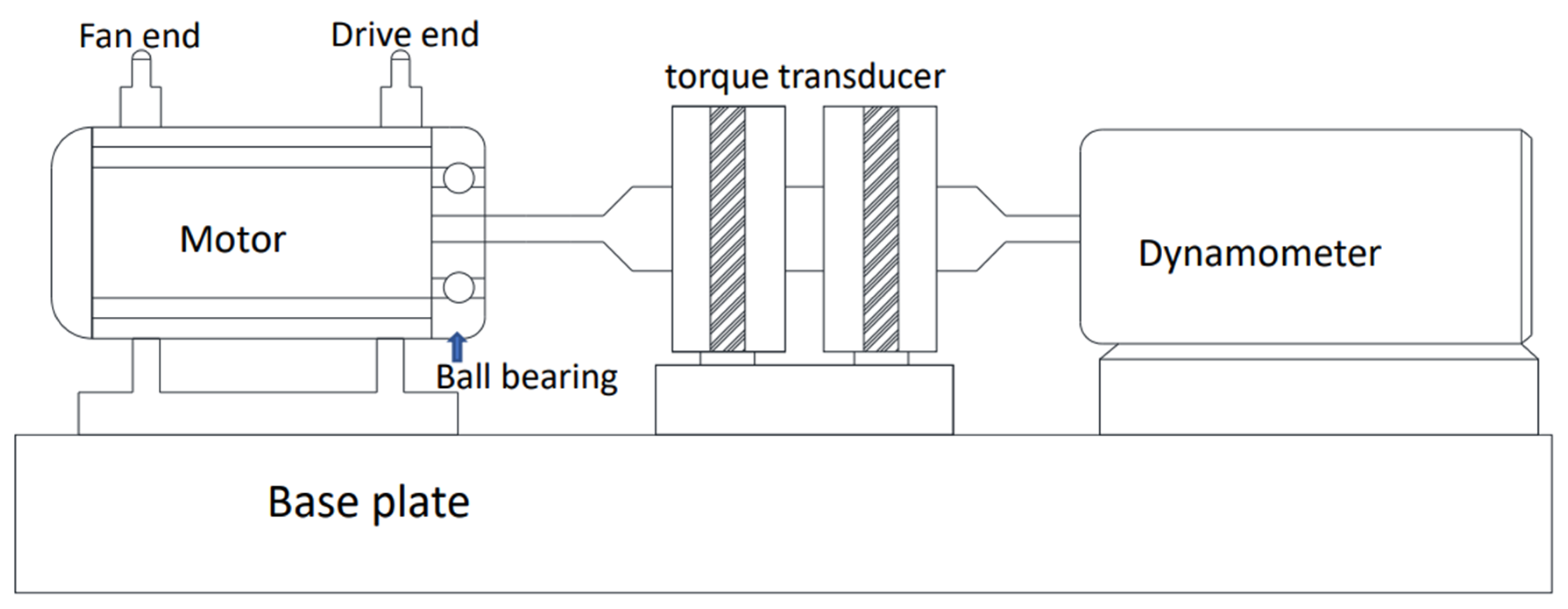
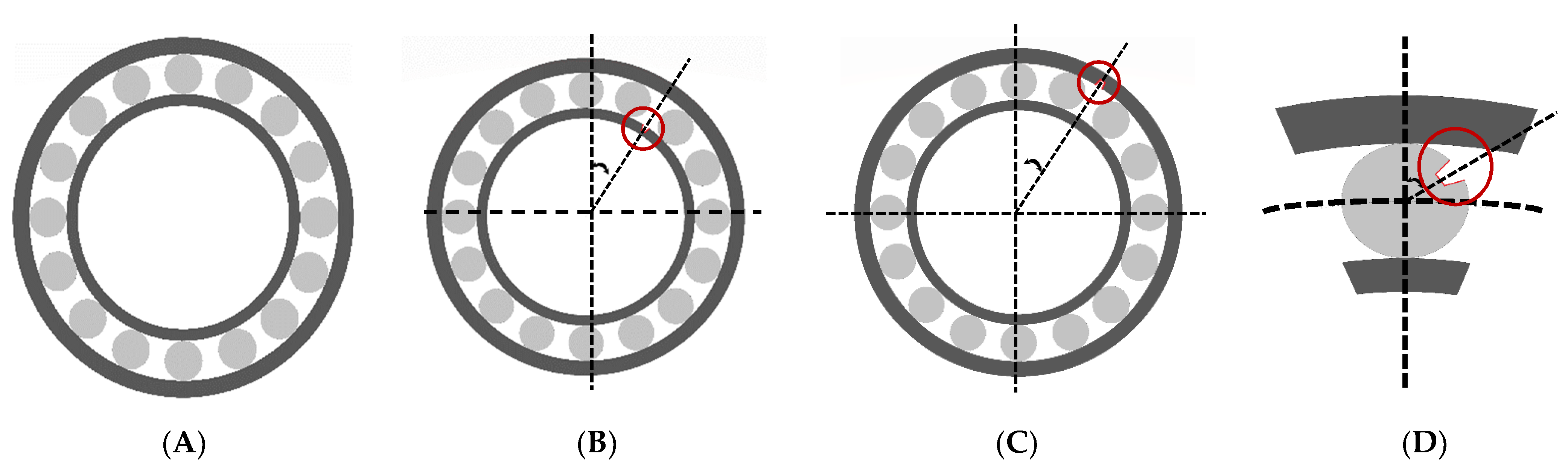
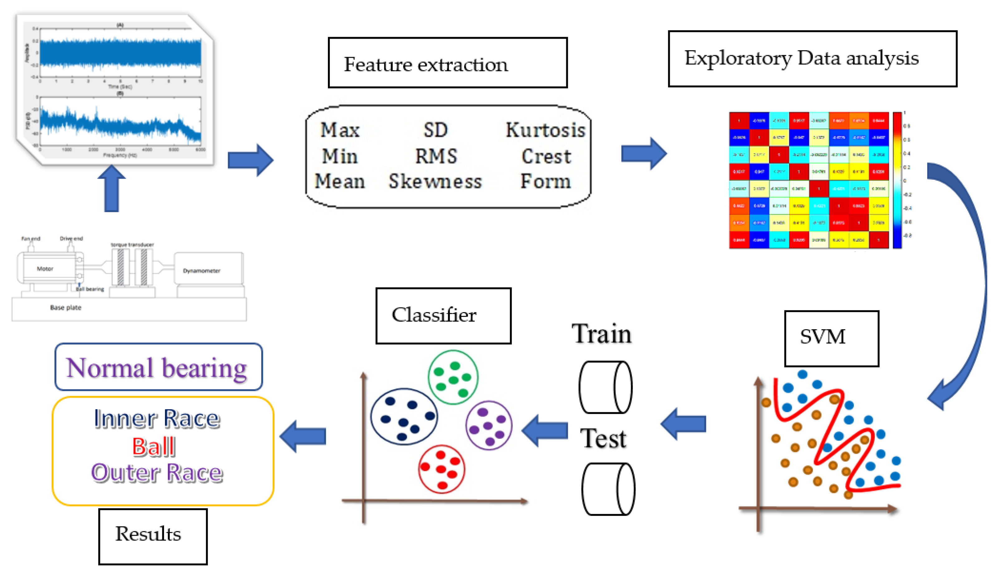
The data obtained from this study, providing test data of normal bearings and faulty bearings of the motor, are based on the website of the Case Western Reserve University Bearing Data Center (https://csegroups.case.edu/bearingdatacenter/home (accessed on 15 September 2021)). Experiments were performed using a motor, and acceleration data were measured near and far from the motor bearing. The web pages on the above website are unique because the actual test conditions of the motor and the bearing failure status are carefully recorded for each experiment. Electrical discharge machining was used to diagnose faults in motor bearings. Faults with diameters ranging from 0.007 inches (0.178 mm) to 0.028 inches were introduced on the inner race, the rolling element (sphere), and the outer race. The faulty bearings were reinstalled into the test motor, and the vibration data of the motor load of 0–3 horsepower (motor speed 1720–1797 rpm) were recorded. As shown in Figure 1, the test bench consisted of a one-horsepower motor (left), a torque sensor/encoder (center), a dynamometer (right), and control electronics (not shown). For 0.007, 0.0014, and 0.0021-inch diameter failures, SKF bearings were used, and for 0.0028-inch failures, NTN equivalent bearings were used. Vibration data were collected using an accelerometer, connected to a housing with a magnetic base. The accelerometer was placed at the 12 o′clock position of the drive end and the fan end of the motor housing. A 16-channel DAT recorder was used to collect the vibration signal, and post-processing was performed in the MATLAB environment. For drive-end bearing failures, 48,000 samples/s were collected. Table 1 shows the electric motor failure conditions, the load, and speed records. There were three types of bearing failure items: the inner race, the ball, and the outer race. Each fault item had three fault diameters: 0.007, 0.0014, and 0.0021 inches. According to the fault situation, the nine categories were represented as Ball_007, Ball_014, Ball_021, IR_007, IR_014, IR_021, OR_007, OR_014, and OR_021, in addition to ten categories of normal bearings. There were 230 test data in each of the above categories, totaling 2300 test data. Figure 2 shows a schematic definition of the processing failure of the bearing. Figure 3. Shows a flowchart describing the SVM method.
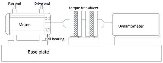
Figure 1.
Experimental platform of the CWRU bearing test rig for a ball bearing system.

Table 1.
Electric motor fault condition and load and speed record on the drive end.
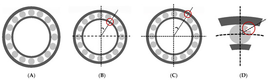
Figure 2.
Bearing conditions: (A) normal; (B) inner race failure; (C) outer race failure; (D) ball failure.
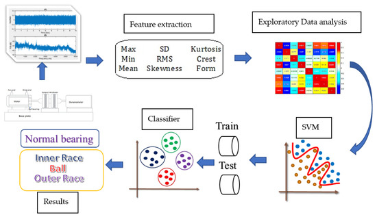
Figure 3.
Flowchart to describe the SVM method.
The original data of the vibration signal of a motor are generally in the time waveform, and their time-domain waveform is intuitive and easy to understand. Therefore, when the fault signal waveforms, such as unbalance, misalignment, and impact, have obvious characteristics, the time domain waveforms are often used for analysis first. At the same time, the time domain waveform, as the most primitive signal of vibration analysis, provides the truest and most comprehensive information and does not lose information due to transformation, such as spectrum analysis. Therefore, in fault analysis and diagnosis, the combination of spectrum analysis and time-domain waveform analysis makes the diagnosis result more accurate. The time-domain analysis is the most basic part of signal processing. The principle is simple and easy to implement. It mainly includes time-domain waveforms, probability density, correlation analysis, filter processing, etc. Time-domain analysis has a wide range of applications, especially for some low-speed, variable-speed, and heavy-duty equipment. Due to the low-frequency components contained in the vibration signal, time-domain analysis is limited by the lower limit of the vibration diagnostic analysis instrument, the resolution, and the analysis software function. The results of the analysis are not ideal. The time-domain analysis is one of the most effective and direct fault diagnosis methods to easily extract the characteristics of the vibration signal. Fast Fourier transform (FFT) is a mathematical method for converting time-domain waveforms into frequency-domain spectrum graphs. Generally, more information about the data can be obtained through FFT. The number of vibrations per unit time is called frequency. For the number of vibrations per second, the unit is hertz. The highest (low) distance of vibration is called amplitude. The starting point of the vibration is called phase. As the vibration measurement data are discrete, they are generally represented by the following equation using discrete Fourier [50,51]:
Here, represents the vibration measurement data, and N is the length of the data. The motor load was 1 HP, the motor speed was 1772 rpm, the bearing manufacturer was SKF, the sampling time was 10 s, and the sampling frequency was 48,000 Hz. The fault diameter was 0.007″, the tooth depth was 0.011, the motor load was 1 HP, the motor speed was 1772 rpm, the bearing manufacturer was SKF, the sampling time is 10 s, and the sampling frequency was 48,000 Hz. The fault diameter was 0.007″, the tooth depth was 0.011, the motor load was 1 HP, the motor speed was 1772 rpm, the bearing manufacturer was SKF, the sampling time was 10 s, and the sampling frequency was 48,000 Hz. The fault diameter was 0.007″, the tooth depth was 0.011, the motor load was 1 HP, the motor speed was 1772 rpm, the bearing manufacturer was SKF, the sampling time was 10 s, and the sampling frequency was 48,000 Hz. The most commonly used vibration data are obtained from time domain and frequency domain analysis methods. As this study could not obtain good results using the time and frequency domains, a Gaussian SMV was used.
Correlation analysis is one of the basic methods of vibration signal processing. It uses statistics, such as correlation coefficient, correlation function, and correlation coefficient function, to study and describe the correlation between vibration signals in engineering. This study mainly introduces the most used related functions. Correlation functions were divided into auto- and cross-correlation functions. According to Equations (12)–(17), the following nine features were calculated for fault identification prediction: maximum value, minimum value, average value, standard deviation, RMS, skewness, kurtosis, crest factor, and form factor. As the standard deviation was the same as the RMS, the standard deviation was used. There were 230 test data in each of the categories; a total of 2300 test data were in the correlation analysis. Table 2 shows the 9 features calculated in the original vibration data for the 10 categories of labels, with 230 labels for each category and a total of 2300 data.
Table 2.
There are 9 features calculated in the original vibration data for 10 categories of labels, 230 labels for each category, a total of 2300 data.
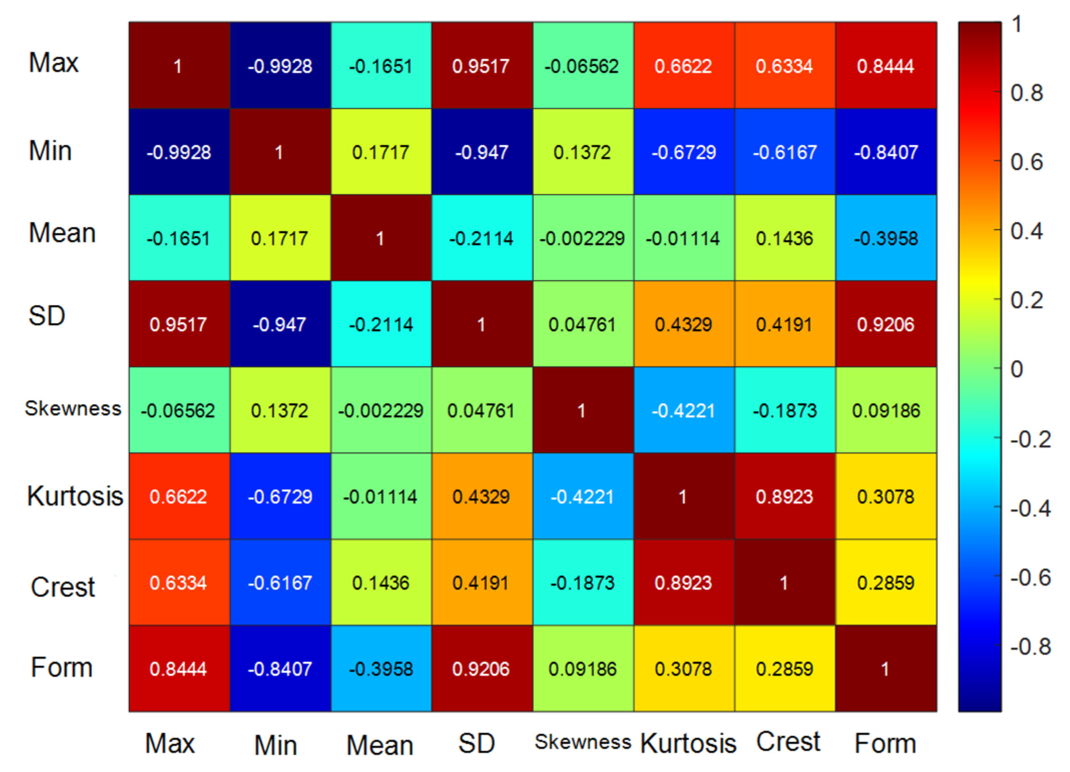
Figure 4 shows that the correlation matrix had eight features; 1 indicated positive correlation, and −1 indicated negative correlation. The negative correlation coefficient of the maximum and minimum features was −0.9928; the positive correlation coefficient of the maximum, SD, and RMS features was 0.9517; and the negative correlation coefficients of the minimum, maximum, and SD features were −0.9928, −0.947, and −0.947, respectively. The mean feature had a low correlation with other features. The positive correlation coefficients of the SD, maximum, and form factor features were 1, 0.9517, and 0.9206, respectively. The positive correlation coefficients of the SD, maximum, and form factor features were 1, 0.9517, and 0.9206, respectively. Skewness, kurtosis, and crest features had a low correlation with other features. The positive correlation coefficient of the form factor, SD, and RMS features was 0.9206, and they had a low correlation with other features.
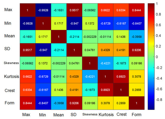
Figure 4.
The correlation matrix had eight features.
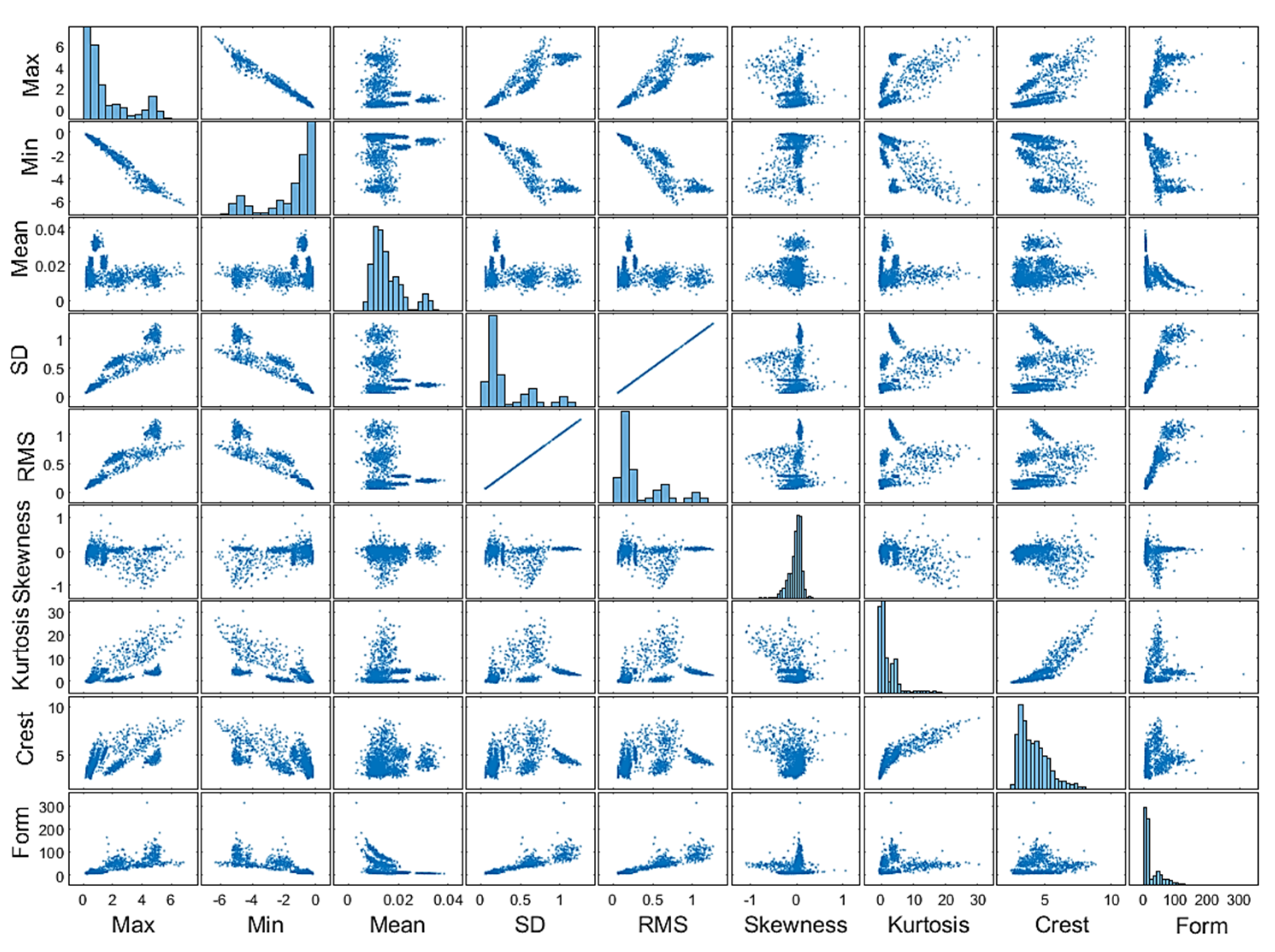
Correlation is also called association. In probability theory and statistics, correlation shows the strength and direction of the linear relationship between two or several random variables. In statistics, the significance of correlation is that it is used to measure the distance between two features relative to their mutual independence. Correlation coefficients are usually used to measure the degree of synergistic changes in these characteristics. When the characteristics show a trend of change in the same direction, the correlation is positive; otherwise, it is negative. Figure 5 shows the distribution of the scatter diagram of the nine features of the correlation matrix. A scatter diagram shows the distribution of two variables in data. Each point represents the value of a feature, and its coordinates on the horizontal and vertical axes correspond to the feature of the data. There were 230 test data in each of the nine features, and a total of 2300 test data were in the analysis. After each test datum was calculated using Equations (12)–(17), nine feature values were obtained. A 9 × 230 matrix was obtained for each category, and a 9 × 2300 matrix was obtained for the nine features. Figure 5 was obtained by using the scatter diagram. The scatter diagram and correlation had three characteristics as follows:
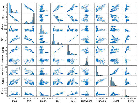
Figure 5.
The correlation matrix is the distribution of the scatter diagram of nine features.
- Positive correlation scatter diagram: When the slope of the data distribution is positive, the correlation is positive, that is, the two variables have a consistent trend (increasing or decreasing at the same time);
- Negative correlation scatter diagram: When the slope of the data distribution is negative, the correlation is negative, that is, when one increases, the other decreases, and vice versa;
- Zero correlation scatter diagram: A change in one variable has no effect on the other. When the scattered points are symmetrical up, down, left, and right or when the points are completely distributed along a straight line parallel to the x- or the y-axis, the two variables are said to have zero correlation.
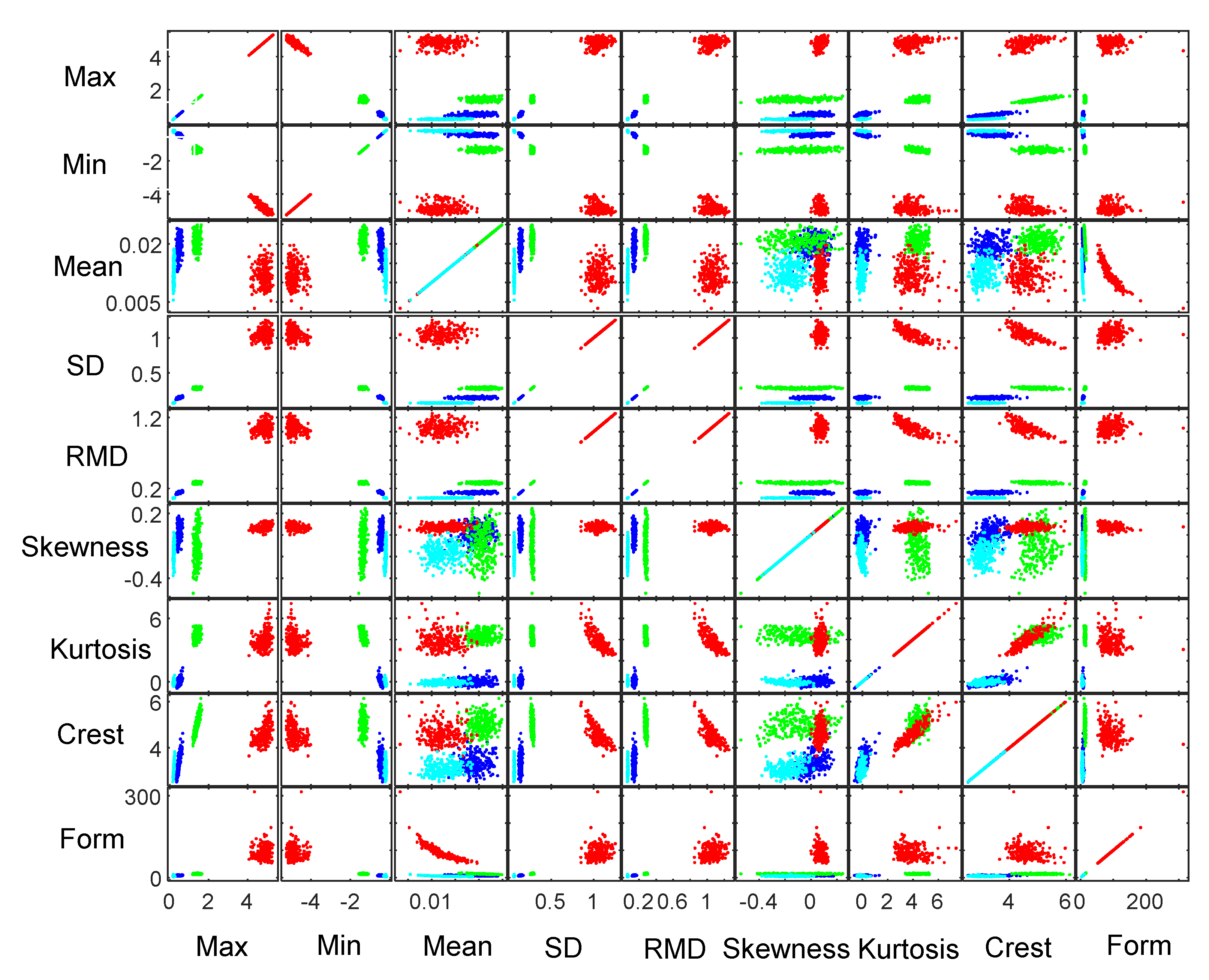
The more separated the data of each category are, the easier it is to classify the data in the scatter diagram, but the classification could not be displayed in Figure 5. Therefore, in Figure 6, there are four categories: normal (light blue), ball (blue), inner ring (green), and outer ring (red). Figure 6 shows that the plot matrix created a sub-axis matrix containing row scatter plots of the nine features, which are located on the motor bearing faulty ball (blue), the inner ring (green), the outer ring (red), and normal (light blue) categories. Figure 5 does not show the correlation of the classification situation. Figure 6 shows the correlation of the four categories. If the data distribution is more scattered, it means that the features are easier to separate.
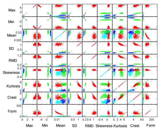
Figure 6.
The plot matrix creates a sub-axis matrix of row scatter plots of nine features in the motor bearing failure ball (blue), the inner race (green), the outer race (red), and normal (light blue) categories.
The SVM uses a hyperplane to cut data belonging to two different categories. The SVM can obtain a set of parameter-adjusted models from the training data set and use the trained models to predict the category of unclassified data.
The confusion matrix is an indicator of the fault diagnosis and a prediction classification model. The more accurate the confusion matrix, the better. Therefore, corresponding to the confusion matrix, the number of TPs and TNs should be large and the number of FPs and FNs small. However, there can never be a perfect system, so FPs and FNs will appear. Therefore, in a confusion matrix of a model, it is necessary to see how many observations are in positions corresponding to the second and fourth quadrants. The more values in these quadrants, the better. In contrast, the fewer observations in the first and third quadrants, the better. This study used nine features, each with 230 test data, and a total of 2300 test data were analyzed. To obtain the maximum amount of evaluation data, no training test was performed after the establishment of the SVM model, because the training data could not be evaluated. Therefore, the nine features were directly evaluated and verified with a total of 2300 test data. The same results could be obtained by repeating this study 100 times. This method directly takes the original signal as input and realizes end-to-end diagnosis through nine features. SVM is a supervised algorithm. In model evaluation, the label is a very important key role in the supervision algorithm, so the research needs to know the label of the target. Health is a normal motor bearing. There are three types of faulty motor bearings. The first type is a bearing ball failure such as Ball_007, Ball_014, Ball_021. The second type is the bearing inner ring fault such as IR_007, IR_014, IR_021. The third type is the bearing outer ring failure such as OR_007, OR_014, OR_021. Therefore, there are nine categories of faults in the data. In addition, 007, 014, 021 represent the diameter of the fault crack of the bearing in inches. These codenames represent the fault category and label discussed in the results. Figure 7 shows the confusion matrix for the failure prediction of motor bearings. There were three types of failure modes (ball, inner race, and outer race), and each type of fault crack was 0.007, 0.014, and 0.021 inches, so there was a total of nine categories, plus a normal bearing, amounting to ten categories in the confusion matrix. On the right side of Figure 7, the true-positive rate (TPR) and false-positive rate (FPR) are shown. TPR stands for prediction accuracy, and the higher it is, the better. FPR stands for prediction error, and it is as low as possible.
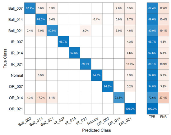
Figure 7.
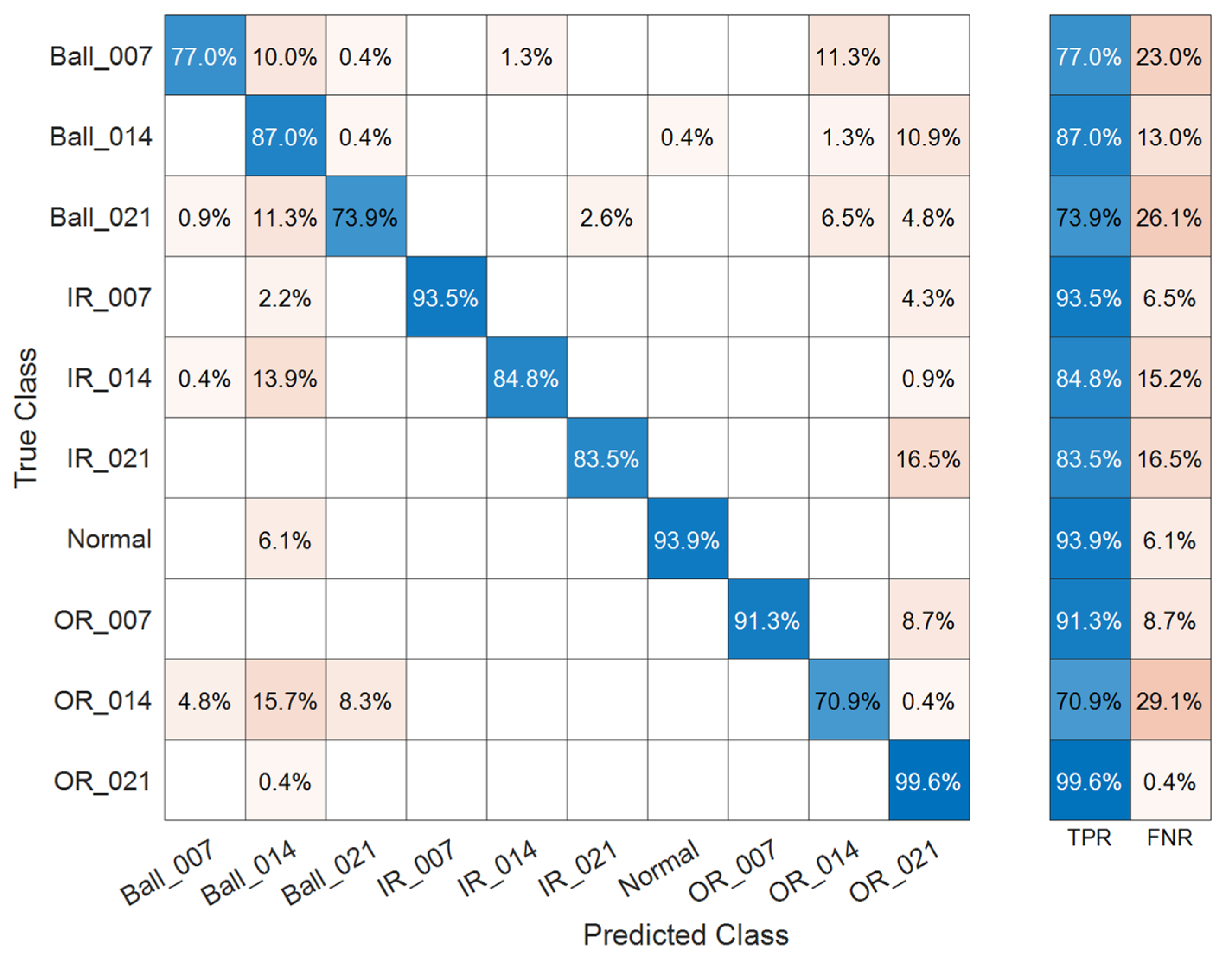
Confusion matrix of motor bearing failure prediction in fine Gaussian SVM, with a total accuracy of 89.6%.
Here, in particular, the novelty of the proposed method in this study is discussed, and its performance is compared with the existing methods. First, Figure 7 shows the confusion matrix of the motor bearing fault prediction in the fine Gaussian SVM. Through the fine Gaussian SVM model, the TP of Ball_007 was predicted to be 87.4%. In addition, Ball_014 had an error prediction of 3.0%, Ball_021 1.3%, and OR_014 4.8%, OR_014 3.5%, and the total error prediction was 12.6%. The total accuracy of motor bearing fault prediction in fine Gaussian SVM was 89.3%.
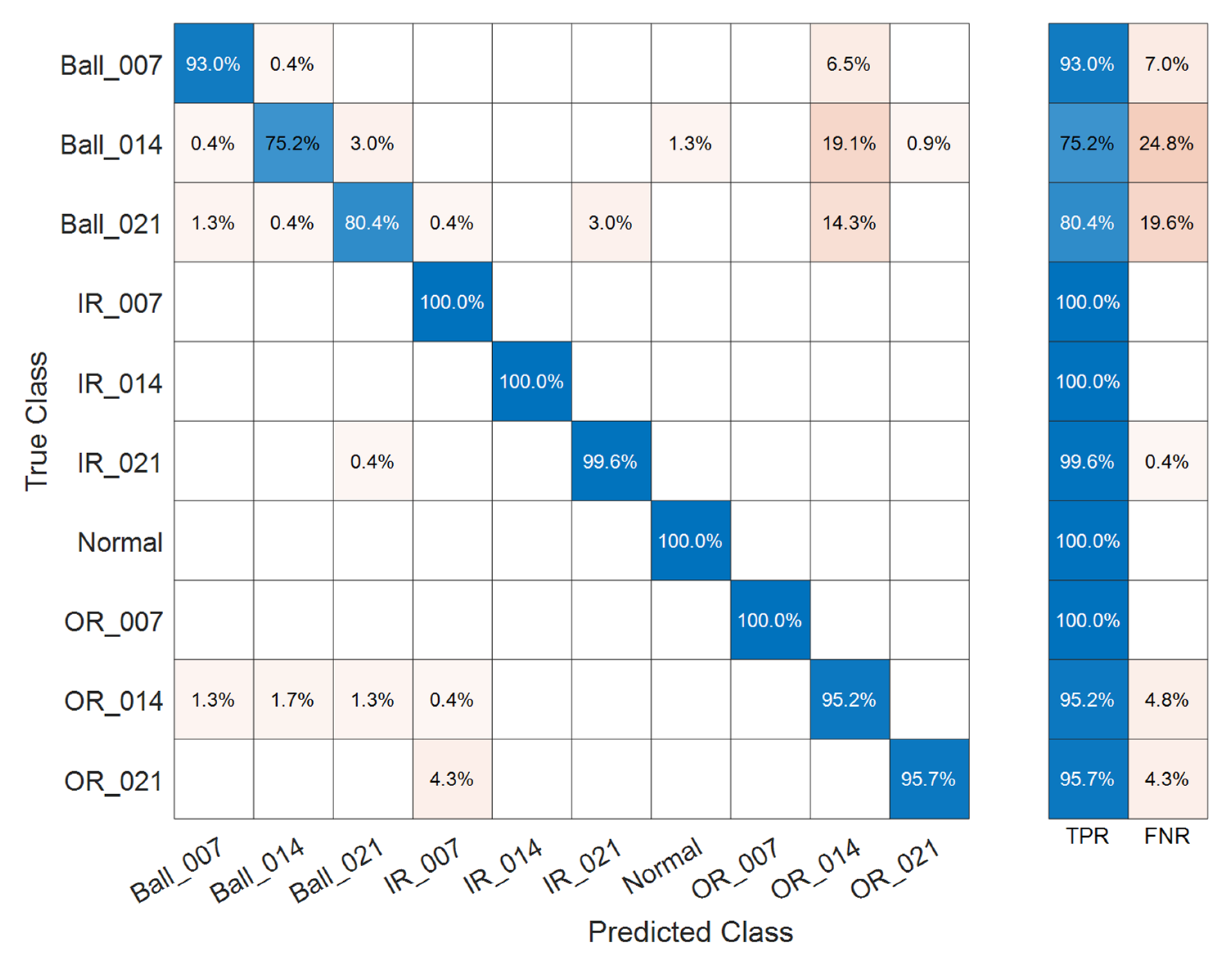
Figure 8 shows the confusion matrix of the motor bearing fault prediction in the coarse Gaussian SVM. Through the coarse Gaussian SVM model, the TP of Ball_007 was predicted to be 93.0%. In addition, Ball_014 had an error prediction of 0.4%, OR_014 6.5%, and the total error prediction was 7.0%. The total accuracy of motor bearing fault prediction in coarse Gaussian SVM was 93.6%.
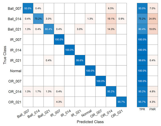
Figure 8.
Confusion matrix of motor bearing failure prediction in coarse Gaussian SVM, with a total accuracy of 93.6%.
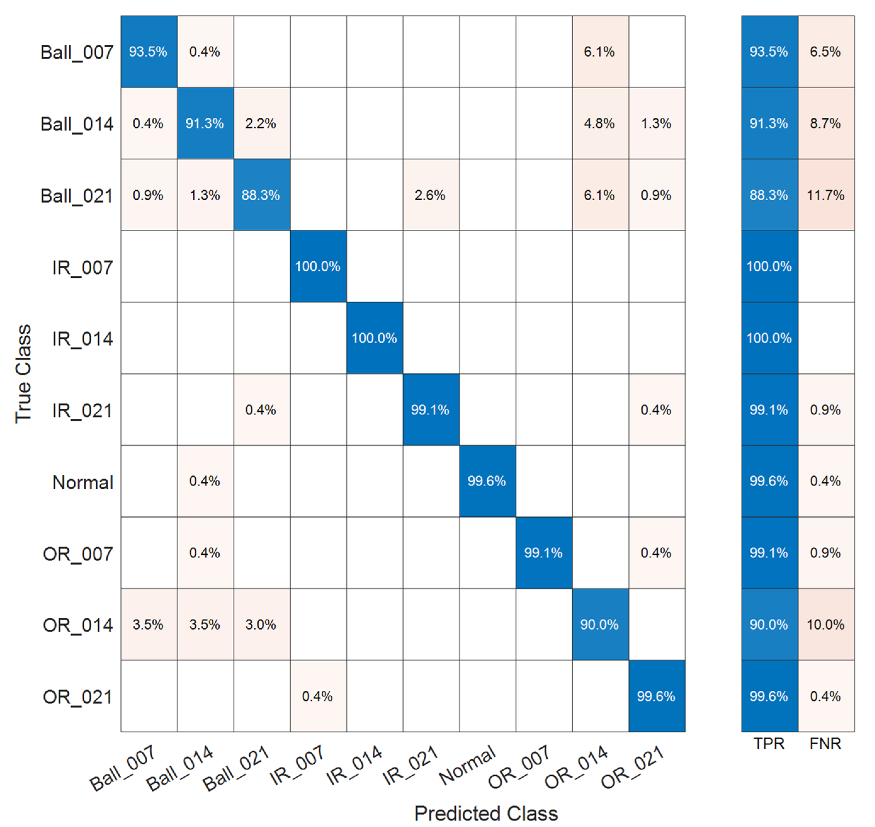
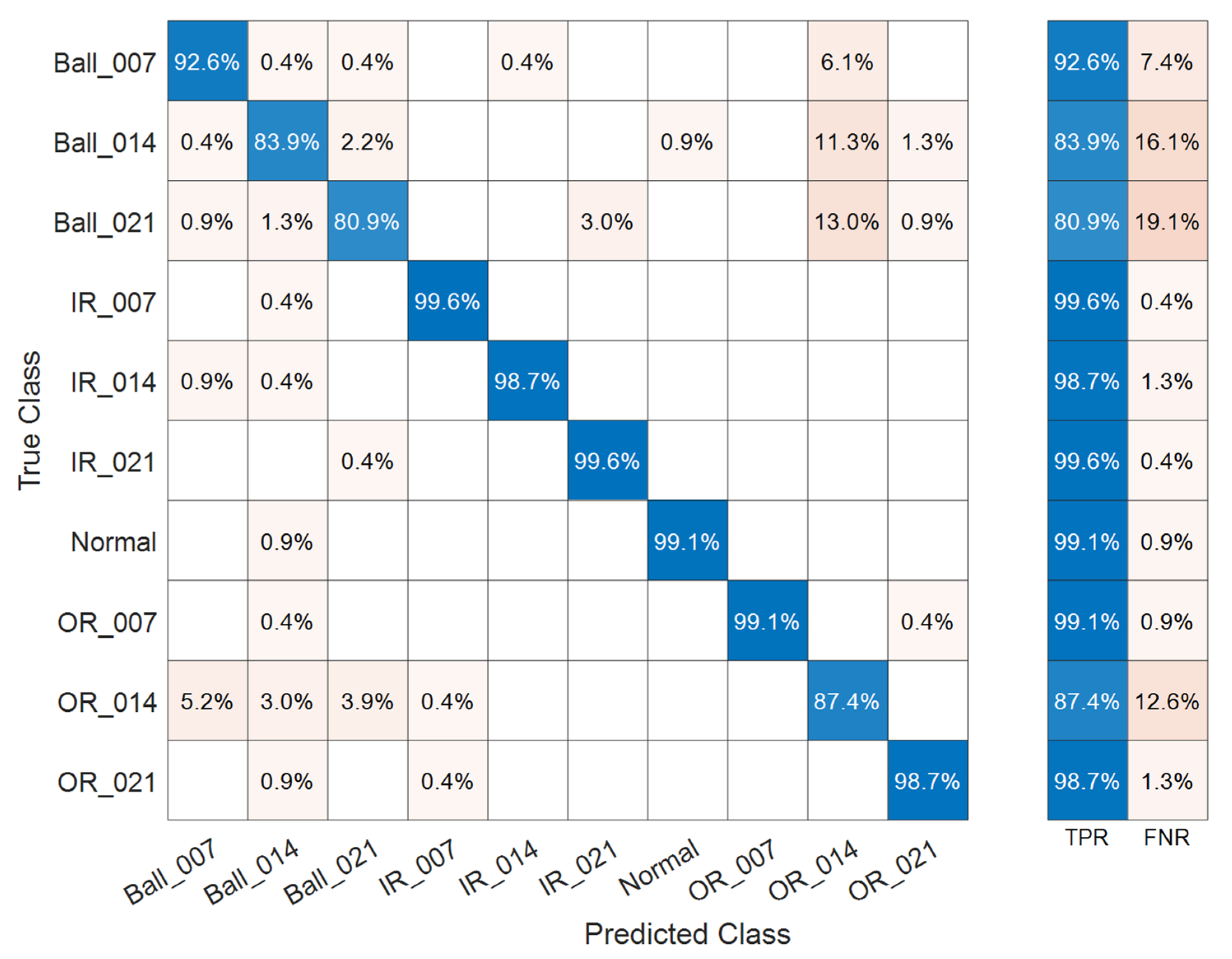
Figure 9 shows the confusion matrix of the motor bearing fault prediction in the medium Gaussian SVM. Through the medium Gaussian SVM model, the TP of Ball_007 was predicted to be 93.5%. In addition, Ball_014 had an error prediction of 0.4%, OR_014 6.1%, and the total error prediction was 6.5%. The total accuracy of motor bearing fault prediction in medium Gaussian SVM was 96%.
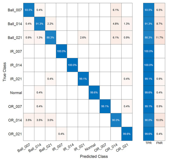
Figure 9.
Confusion matrix of motor bearing failure prediction in medium Gaussian SVM, with a total accuracy of 96%.
This study used Gaussian kernels of different sizes in fine, medium, and coarse Gaussian SVMs. This method can classify more complex data. The relevant characteristics are described below. A fine Gaussian SVM uses a Gaussian kernel. The kernel scale is 𝑠𝑞()/4 as in Equation (12), where is the number of features that can achieve a fine distinction between categories. The prediction speed is fast in binary and slow in multiple categories. Memory usage is medium in binary and large in multiple categories. Interpretability is difficult. The flexibility of the model is high and decreases with the setting of the nuclear scale. For a fine distinction between classes, the kernel ratio was set to sqrt()/4. The accuracy of the prediction was 89.6%.
Finally, the coarse Gaussian SVM uses a Gaussian check to make a rough distinction. The kernel scale is as in Equation (12). According to different classification data characteristics, there are different Gaussian kernel applications. The prediction speed is fast in binary and slow in multiple categories. Memory usage is medium in binary and large in multiple categories. Interpretability is difficult. The flexibility of the model is high and decreases with the setting of the nuclear scale. A fine distinction between classes is a low-level distinction. The accuracy of the prediction was 93.6%.
The medium Gaussian SVM has fewer distinctions between classes, and it also uses Gaussian kernels. The kernel scale used is 𝑠𝑞() as in Equation (12). The prediction speed is fast in binary and slow in multiple categories. Memory usage is medium in binary and large in multiple categories. Interpretability is difficult. The flexibility of the model is high and decreases with the setting of the nuclear scale. For a fine distinction between classes, the nuclear scale was set to sqrt(). The accuracy of the prediction was 96%.
As there is often noise interference in the actual application environment, in order to verify the performance of the research method in a noisy environment, simulated Gaussian white noise was added to the signal. In general, the traditional preprocessing filters, such as low-pass filter, high-pass filter, bandpass filter, and band-reject filter, are first used. The purpose of the filter is to pass signals in a specific frequency band and then attenuate all signals outside this frequency band. In other words, it is necessary to know which are the main frequencies to be left, and which are the noise frequencies to be filtered. However, many noises are broadband and cannot be preprocessed with traditional filters. Noise interference will affect classification performance and reduce classification accuracy. The test results are under the same standard and fair conditions in a noisy environment. To simulate Gaussian white noise, set the parameter mean value parameter to 0, and the random number of the standard deviation parameter to 0.1. Figure 10, Figure 11 and Figure 12 show the confusion matrix and total accuracy of the motor bearing fault prediction in the three SVMs under noisy environments. The research results show that the 94% accuracy rate of the intelligent diagnosis method using the medium Gaussian SVM is better than the 85.5% accuracy rate of the fine Gaussian SVM and the 88.3% accuracy rate of the coarse Gaussian SVM. Compared with a noisy environment, the medium Gaussian SVM is reduced by 2%, the fine Gaussian SVM is reduced by 4.1%, and the coarse Gaussian SVM is reduced by 5.3%. The medium Gaussian SVM obtains better performance than the other two methods in a noisy environment. The main noise will interfere with the real data, and it will cause errors between the features and the real data during feature extraction. For example, the RMS is 0.5 when there is no noise interference, and the RMS is 0.6 after noise interference, which will cause all nine characteristics to be affected. There are 10 types of label classification. When noise will interfere with different types of features that are close or overlapped, the accuracy of SVM classification will decrease. This study found that the larger the noise standard deviation parameter is, the more the accuracy of SVM classification will decrease. Table 3 shows that the noise level affects the comparison of the accuracy of the three SVM results. This result shows the robustness of the proposed method and is not easily affected by noise interference.
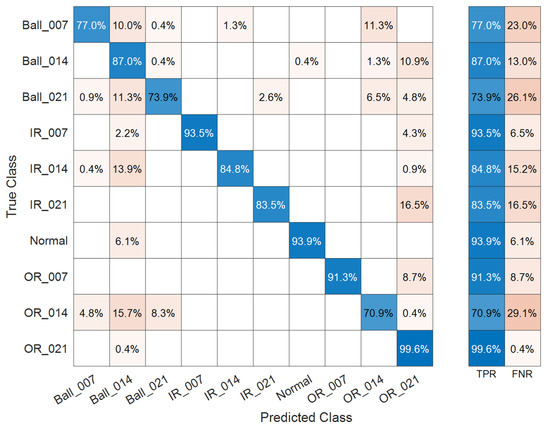
Figure 10.
Confusion matrix of motor bearing failure prediction in fine Gaussian SVM on the noisy environment, with a total accuracy of 85.5%.
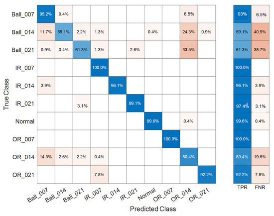
Figure 11.
Confusion matrix of motor bearing failure prediction in coarse Gaussian SVM on the noisy environment, with a total accuracy of 88.3%.

Figure 12.
Confusion matrix of motor bearing failure prediction in medium Gaussian SVM on the noisy environment, with a total accuracy of 94%.
Table 3.
The noise level affects the comparison of the accuracy of the three SVM results.
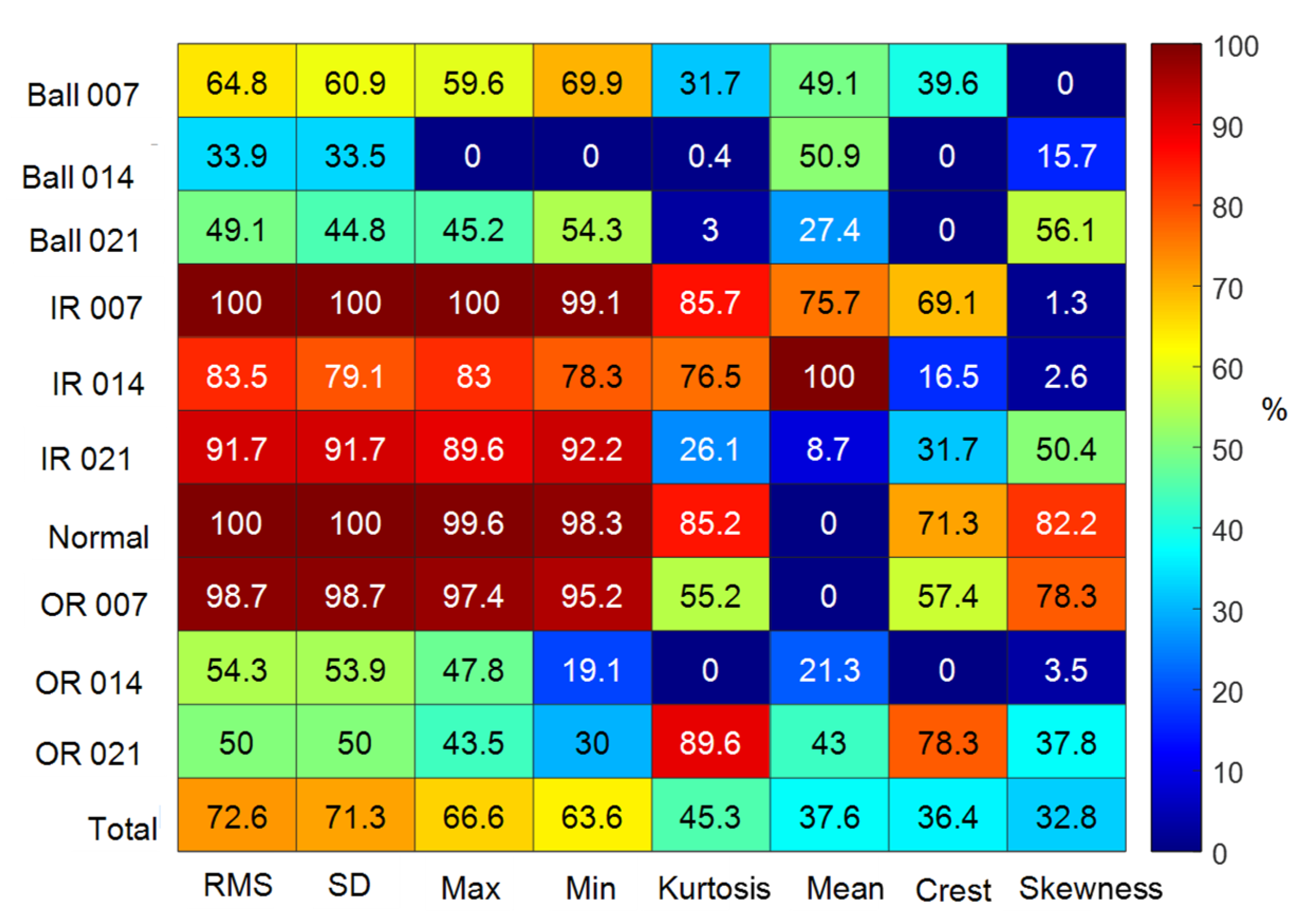
All these research results used nine features. In this part of the study, the focus was on understanding which feature is the most important. Therefore, as shown in Figure 13, only one feature was used to predict the results. In the results predicted only by RMS, IR_007 and the normal bearing reached 100%, the worst case was 33.9% of Ball_014, and the sum of all predictions showed an accuracy of 72.6%. In the results predicted using only the SD feature, IR_007 and the normal bearing reached 100%, the worst case was 33.5% of Ball_014, and the sum of all predictions showed an accuracy of 71.3%. In the results predicted using only the maximum feature, IR_007 reached 100%, the normal bearing reached 99.6%, the worst case was 0% of Ball_014, and the sum of all predictions showed an accuracy of 66.6%. In the results predicted using only the minimum feature, IR_007 reached 99.1%, the normal bearing reached 98.3%, the worst case was 0% of Ball_014, and the sum of all predictions showed an accuracy of 63.6%. In the results predicted using only kurtosis, OR_021 reached 89.1%, the normal bearing reached 85.2%, the worst case was 0% of OR_014, and the sum of all predictions showed an accuracy of 45.3%. In the results predicted using only the mean, IR_014 reached 100%, the worst case was the normal bearing and 0% of OR_007, and the sum of all predictions showed an accuracy of 37.6%. In the results predicted using only the crest feature, the normal bearing reached 71.3%, the worst case was 0% of Ball_014, Ball_021, and OR_021, and the sum of all predictions showed an accuracy of 36.4%. In the result predicted using only the skewness feature, the normal bearing reached 82.2%, the worst case was 0% of Ball_007, and the sum of all predictions showed an accuracy of 32.8%. Therefore, when only one feature was used for prediction, the most important feature was the RMS, and an accuracy rate of 72.6% could be obtained. The second most important feature was the SD, with an accuracy rate of 71.3%. The accuracy of the mean and crest features was only 36.4% and 32.8%, respectively, and therefore, these are not important when using only one feature to predict.

Figure 13.
Results of predicting motor bearing failure with only one feature.
4. Conclusions
Motor monitoring data analysis has progressed from diagnostic, preventive, and predictive analysis to prognostic analysis. A running motor produces progressive parameter values. When the motor produces failure signs in the early stages, maintenance can be carried out in advance, greatly reducing the cost of equipment failure. With a focus on the problem that the generalization ability of the diagnostic model decreases due to the variable working conditions of the motor, this paper proposed a rolling motor bearing cross-domain fault diagnosis method based on a medium Gaussian SVM. This method directly uses the original signal as the input to realize an end-to-end diagnosis. In model evaluation, this method needs to know the target domain′s label in advance and realizes supervised domain adaptation. The contribution of this study is a detailed literature analysis and characteristic discussion of the bearing failure data of electric motors. In the analysis results, the time domain and frequency domain, correlation analysis, and feature analysis were also used to analyze the characteristics of the faulty bearing in detail. This research discusses r as a parameter of the kernel. In practical applications, this research found that it is very effective in classification results. In general cases, the coarse Gaussian kernel has good performance, so it is currently the most widely used kernel function. However, with the continuous exploration of research work and the promotion of applied research, there are more and more choices of kernel functions for different problems. The study found that the medium Gaussian has a better classification result in the fault diagnosis of the motor. This study compared the performance of different Gaussian kernels through the data set released by the Bearing Data Center of Case Western Reserve University. Experimental results show that the 96% accuracy of the medium Gaussian SVM intelligent diagnosis method in the use of nine features of motor bearings is better than the 89.6% accuracy of the fine Gaussian SVM and the 93.6% accuracy of the coarse Gaussian SVM. Of the nine features of the motor bearing, the prediction accuracy rate is 72.6% when only the RMS feature is used, and 71.3% when only the SD feature is used. However, the current database only has 9 categories of motor fault data (IR007, IR014, IR021, B007, B014, B021, OR007, OR014, OR021) plus 10 categories of normal. Therefore, the limitation of this study is that these 10 categories can be classified, and fault characteristics beyond these 9 categories will be classified incorrectly. Overall, the method proposed in this paper can effectively realize the cross-domain fault diagnosis of bearings and improve the feasibility of applying the cross-domain diagnosis model in actual industrial scenarios. The proposed strategy can be used to automatically identify machine failures, which will help provide early warnings to avoid unexpected and unplanned system downtime due to bearing failures. SVM is supervised learning and has its limitations. It must have a database of features and labels, that is, the fault category in the training database, in order to be correctly judged. If it is not in the training database, the fault category will be misclassified into other categories. In the future, we plan to build an electric vehicle motor predictive diagnosis system so that the currently designed model can be optimized and self-adjusted in different applications to improve the efficiency of the motor and reduce the loss and safety issues caused by temporary failures. At present, this research aims at the diagnosis of normal health, inner ring defect, outer ring defect, and ball-defect-bearing fault diagnosis. After collecting more database data in the future, it will be possible to diagnose more bearing problems that often occur, such as bearing corrosion or lubricant problems. Future research can add Gaussian SVM to compare with other types of existing meta-models such as ensemble methods, neural networks, or deep learning methods.
Funding
The author would like to thank the Ministry of Science and Technology, Taiwan, for financially supporting this research (Grant No. MOST 109-2222-E-230-001-MY2).
Institutional Review Board Statement
Not applicable.
Informed Consent Statement
Not applicable.
Data Availability Statement
Not applicable.
Acknowledgments
The authors thank Case Western Reserve University for providing free access to the bearing vibration experimental data on their website.
Conflicts of Interest
The author declares no conflict of interest.
References
- Johnson, R.A. An Information Theory Approach to Diagnosis. IRE Trans. Reliab. Qual. Control. 1960, RQC-9, 35. [Google Scholar] [CrossRef]
- Preparata, F.P.; Metze, G.; Chien, R.T. On the Connection Assignment Problem of Diagnosable Systems. IEEE Trans. Electron. Comput. 1967, EC-16, 848–854. [Google Scholar] [CrossRef] [Green Version]
- Sohre, J. Operating problems with high-speed turbomachinery-causes and correction. In Proceedings of the ASME Petroleum Mechanical Engineering Conference, Dallas, TX, USA, 1968. [Google Scholar]
- Sohre, J. Trouble-shooting to stop vibration of centrifugal. Petrop. Chem. Eng. 1968, 11, 22–23. [Google Scholar]
- Jackson, C.; Primer, A.P.V. The Practical Vibration Primer; Gulf Publishing Company: Houston, TX, USA, 1979. [Google Scholar]
- Achenbach, J.D. Structural health monitoring–What is the prescription? Mech. Res. Commun. 2009, 36, 137–142. [Google Scholar] [CrossRef]
- Nair, K.K.; Kiremidjian, A.S.; Law, K.H. Time series-based damage detection and localization algorithm with application to the ASCE benchmark structure. J. Sound Vib. 2006, 291, 349–368. [Google Scholar] [CrossRef]
- Park, S.; Yun, C.-B.; Roh, Y.; Lee, J.-J. PZT-based active damage detection techniques for steel bridge components. Smart Mater. Struct. 2006, 15, 957–966. [Google Scholar] [CrossRef]
- Takeda, N.; Okabe, Y.; Mizutani, T. Damage detection in composites using optical fibre sensors. Proc. Inst. Mech. Eng. Part G J. Aerosp. Eng. 2007, 221, 497–508. [Google Scholar] [CrossRef]
- Albarbar, A.; Mekid, S.; Starr, A.; Pietruszkiewicz, R. Suitability of MEMS Accelerometers for Condition Monitoring: An experimental study. Sensors 2008, 8, 784–799. [Google Scholar] [CrossRef] [PubMed] [Green Version]
- Albarbar, A.; Badri, A.; Sinha, J.K.; Starr, A. Performance evaluation of MEMS accelerometers. Measurement 2009, 42, 790–795. [Google Scholar] [CrossRef] [Green Version]
- Son, J.-D.; Ahn, B.-H.; Ha, J.-M.; Choi, B.-K. An availability of MEMS-based accelerometers and current sensors in machinery fault diagnosis. Measurement 2016, 94, 680–691. [Google Scholar] [CrossRef]
- Bachschmid, N.; Pennacchi, P. Crack effects in rotordynamics. Mech. Syst. Signal Process. 2008, 22, 761–762. [Google Scholar] [CrossRef] [Green Version]
- Gasch, R. Dynamic behaviour of the Laval rotor with a transverse crack. Mech. Syst. Signal Process. 2008, 22, 790–804. [Google Scholar] [CrossRef]
- Chen, P.; Toyota, T.; He, Z. Automated function generation of symptom parameters and application to fault diagnosis of machinery under variable operating conditions. IEEE Trans. Syst. Man Cybern. Part A: Syst. Hum. 2001, 31, 775–781. [Google Scholar] [CrossRef]
- Sekhar, A.S. Multiple cracks effects and identification. Mech. Syst. Signal Process. 2008, 22, 845–878. [Google Scholar] [CrossRef]
- Peng, Z.; Jackson, M.; Rongong, J.; Chu, F.; Parkin, R. On the energy leakage of discrete wavelet transform. Mech. Syst. Signal Process. 2009, 23, 330–343. [Google Scholar] [CrossRef] [Green Version]
- Immovilli, F.; Bellini, A.; Rubini, R.; Tassoni, C. Diagnosis of bearing faults in induction machines by vibration or current signals: A critical comparison. IEEE Trans. Ind. Appl. 2010, 46, 1350–1359. [Google Scholar] [CrossRef]
- Immovilli, F.; Cocconcelli, M.; Bellini, A.; Rubini, R. Detection of Generalized-Roughness Bearing Fault by Spectral-Kurtosis Energy of Vibration or Current Signals. IEEE Trans. Ind. Electron. 2009, 56, 4710–4717. [Google Scholar] [CrossRef]
- Chen, C.-C.; Liu, Z.; Yang, G.; Wu, C.-C.; Ye, Q. An Improved Fault Diagnosis Using 1D-Convolutional Neural Network Model. Electronics 2020, 10, 59. [Google Scholar] [CrossRef]
- Ewert, P.; Kowalski, C.T.; Orlowska-Kowalska, T. Low-Cost Monitoring and Diagnosis System for Rolling Bearing Faults of the Induction Motor Based on Neural Network Approach. Electronics 2020, 9, 1334. [Google Scholar] [CrossRef]
- Skowron, M.; Orłowska-Kowalska, T. Efficiency of Cascaded Neural Networks in Detecting Initial Damage to Induction Motor Electric Windings. Electronics 2020, 9, 1314. [Google Scholar] [CrossRef]
- Jardine, A.K.; Lin, D.; Banjevic, D. A review on machinery diagnostics and prognostics implementing condition-based maintenance. Mech. Syst. Signal Process. 2006, 20, 1483–1510. [Google Scholar] [CrossRef]
- Mehrjou, M.R.; Mariun, N.; Marhaban, M.H.; Misron, N. Rotor fault condition monitoring techniques for squirrel-cage induction machine—A review. Mech. Syst. Signal Process. 2011, 25, 2827–2848. [Google Scholar] [CrossRef]
- Gebraeel, N.Z.; Lawley, M.A. A Neural Network Degradation Model for Computing and Updating Residual Life Distributions. IEEE Trans. Autom. Sci. Eng. 2008, 5, 154–163. [Google Scholar] [CrossRef]
- Ihn, J.-B.; Chang, F.-K. Pitch-catch Active Sensing Methods in Structural Health Monitoring for Aircraft Structures. Struct. Heal. Monit. 2008, 7, 5–19. [Google Scholar] [CrossRef]
- Gao, R.X.; Yan, R. Wavelets: Theory and Applications for Manufacturing; Springer: Berlin/Heidelberg, Germany, 2010. [Google Scholar]
- Yan, R.; Gao, R.X. Harmonic wavelet-based data filtering for enhanced machine defect identification. J. Sound Vib. 2010, 329, 3203–3217. [Google Scholar] [CrossRef]
- Gu, F.; Shao, Y.; Hu, N.; Naid, A.; Ball, A. Electrical motor current signal analysis using a modified bispectrum for fault diagnosis of downstream mechanical equipment. Mech. Syst. Signal Process. 2011, 25, 360–372. [Google Scholar] [CrossRef]
- Zhen, D.; Wang, Z.; Li, H.; Zhang, H.; Yang, J.; Gu, F. An Improved Cyclic Modulation Spectral Analysis Based on the CWT and Its Application on Broken Rotor Bar Fault Diagnosis for Induction Motors. Appl. Sci. 2019, 9, 3902. [Google Scholar] [CrossRef] [Green Version]
- Pietrzak, P.; Wolkiewicz, M. On-line Detection and Classification of PMSM Stator Winding Faults Based on Stator Current Symmetrical Components Analysis and the KNN Algorithm. Electronics 2021, 10, 1786. [Google Scholar] [CrossRef]
- Zamudio-Ramirez, I.; Osornio-Rios, R.A.; Antonino-Daviu, J.A.; Cureño-Osornio, J.; Saucedo-Dorantes, J.-J. Gradual Wear Diagnosis of Outer-Race Rolling Bearing Faults through Artificial Intelligence Methods and Stray Flux Signals. Electronics 2021, 10, 1486. [Google Scholar] [CrossRef]
- Chui, K.T.; Gupta, B.B.; Vasant, P. A Genetic Algorithm Optimized RNN-LSTM Model for Remaining Useful Life Prediction of Turbofan Engine. Electronics 2021, 10, 285. [Google Scholar] [CrossRef]
- Kruzic, J.J. Predicting Fatigue Failures. Science 2009, 325, 156–158. [Google Scholar] [CrossRef]
- Heng, A.; Zhang, S.; Tan, C.; Mathew, J. Rotating machinery prognostics: State of the art, challenges and opportunities. Mech. Syst. Signal Process. 2009, 23, 724–739. [Google Scholar] [CrossRef]
- Piltan, F.; Prosvirin, A.E.; Jeong, I.; Im, K.; Kim, J.-M. Rolling-Element Bearing Fault Diagnosis Using Advanced Machine Learning-Based Observer. Appl. Sci. 2019, 9, 5404. [Google Scholar] [CrossRef] [Green Version]
- Chen, Y.; Liang, S.; Li, W.; Liang, H.; Wang, C. Faults and Diagnosis Methods of Permanent Magnet Synchronous Motors: A Review. Appl. Sci. 2019, 9, 2116. [Google Scholar] [CrossRef] [Green Version]
- Dineva, A.; Mosavi, A.; Gyimesi, M.; Vajda, I.; Nabipour, N.; Rabczuk, T. Fault Diagnosis of Rotating Electrical Machines Using Multi-Label Classification. Appl. Sci. 2019, 9, 5086. [Google Scholar] [CrossRef] [Green Version]
- Li, G.; Deng, C.; Wu, J.; Chen, Z.; Xu, X. Rolling Bearing Fault Diagnosis Based on Wavelet Packet Transform and Convolutional Neural Network. Appl. Sci. 2020, 10, 770. [Google Scholar] [CrossRef] [Green Version]
- You, Y.-M. Multi-Objective Optimal Design of Permanent Magnet Synchronous Motor for Electric Vehicle Based on Deep Learning. Appl. Sci. 2020, 10, 482. [Google Scholar] [CrossRef] [Green Version]
- Zhou, K.; Tang, J. Uncertainty quantification in structural dynamic analysis using two-level Gaussian processes and Bayesian inference. J. Sound Vib. 2018, 412, 95–115. [Google Scholar] [CrossRef]
- Li, Y.; Liu, S.; Shu, L. Wind turbine fault diagnosis based on Gaussian process classifiers applied to operational data. Renew. Energy 2019, 134, 357–366. [Google Scholar] [CrossRef]
- Zhou, K.; Tang, J. Structural model updating using adaptive multi-response Gaussian process meta-modeling. Mech. Syst. Signal Process. 2021, 147, 107121. [Google Scholar] [CrossRef]
- Mansouri, M.; Fezai, R.; Trabelsi, M.; Hajji, M.; Harkat, M.-F.; Nounou, H.; Nounou, M.N.; Bouzrara, K. A Novel Fault Diagnosis of Uncertain Systems Based on Interval Gaussian Process Regression: Application to Wind Energy Conversion Systems. IEEE Access 2020, 8, 219672–219679. [Google Scholar] [CrossRef]
- Wang, J.; Zhao, R.; Gao, R.X. Probabilistic Transfer Factor Analysis for Machinery Autonomous Diagnosis Cross Various Operating Conditions. IEEE Trans. Instrum. Meas. 2020, 69, 5335–5344. [Google Scholar] [CrossRef]
- Wang, J.; Liang, Y.; Zheng, Y.; Gao, R.X.; Zhang, F. An integrated fault diagnosis and prognosis approach for pre-dictive maintenance of wind turbine bearing with limited samples. Renew. Energy 2020, 145, 642–650. [Google Scholar] [CrossRef]
- Zhou, K.; Tang, J. Harnessing fuzzy neural network for gear fault diagnosis with limited data labels. Int. J. Adv. Manuf. Technol. 2021, 1–15. [Google Scholar] [CrossRef]
- Savas, C.; Dovis, F. The Impact of Different Kernel Functions on the Performance of Scintillation Detection Based on Support Vector Machines. Sensors 2019, 19, 5219. [Google Scholar] [CrossRef] [Green Version]
- Shawe-Taylor, J.; Cristianini, N. Kernel Methods for Pattern Analysis; Cambridge University Press: Cambridge, UK, 2004. [Google Scholar]
- Winograd, S. On Computing the Discrete Fourier Transform. Math. Comput. 1978, 32, 175–199. [Google Scholar] [CrossRef]
- Wang, Z. Fast algorithms for the discrete W transform and for the discrete Fourier transform. IEEE Trans. Acoust. Speech Signal Process. 1984, 32, 803–816. [Google Scholar] [CrossRef]


Publisher’s Note: MDPI stays neutral with regard to jurisdictional claims in published maps and institutional affiliations. |
© 2021 by the author. Licensee MDPI, Basel, Switzerland. This article is an open access article distributed under the terms and conditions of the Creative Commons Attribution (CC BY) license (https://creativecommons.org/licenses/by/4.0/).