SORT-YM: An Algorithm of Multi-Object Tracking with YOLOv4-Tiny and Motion Prediction

Abstract

Multi-object tracking (MOT) is a significant and widespread research field in image processing and computer vision. The goal of the MOT task consists in predicting the complete tracklets of multiple objects in a video sequence. There are usually many challenges that degrade the performance of the algorithm in the tracking process, such as occlusion and similar objects. However, the existing MOT algorithms based on the tracking-by-detection paradigm struggle to accurately predict the location of the objects that they fail to track in complex scenes, leading to tracking performance decay, such as an increase in the number of ID switches and tracking drifts. To tackle those difficulties, in this study, we design a motion prediction strategy for predicting the location of occluded objects. Since the occluded objects may be legible in earlier frames, we utilize the speed and location of the objects in the past frames to predict the possible location of the occluded objects. In addition, to improve the tracking speed and further enhance the tracking robustness, we utilize efficient YOLOv4-tiny to produce the detections in the proposed algorithm. By using YOLOv4-tiny, the tracking speed of our proposed method improved significantly. The experimental results on two widely used public datasets show that our proposed approach has obvious advantages in tracking accuracy and speed compared with other comparison algorithms. Compared to the Deep SORT baseline, our proposed method has a significant improvement in tracking performance.

1. Introduction

Multi-object tracking (MOT), which aims to assign and maintain a unique ID to each object of interest in a video sequence while predicting the location of all objects, is an essential branch of computer vision tasks. MOT has a vital theoretical research significance and application value. An MOT system with well-behaved performance plays a critical part in visual security monitoring systems, vehicle visual navigation systems, human–computer interaction, etc. [1]. However, as shown in Figure 1, there are many challenges in the actual tracking scenarios that will lead to tracking performance decay, including the interaction between objects, occlusions, the high similarity between different objects, interference of the background, etc. Under these challenges, undesirable errors such as bounding box drift and ID switches are prone to occur, resulting in tracking performance decay. Therefore, this paper aims to propose a robust MOT algorithm in complex scenes.

In recent years, lots of MOT methods appeared to perform the MOT task. Among them, owing to the rapid development of object detection, the tracking-by-detection (TBD) paradigm has shown excellent performance and is the most commonly used framework [2]. As shown in Figure 2, the TBD paradigm consists of a detector and a data association procedure. First, the detector is used to locate all objects of interest from the video sequence. Then, the feature information of each object is extracted in the data association process, and the same objects are associated according to the metrics (e.g., appearance feature and motion feature) defined on the feature. Finally, by associating the same object in different video frames, a continuously updated tracklet set is formed. Obviously, in this TBD paradigm, the performance of the detector and the data association algorithm jointly determine the tracking accuracy and robustness. Undesirable detection results may lead to bounding box drift and low tracking precision. Meanwhile, the performance of the data association has a great impact on some vital metrics such as the number of ID switches, tracklet segmentation, etc. In addition, both the detector and the data association greatly influence the inference speed of the MOT system.

Therefore, we utilize YOLOv4-tiny as the detector to improve the detection accuracy and speed. Moreover, we design a motion prediction strategy to predict the location of the lost objects. Specifically, it utilizes the location and velocity information of the lost objects in the past frames to estimate the location and velocity of the objects in the current frame. By adding this model, our method enhances the ability to retrieve the original ID when the lost objects reappear in the subsequent video frames. Through the motion prediction approach, our algorithm reduces the number of ID switches and tracklet segments effectively.

The main contributions of this work are as follows:

• We utilize the YOLOv4-tiny in the TBD paradigm to improve the tracking accuracy and speed of our model.
• We design a motion prediction strategy to predict the location of lost objects, effectively reducing the number of ID switches and tracklet segments.
• We compare our approach with state-of-the-art methods and analyze the effects of introducing the YOLOv4-tiny and the motion prediction strategy with the MOT-15 and MOT-16 datasets.

The remainder of this paper is structured as follows. Section 2 introduces the related works and highlights of the previous studies. In Section 3, we describe the main components of the proposed method. Section 4 evaluates the proposed method and compares it with state-of-the-art methods in two public datasets. Section 5 concludes this paper.

2. Related Works

In recent years, the tracking-by-detection paradigm has been the most extensively used in the MOT task. The main component of this paradigm can be divided into object detection and data association. This section describes the works and achievements of object detection and data association in the past.

2.1. Object Detection Approaches

The deep learning-based object detection approaches can be divided into two-stage methods and one-stage methods. The two-stage methods first generate a series of candidate regions that may contain objects and then classify each region and perform the bounding box regression according to the features of each candidate region. Meanwhile, the one-stage methods skip the step of candidate regions generation and utilize a convolutional neural network (CNN) directly to regress the location and classification of all objects of the whole image.

In 2014, Girshick et al. [3] proposed the R-CNN, which replaced the classic DPM [4] with an absolute advantage on the PASCAL VOC dataset [5]. In addition, it was the first deep learning-based object detection approach. However, it had the disadvantages of low detection accuracy and high computational cost. To reduce the computational overhead, He et al. [6] proposed the SPP-Net. Different from the R-CNN sending candidate regions into the CNN in turn, the SPP-Net directly produced the feature map of the entire image and then divided the features of each candidate region. Compared with the R-CNN, the SPP-Net’s biggest contribution was the significant improvement in training and inference speed. However, compared to the R-CNN, the detection accuracy of the SPP-Net did not show an obvious advantage. Based on the SPP-Net, Girshick et al. [7] proposed Fast R-CNN, which used a multi-task loss function and directly trained the CNN for classification and regression on two branches. Although the Fast R-CNN reached a higher detection accuracy, it took two seconds to detect an image on a CPU. Therefore, Ren et al. [8] improved the Fast R-CNN and proposed the Faster R-CNN. The Faster R-CNN designed a region proposal network (RPN) to share full-image convolution features with the detection network. The design of shared features not only improved the region proposal quality but also decreased the computing cost. As a result, the Faster R-CNN achieved 5 frames per second (FPS) on a K40 GPU, ranked first on the PASCAL VOC dataset [5]. In particular, it is the first detection method that realized end-to-end training. Since then, most two-stage methods have been based on the Faster R-CNN. Although the two-stage approach has made great progress, it is difficult to achieve real-time detection speed.

In 2015, Redmon et al. [9] proposed efficient YOLO, which realized real-time object detection. Different from the two-stage methods, the YOLO did not design the initial stage of generating candidate regions but completed the regression and classification of all objects at once. The detection speed of the YOLO reached 45 FPS on a Titan X GPU. However, the detection accuracy of the YOLO is worse than the Fast R-CNN. Based on the YOLO, Liu et al. [10] proposed SSD, which trained the network to predict objects at different scales on feature layers at different depths. The detection speed of the SSD can be comparable to the YOLO, and the accuracy can match the Faster R-CNN. Although the SSD predicted with multi-layer feature maps, the ability to detect small objects had not been significantly improved. In 2017, Redmon et al. [11] upgraded the original YOLO and proposed the YOLOv2, which utilized the Darknet-19 as the backbone network to extract object features. Meanwhile, k-means clustering was used to calculate the best anchor sizes. Compared with the YOLO, the YOLOv2 improves the detection accuracy and speed. Lin et al. [12] designed a new loss function, Focal Loss, and proposed RetinaNet that utilized the ResNet as the backbone network to improve the detection accuracy of one-stage methods. In addition, the RetinaNet applied the feature pyramid network structure, achieving better detection accuracy compared to the Faster R-CNN on the MS COCO dataset [13]. After that, Redmon et al. [14] proposed the YOLOv3, which utilized the Darknet-53 as the backbone network. Additionally, it replaced the softmax classifiers with the multiple logistic regression classifier so that the model can be applied to classification tasks with the intersection between classes. Further, the YOLOv3 set different anchors on three feature maps of different sizes to predict objects at different scales. The YOLOv3 achieved an excellent balance between detection accuracy and speed and played an essential role in the industry.

In summary, the one-stage and two-stage methods have their own advantages. The two-stage approach is relatively more accurate. In contrast, the speed of the one-stage method is generally faster, and it is easier to achieve the real-time requirements in practical applications.

2.2. Data Association Approaches

In early studies, multi-hypothesis tracking (MHT) [15] utilized the deep feature extracted by the AlexNet [16]. The MHT retained multiple association assumptions and constructed a hypothesis tree to select the best assumption as the tracking results by calculating confidence. Based on the MHT, Kim et al. [17] proposed MHT-DAM, which used a multi-output regularized least square method to reduce the dimension of the 4093-dimensional deep feature. Compared with MHT, the tracking accuracy of MHT-DAM was significantly improved. However, the tracking speed of the MHT-DAM is only 0.7 FPS. In addition, to deal with the uncertainty in association conditions, Reid et al. proposed the joint probabilistic data association (JPDA) [18], which considered all possible candidate detection results. The tracklets were updated by a weighted combination of all feasible candidate detections. In 2015, Rezatofighi et al. [19] proposed a novel solution to find the m-best solutions to an integer linear program based on JPDA. The experimental results showed that the JPDA₁₀₀ achieved high tracking accuracy in the application of MOT with noise interference and occlusion. In addition, the tracking speed of the JPDA₁₀₀ is ten times faster than that of the JPDA. However, the classic multi-object tracking algorithms extracted less information about objects, so handling various challenges in complex tracking scenes remains difficult.

Due to the powerful feature extraction capability of CNN, the deep learning-based MOT methods can extract appearance features, motion, and interaction information from large amounts of data. Compared with the classic algorithms, deep learning-based methods usually achieve a higher tracking accuracy and robustness. A robust data association method needs an accurate representation of the object state. In 2019, Han et al. [20] designed a scale estimation strategy for multi-channel feature fusion to characterize the appearance features of objects and proposed DSCF. Meanwhile, the DSCF fused the color names (CNs), HOG, and gray features to improve the tracking robustness. In addition, it estimated the scale of objects based on the correlation filter and then utilized the appearance feature to perform the data association. However, the DSCF cannot deal with multiple similar objects, such as vehicles and pedestrians. Therefore, most algorithms combine appearance features with motion information for data association to distinguish multiple objects with similar appearances. By using an ensemble learning algorithm to learn tracklet features online, Bae et al. [21] proposed confidence multi-object tracking (CMOT), which utilized the incremental linear discriminant analysis learning model to learn the appearance of objects and combine the similarity between the tracklet and the detection. As a result, the CMOT achieved a high tracking accuracy with a speed of 5 FPS on a 3.07 GHz CPU. Xiang et al. [22] regarded the generation and termination of tracklets as state transitions in the Markov decision process (MDP). They utilized the reinforcement learning algorithm to learn the correlation of data. The experimental results showed that the MDP outperformed the state-of-the-art methods on the MOT-15 dataset [23]. Wojke et al. [24] extracted the deep feature that described the appearance differences between different objects more accurately through a CNN network and proposed the Deep SORT. As a result, Deep SORT was able to track under a large number of occlusions. After that, Chen et al. [25] proposed the MOTDT, which introduced a tracklet scoring mechanism to prevent tracking drifts in the long term. In addition, a deeply learned appearance representation was applied in the MOTDT to enhance the identification capability. The experimental results showed that the MOTDT achieved state-of-the-art tracking performance on the MOT-16 datasets [26]. Based on the YOLOv3 and the MOTDT, Wang et al. [27] proposed joint detection and embedding (JDE), which performed object detection and feature extraction in a network. Therefore, the JDE significantly reduced the computational overhead. The experimental results on the MOT-16 dataset [26] showed that the JDE became the first real-time MOT method, with a tracking speed of 30.3 FPS.

However, realizing a trade-off between the tracking accuracy and speed in the MOT task is still challenging. On the one hand, since the previous methods did not fully use the information of objects in the past video frames, the tracking performance was seriously affected by occlusions. On the other hand, the tracking robustness and speed can be heavily affected by the detector. Thus, we design a motion prediction strategy to predict the location of the occluded objects. To further improve the tracking performance of our method, we utilize YOLOv4-tiny [28] to produce the detections.

3. The Proposed Method

In this section, a simple online and real-time tracking with the YOLOv4-tiny and the motion prediction strategy (SORT-YM) is proposed. The detailed description of SORT-YM is as follows.

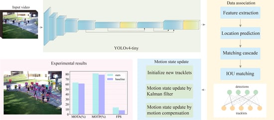
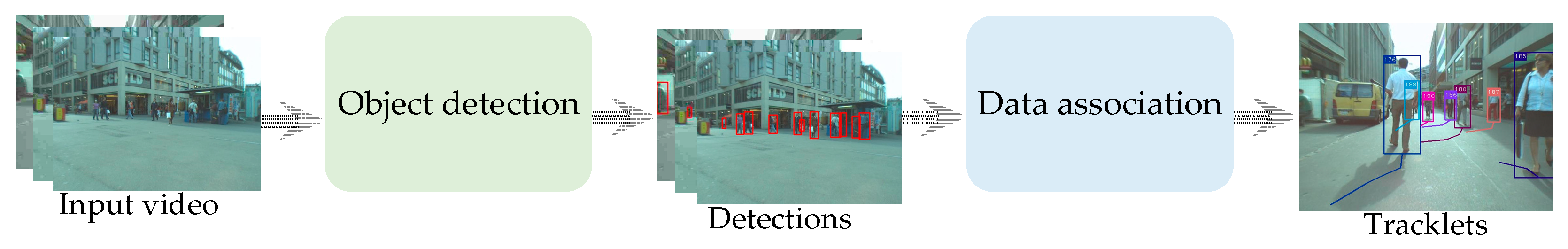
3.1. Overall Framework of SORT-YM

As shown in Figure 3, we demonstrate the overall framework of the SORT-YM based on the feature extraction, matching cascade, intersection-over-union (IOU) matching, motion state updating, and output tracklets. We perform the flowchart of SORT-YM as follows:

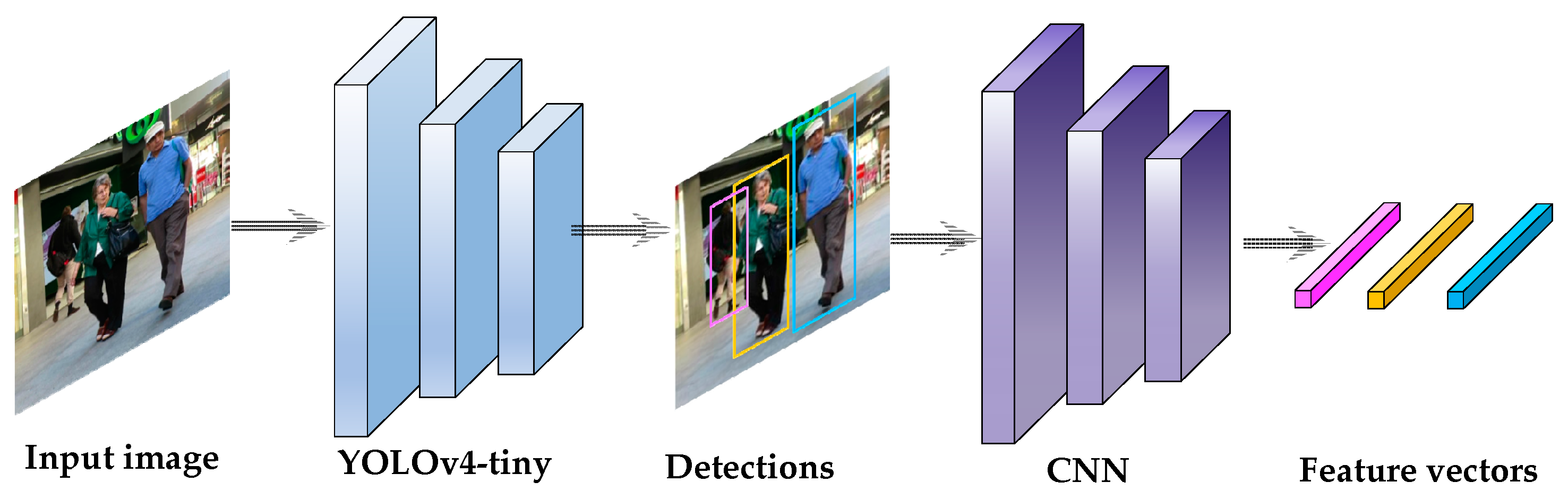
• Step 1. The detection generation: We apply efficient YOLOv4-tiny to produce the detections for each video frame.
• Step 2. The appearance feature extraction: The appearance features of each detection are extracted through a convolutional neural network.
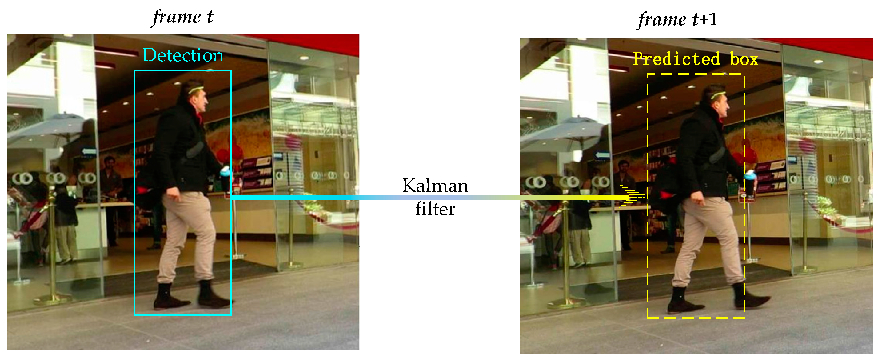
• Step 3. The tracklet location prediction: We can obtain the predicted location of every tracklet in the next frame by utilizing the Kalman filter.
• Step 4. The matching cascade: We calculate the appearance feature similarity and location distance between the confirmed tracklets and detections. After that, the association results of the confirmed tracklets and detections are obtained through the Hungarian algorithm.
• Step 5. The IOU matching: We compute the intersection-over-union (IOU) between the detection boxes and predicted bounding boxes of candidate tracklets. After that, the association results of the candidate tracklets and detections are obtained through the Hungarian algorithm.
• Step 6. The motion state updating: We update the motion state of the tracklets by the Kalman filter and the motion prediction model. Then, we initialize new tracklets for unassociated detections.

3.2. YOLOv4-Tiny Model

The performance of the tracking-by-detection paradigm can be heavily affected by the detections. The MOT system with a two-stage detector is limited in tracking speed. Moreover, the runtime increases significantly as the number of objects increases. Therefore, comprehensively considered the tracking performance and speed, we apply efficient YOLOv4-tiny to realize a trade-off between detection accuracy and speed. In contrast to Faster R-CNN [8], the YOLOv4-tiny is a lightweight convolutional network, which achieves 371 FPS on GTX 1080Ti. The network structure of the YOLOv4-tiny [28] is shown in Figure 4.

Different from Faster R-CNN, the YOLOv4-tiny employs the CSPDarknet53-tiny network as a backbone. The CSPDarknet53-tiny network applies CBLblock and CSPBlock for feature extraction. The CBLblock contains the convolution operation, batch normalization, and activation function. To further reduce computational overhead, the YOLOv4-tiny utilizes the LeakyRelu function as an activation function, which is defined by:

$$y_i=\{\begin{array}{c}{x}_i,x_i\ge 0\\ \frac{x_i}{a_i},x_i<0\end{array}$$

(1)

where a_i is a constant parameter larger than 1. By adopting a cross-stage partial connections structure, the CSPBlock divides the input feature map into two parts and concatenates the two parts in the cross-stage residual edge. Meanwhile, the CSPBlock can significantly reduce the computational complexity by 10–20% while ensuring the detection accuracy of the network. In the multi-feature fusion stage, the YOLOv4-tiny constructs a feature pyramid network to extract feature maps. Through the feature pyramid network, we can obtain two effective feature maps of different sizes. To estimate the detections, the YOLOv4-tiny adopts the fused feature maps by the classification and location of the targets.

In the process of prediction, the YOLOv4-tiny divides the input images into grids with the size S × S. For each grid, the network utilizes three anchors to predict objects. As a result, S × S × 3 bounding boxes will be generated for each input image. The anchors in the grids that contain the center of objects will be used to regress the detection boxes. Subsequently, to reduce redundant bounding boxes, we can calculate the confidence score of each detection box. The detections with a confidence score lower than the preset threshold will be removed. The confidence score of each detection is defined as:

$$Conf=Pr(object)\times Io{U}_{pred}^{truth},$$

(2)

where Pr(object) denotes the possibility that the detection box contains an object. Then, the $Io{U}_{pred}^{truth}$ represents the IOU between the predicted bounding box R^pred and the ground-truth box R^truth, which can be denoted as:

$$Io{U}_{pred}^{truth}=\frac{\left|R^{pred}\cap R^{truth}\right|}{\left|R^{pred}\cup R^{truth}\right|}.$$

(3)

Then, the YOLOv4-tiny applies the classification loss function to measure the category error between the predicted box and the ground-truth box. The classification loss function is:

$$L_{cls}=-{\displaystyle \sum _{i=0}^{S\times S}{I}_{ij}^{obj}{\displaystyle \sum _{c\in classes}\left[{\widehat{p}}_i(c)\log (p_i(c))+(1-{\widehat{p}}_i(c))\log (1-p_i(c))\right]}}.$$

(4)

Among them, if the j-th anchor in the i-th grid contains an object, $I_{ij}^{obj}$ = 1, otherwise $I_{ij}^{obj}$ = 0. The ${\widehat{p}}_i(c)$ and $p_i(c)$ are the real possibility and predicted the possibility of the target in the anchor that belongs to class c. After that, the YOLOv4-tiny employs the CIoU loss function for bounding box regression. The CIoU loss function is defined as:

$$L_{CIoU}=1-Io{U}_{pred}^{truth}+\frac{{\rho }^2(b^{pred},b^{truth})}{c^2}+\frac{16}{{\pi }^4}\frac{{\left(\arctan \frac{w^{truth}}{h^{truth}}-\arctan \frac{w^{pred}}{h^{pred}}\right)}^4}{1-Io{U}_{pred}^{truth}+\frac{4}{{\pi }^2}{\left(\arctan \frac{w^{truth}}{h^{truth}}-\arctan \frac{w^{pred}}{h^{pred}}\right)}^2},$$

(5)

where ${\rho }^2(\cdot )$ denotes the Euclidean distance. b^pred and b^truth represent the central points of R^pred and R^truth, respectively. c indicates the diagonal length of the smallest enclosing rectangle covering R^pred and R^truth. w and h signify the width and height of the bounding box, respectively. In Figure 5, we demonstrate detection results of the YOLOv4-tiny. After that, we send the detection results of each video frame to the data association model to receive the association results of targets.

3.3. Data Association

3.3.1. Feature Extraction

In order to improve the tracking accuracy and robustness in complex scenes, such as the interaction between targets and occlusion, we carry out the data association by extracting the target appearance information. By using a convolution neural network (CNN), we can pick up the appearance features of all detections in the current image. After counting the aspect ratio of the ground-truth bounding boxes of the MOT-16 training set [26], we found that approximately 70% of pedestrians have an aspect ratio between 0.3 and 0.7. Thus, the input detections are reshaped to 128 × 64 and presented to the CNN in RGB color space. As shown in

Table 1. The CNN architecture.

	Patch Size/Stride	Output Size
Conv 1	3 × 3/1	32 × 128 × 64
Conv 2	3 × 3/1	32 × 128 × 64
Max-pooling 3	3 × 3/2	32 × 64 × 32
Residual block 4	3 × 3/1	32 × 64 × 32
Residual block 5	3 × 3/1	32 × 64 × 32
Residual block 6	3 × 3/2	64 × 32 × 16
Residual block 7	3 × 3/1	64 × 32 × 16
Residual block 8	3 × 3/2	128 × 16 × 8
Residual block 9	3 × 3/1	128 × 16 × 8
Dense 10		128
Normalization		128

, the CNN structure applies two convolution layers, a max-pooling layer, and six residual blocks to squeeze the size of the feature map into 16 × 8. As a result, we can obtain the global feature vector of dimensionality 128 in a dense layer. Finally, the feature vector is normalized.

We use the cosine-margin-triplet loss function [29] to train the feature extractor. The cosine-margin-triplet is defined as:

$$L=-\frac{1}{N}{\displaystyle \sum _{i=1}^N\log }\frac{\exp (f^{\top }{f}^{+})}{\exp (f^{\top }{f}^{+})+\exp (f^{\top }{f}^{-})},$$

(6)

where N denotes the number of detections over a batch of video frames, $f^{\top }$ indicates the anchor of the triplet. $f^{+}$ and $f^{-}$ is the positive and negative sample with respect to $f^{\top }$, respectively. The function aims to minimize the distance between the positive pair and enlarge the distance between the negative pair. The dot product between the pair of feature vectors is defined as:

$$f^{\top }{f}^{+}=\Vert f^{\top }\Vert \Vert f^{+}\Vert \cos (\theta )$$

(7)

where $\Vert ·\Vert$ denotes the two-norm of the feature vector and $\theta$ indicates the angle between the two vectors. This network contains a total of 2,800,864 parameters. Therefore, it realizes a fast calculation speed that satisfies the real-time performance. We train the feature extraction network on the popular person re-identification dataset [30], which contains 1261 pedestrians and more than 1,100,000 video frames. The CNN is tested on the Nvidia RTX3070 GPU (NVIDIA, Santa Clara, CA, USA) and Nvidia GTX1050 GPU (NVIDIA, Santa Clara, CA, USA), and the results show that it only takes 0.85 ms and 0.93 ms on average to extract the feature of an object, respectively. Thus, this CNN is suitable for real-time tracking on different hardware devices. We send all detections to the trained CNN network, and the feature vectors of each target can be obtained as shown in Figure 6.

3.3.2. Motion State Estimation

In complex tracking scenarios, associating detections and tracklets based on appearance feature only produces a large number of ID switches. To further improve tracking accuracy, it is necessary to introduce the motion information of targets. As the velocity of targets in adjacent video frames is relatively stable, we apply the Kalman filter [31] to predict the motion state of targets in the next frame, as shown in Figure 7.

Firstly, we initialize a new motion state model based on the detection results for targets that first appear in the video. The motion state model is defined as:

$$x={[c_x,c_y,r,h,v_x,v_y,v_r,v_h]}^{\mathrm{T}},$$

(8)

where [c_x, c_y, r, h] is the location state of the target. Among them, (c_x, c_y) denotes the center coordinate of the target, and r and h denote the aspect ratio and height of the bounding box, respectively. [v_x, v_y, v_r, v_h] is the velocity state of targets, which indicates the target’s speed in four directions. Then, for each new target based on the height of the bounding box, we initialize the covariance matrix P₀ empirically, which is defined as:

$${\mathit{P}}_0=\left[\begin{array}{cccccccc}\frac{h^2}{100}& 0& 0& 0& 0& 0& 0& 0\\ 0& \frac{h^2}{100}& 0& 0& 0& 0& 0& 0\\ 0& 0& 10^{-4}& 0& 0& 0& 0& 0\\ 0& 0& 0& \frac{h^2}{100}& 0& 0& 0& 0\\ 0& 0& 0& 0& \frac{h^2}{256}& 0& 0& 0\\ 0& 0& 0& 0& 0& \frac{h^2}{256}& 0& 0\\ 0& 0& 0& 0& 0& 0& 0& 0\\ 0& 0& 0& 0& 0& 0& 0& \frac{h^2}{256}\end{array}\right],$$

(9)

According to the target motion state at frame k − 1, we estimate the motion state of the object in frame k by the Kalman filter as:

$${\widehat{\mathit{x}}}_k^{-}=\mathit{F}{\widehat{\mathit{x}}}_{k-1},$$

(10)

where ${\widehat{\mathit{x}}}_{k-1}$ denotes the motion state of the target in frame k − 1, and ${\widehat{\mathit{x}}}_k^{-}$ indicates the predicted motion state in frame k. F is the state-transition matrix, which is defined as:

$$\mathit{F}=\left[\begin{array}{cccccccc}1& 0& 0& 0& dt& 0& 0& 0\\ 0& 1& 0& 0& 0& dt& 0& 0\\ 0& 0& 1& 0& 0& 0& dt& 0\\ 0& 0& 0& 1& 0& 0& 0& dt\\ 0& 0& 0& 0& 1& 0& 0& 0\\ 0& 0& 0& 0& 0& 1& 0& 0\\ 0& 0& 0& 0& 0& 0& 1& 0\\ 0& 0& 0& 0& 0& 0& 0& 1\end{array}\right],$$

(11)

After that, by the covariance matrix ${\mathit{P}}_{k-1}$ in the previous frame, we can computer the covariance matrix at the current frame as:

$${\mathit{P}}_k^{-}=\mathit{F}{\mathit{P}}_{k-1}{\mathit{F}}^{\mathrm{T}}+\mathit{Q},$$

(12)

where Q and ${\mathit{P}}_k^{-}$ are the noise matrix and the predicted covariance matrix, respectively.

As shown in Figure 3, we divide the tracklets into confirmed tracklets and unconfirmed tracklets. The confirmed tracklets are formed by the associated detections of more than three frames. The other tracklets are denoted as unconfirmed tracklets. For the confirmed tracklets, we will associate them with subsequent detections by subsequent cascade matching. For unconfirmed tracklets and remaining unassociated tracklets, we will associate them with detections by subsequent IOU matching.

3.3.3. Matching Cascade

To improve the tracking accuracy and reduce the identity switches effectively, we comprehensively consider the appearance feature and motion state of objects. The matching cascade stage is performed as follows.

Firstly, we compute the cosine distance between the confirmed tracklet feature and the detection feature. We denote the i-th tracklet feature and the j-th detection feature as A = (a₁, a₂,…, a₁₂₈) and B = (b₁, b₂, …, b₁₂₈), respectively. The mathematical expression of cosine distance between tracklet feature and detection feature can be formulated as:

$$c_{i,j}=1-\frac{{\displaystyle \sum _{i=1}^{128}{a}_i{b}_i}}{\sqrt{{\displaystyle \sum _{i=1}^{128}{a}_i^2}}\sqrt{{\displaystyle \sum _{i=1}^{128}{b}_i^2}}},$$

(13)

The smaller $c_{i,j}$ is, the higher similarity between the confirmed tracklet and detection is.

Then, we construct all c_i,j into the cosine distance matrix C. Considering that the location of pedestrians changes little in the adjacent two frames, we get rid of the matching pairs whose Mahalanobis distance is too large. For the i-th confirmed tracklet, we calculate the squared Mahalanobis distance with the j-th detection as follows:

$$b_{i,j}={({\mathit{l}}_j-{\mathit{x}}_i)}^{\mathrm{T}}{\mathsf{\Sigma }}_i{}^{-1}({\mathit{l}}_j-{\mathit{x}}_i),$$

(14)

where x_i indicates the predicted location of the i-th confirmed tracklet, and l_j denotes the location of the j-th detection. ${\mathsf{\Sigma }}_i$ is the first four rows and four columns of the predicted covariance matrix ${\mathit{P}}_k^{-}$. The smaller $b_{i,j}$ is, the closer the confirmed tracklet and detection are.

If b_i,j is larger than the preset threshold ζ, we set the corresponding c_i,j of C to 10. Next, we utilize C as the input of the Hungarian algorithm [32] to obtain the association results through the matching cascade. The Hungarian algorithm is a commonly used approach for solving assignment problems. By means of this method, it can be obtained that the association results are both similar in appearance feature and location.

3.3.4. IOU Matching

There are still some unassociated tracklets and detections after the above matching method. We use the unassociated confirmed tracklets and unconfirmed tracklets as candidate tracklets. Then, we send all candidate tracklets and unassociated detections to participate in IOU matching.

In the process of IOU matching, we first compute the IOU between the predicted boxes of the candidate tracklets and unassociated detection boxes. Then, we construct the matrix U based on 1-IOU of each pair of tracklet and detection. The element u_i,j of U denotes the value of 1-IOU between the i-th candidate tracklet and the j-th detection. If u_i,j is smaller, it means that the overlap ratio of the two objects is larger, and the possibility of being the same target is greater. After that, we employ U as the input of the Hungarian algorithm to obtain the association results through the IOU matching.

3.3.5. Motion State Updating

The involves combining the association results of matching cascade and IOU matching, and dividing all tracklets into associated tracklets and unassociated tracklets. In addition, all detections are divided into matched detections and unmatched detections. Then, we update the estimated motion states for tracklets and initialize new tracklets for unmatched detections.

For associated tracklets, the estimated motion states are updated by means of a Kalman filter. Firstly, the tractor computes Kalman gain. Determining Kalman gain is a critical step in establishing the Kalman filter model, which significantly impacts the efficiency and accuracy of filtering. Kalman gain can be calculated as follows:

$${\mathit{K}}_k=\frac{{\mathit{P}}_k^{-}{\mathit{H}}^{\mathrm{T}}}{\mathit{H}{\mathit{P}}_k^{-}{\mathit{H}}^{\mathrm{T}}+\mathit{R}},$$

(15)

where H denotes the transition matrix from state quantity to observation, and R indicates the observation noise covariance matrix. Then, updating the estimated motion state of the tracklets by the matched detections as follows:

$${\widehat{\mathit{x}}}_k={\widehat{\mathit{x}}}_k^{-}+{\mathit{K}}_k({\mathit{z}}_k-\mathit{H}{\widehat{\mathit{x}}}_k^{-}),$$

(16)

where ${\widehat{\mathit{x}}}_k$ denotes the modified motion state for the tracklets, and z_k indicates the location vector of the matched detections.

Finally, updating the covariance matrix for tracklets is as follows:

$${\mathit{P}}_k=(\mathit{I}-{\mathit{K}}_k\mathit{H}){\mathit{P}}_k^{-},$$

(17)

where P_k denotes the modified covariance matrix for tracklets, and I is an identity matrix.

As for unmatched detections, we regard them as new objects in the video and initialize new motion states for them using Equation (8).

3.3.6. Motion Prediction Strategy

If the motion states of the unassociated tracklets are not updated, the difficulty of re-associating the object with subsequent detections increases significantly after a period of disappearance. When the object appears in the video again, it is very likely to increase the identity switches. Therefore, we design a motion prediction strategy to estimate the moving speed in four directions of the occluded objects. Since the occluded objects may be legible in the previous frames, we utilize the location of the objects in the earlier frames to estimate the speed of the objects, thereby predicting the possible location of the occluded objects.

Firstly, the motion prediction model gets the velocity state model [v_x, v_y, v_r, v_h] of the unassociated tracklets in previous frames. As different video frames are of different importance for predicting the current location, we give weights to each frame’s velocity state model based on the time interval. The velocity state model closer to the current time has a higher weight. The weight for each frame can be calculated as:

$$w_i=\frac{i-n}{{\displaystyle \sum _{\delta =1}^{m-n+1}\delta }},s.t.n\le i\le m$$

(18)

where n represents the frame index when the object enters the video for the first time, and m indicates the current frame index. Subsequently, we subtract the speed of the object in the past two adjacent frames to get the acceleration of the object in each frame in the past. After that, we sum up the weighted acceleration of the object in each frame in the earlier frames to obtain the predicted acceleration. The predicted acceleration of the object can be calculated as:

$${\mathit{a}}_{pred}={\displaystyle \sum _{i=n}^{m-1}{w}_i\cdot (v_{i+1}-v_i)}.$$

(19)

Then, based on the weight of each object in previous frames, we weighted sum the speed of the object in the past. After that, we sum the result of the weighted summation to the predicted acceleration to obtain the predicted velocity in the current frame as follows:

$${\mathit{v}}_{pred}={\mathit{a}}_{pred}+{\displaystyle \sum _{i=n}^{w-1}{w}_i\cdot {\mathit{v}}_i}.$$

(20)

Finally, we add the estimated velocity to the location in the previous frame locat_k−1 to obtain the predicted location locat_pred of the object in the current frame as follows:

$$\mathit{l}\mathit{o}\mathit{c}\mathit{a}{\mathit{t}}_{pred}=\mathit{l}\mathit{o}\mathit{c}\mathit{a}{\mathit{t}}_{k-1}+{\mathit{v}}_{pred}$$

(21)

The main steps of the SORT-YM are shown in Algorithm 1.

Algorithm 1 SORT-YM
Input: A video with T frames
Output: Tracklets of the video
fort = 1,…, T do
	Detect the location $D_k^t$ of objects by YOLOv4-tiny
	Extract the appearance feature $F_k^t$ of each detected object through the CNN
	Predict new location ${\widehat{x}}_k^{-}$ of each tracklet using Kalman filter
	foreach confirmed trackletdo
		Calculate the cost matrix C = [ci,j] using cosine distance between the feature of tracklet and each detection
		Calculate the Mahalanobis distance matrix B = [bi,j] between the predicted location of the i-th tracklet and the j-th detection
		ifbi,j ≥ ζ do
		ci,j = 10
		end
	end
	Obtain the association results of matching cascade using Hungarian algorithm based on C
	foreach unconfirmed tracklet and unassociated confirmed trackletdo
		Calculate the IOU matrix U = [ui,j] using the IOU between the predicted box of tracklet and each detection box
	end
	Obtain the association results of IOU matching using Hungarian algorithm based on U
	Integrate the association results of matching cascade and IOU matching
	foreach associated trackletdo
		Update the predicted location using Kalman filter
	end
	foreach unassociated trackletdo
		ifthe tracklet is continuously unassociated for 30 framesdo
		Remove the tracklet from candidates
		else
		Predict the location using motion prediction
		end
	end
	fordetections not associated with trackletsdo
		Initialize a new tracklet based on the detection results
	end
end

4. Experimental Results and Analyses

In this section, we first describe the details of our experiments. Then, we evaluate the performance of the proposed algorithm on two datasets. Meanwhile, we compare the performance of the algorithm with state-of-the-art methods.

4.1. Experimental Settings

The Mahalanobis distance threshold ζ is set to 9.5. Based on the prior conditions of pedestrians, we design the anchor boxes in the light of numbers and aspect ratios. We set all anchor boxes to an aspect ratio of 1:3. Meanwhile, we utilize three anchors for each scale. The height of the anchors ranges from 24 to 640. At the same time, we construct an enormous dataset by integrating training images and annotations from 7 datasets for pedestrian detection, including the ETH dataset [33], CityPersons dataset [34], CalTech dataset [35], CUHK-SYSU dataset [36], PRW dataset [37], MOT-15 dataset [23], and MOT-16 dataset [26], to improve the tracking performance of the proposed algorithm. Additionally, our experiment is developed based on TensorFlow 2.3 using Python 3.8 and PyCharm 2020.3. Additionally, our experiment equipment is a PC with an i5-10600KF CPU (Intel, Santa Clara, CA, USA) and an Nvidia RTX3070 GPU (NVIDIA, Santa Clara, CA, USA). We train the network with standard stochastic gradient descent for 30 epochs. The learning rate of the network is initially set as 10⁻², and it decays to 10⁻³ at the 25th epoch.

4.2. Dataset and Evaluation Metrics

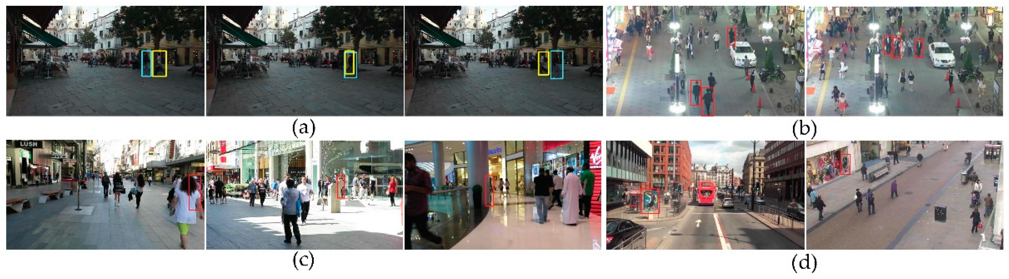
4.2.1. Dataset Protocol

We evaluate the performance of our algorithm on the testing sets of two extensively used MOT benchmarks: MOT-15 and MOT-16. The MOT-15 dataset contains 22 video sequences, including 11 training sets and 11 testing sets, with over 11,000 video frames in total. The main difficulties of MOT-15 are as follows:

• A large number of objects: The number of the annotated bounding boxes for all testing video sequences is 61,440. Therefore, it is difficult for the algorithm to achieve a high tracking accuracy with a fast speed.
• Static or moving camera: Among the 11 testing video sequences, six videos are taken by a static camera, and a moving camera takes the remaining videos. These two modes of videos increase the requirement for the algorithm to predict the location of tracklets.

The MOT-16 contains seven testing video sequences in total. Compared to the MOT-15, the MOT-16 is a more challenging dataset. The scenarios of the videos in MOT-16 are more crowded and more complex. In addition to the challenges of the MOT-15, there still exists the following challenges in MOT-16 video sequences:

• Different viewpoints: Each video sequence has a different viewpoint owing to the different heights of the camera. Videos from multiple perspectives increase the difficulty of object detection and feature extraction.
• Varying weather conditions: A sunny weather video may contain some shadows, while the videos with dark or cloudy weather have lower visibility, making pedestrian detection and tracking more difficult.

4.2.2. Evaluation Metrics

To evaluate the tracking performance, we utilize the evaluation metrics provided by MOT Challenge Benchmark [38]. First, we adopt the multi-object tracking accuracy (MOTA) to evaluate the robustness of our algorithm. MOTA comprehensively considers three types of tracking errors, and it is defined as:

$$\mathrm{MOTA}=1-\frac{{\displaystyle {\sum }_t\left(\mathrm{F}{\mathrm{N}}_t+\mathrm{F}{\mathrm{P}}_t+\mathrm{I}\mathrm{D}{\mathrm{s}}_t\right)}}{{\displaystyle {\sum }_t\mathrm{G}{\mathrm{T}}_t}},$$

(22)

where t is the index of the video frame, and FN denotes the number of false negatives, representing the ground-truth objects that are not detected by the algorithm. GT is the number of ground-truth objects in all video sequences. IDs indicates the number of ID switches for all objects. Then, the tracking precision of the method is evaluated through the multiple object tracking precision (MOTP), which is defined as:

$$\mathrm{MOTP}=\frac{{\displaystyle {\sum }_{t,i}{d}_{t,i}}}{{\displaystyle {\sum }_t{c}_t}},$$

(23)

where $c_t$ represents the number of the objects tracked correctly in frame t. $d_{t,i}$ indicates the bounding box overlap of the i-th successfully tracked object with the ground-truth object in frame t. Mostly tracked objects (MT) is the ratio of tracklets that are tracked to more than 80%. Mostly lost objects (ML) is the ratio of tracklets that are tracked for less than 20%. After that, fragmentations (FM) indicates the number of interruptions for all ground-truth tracklets. Finally, we evaluate the speed of the algorithm through the frames per second (FPS).

4.3. Comparison with the State-of-the-Art Algorithms

4.3.1. Experiment on MOT-15 Dataset

We test the performance of the SORT-YM on the MOT-15 dataset. We demonstrate the comparative quantitative results on the MOT-15 dataset, as shown in

Table 2. The quantitative results by our proposed method and state-of-the-arts on MOT-15 dataset. ↑ denotes that higher is better and ↓ represents the opposite. The best and sub-optimal results are highlighted in bold and italics.

Method	Mode	MOTA↑	MOTP↑	MT↑	ML↓	IDs↓	FN↓	FM↓	FPS↑
SiameseCNN [39]	Offline	29.0%	71.2%	8.5%	48.4%	639	37,798	1316	52.8
Quad-CNN [40]	Offline	33.8%	73.4%	12.9%	36.9%	703	32,061	1430	3.7
RMNet [41]	Offline	28.1%	74.3%	-	-	477	36,952	790	16.9
MHT-DAM [17]	Online	32.4%	71.8%	16.0%	43.8%	435	32,060	826	0.7
RNN_LSTM [42]	Online	19.0%	71.0%	5.5%	45.6%	1490	36,706	2081	165.2
STAM [43]	Online	34.3%	70.5%	11.4%	43.4%	348	34,848	1463	0.5
HybridDAT [44]	Online	35.0%	72.6%	11.4%	42.2%	358	31,140	1267	4.6
AMIR [45]	Online	37.6%	71.7%	15.8%	26.8%	1026	29,397	2024	1.0
AP_RCNN [46]	Online	38.5%	72.6%	8.7%	37.4%	586	33,204	1263	6.7
RAN_DPM [47]	Online	35.1%	70.9%	13.0%	42.3%	381	32,717	1523	5.4
TripT + BF [48]	Online	37.1%	72.5%	12.6%	39.7%	580	29,732	1193	1.0
SORT [49]	Online	33.4%	72.1%	11.7%	30.9%	1001	32,615	1764	260.0
MNC + CPM [50]	Online	32.1%	70.9%	13.2%	30.1%	1687	33,473	2471	-
AP_RCNN [46]	Online	53.0%	75.5%	29.1%	20.2%	708	22,984	1476	6.7
RAN_FRCNN [47]	Online	56.5%	73.0%	45.1%	14.6%	428	16,921	1364	5.1
SORT-YM (proposed)	Online	58.2%	79.3%	44.4%	12.2%	604	20,753	901	24.4

. We compared SORT-YM with 3 offline approaches and 13 online approaches. SORT-YM achieves state-of-the-art performance in terms of MOTA (58.2%), MOTP (79.3%), and ML (12.2%). Meanwhile, SORT-YM ranks second on MT (44.4%) and FN (20753). In addition, the tracking speed of our proposed method is faster than most online approaches. The tracking speed of SiameseCNN, RNN_LSTM, and SORT is faster than SORT-YM. However, SORT-YM has an obvious advantage in tracking accuracy.

The visual tracking result on the MOT-15 dataset of SORT-YM is shown in Figure 8. As shown in Figure 8b–d,g, SORT-YM obtain accurate tracklets in videos taken by a moving camera. Among them, our proposed method maintains robust tracking performance in Figure 8c with large shadows and small objects. As shown in Figure 8a,e,f, SORT-YM achieves higher tracking accuracy in videos taken by a static camera. Among them, tracking bounding box drift does not occur in complex scenes with interference with many similar objects, as shown in Figure 8e. In addition, our algorithm keeps strong robustness in crowded tracking scenarios with many occlusions and interactions between objects, as shown in Figure 8f. In summary, SORT-YM shows high tracking accuracy and outputs relatively complete tracklets on the MOT-15 dataset.

4.3.2. Experimental on MOT-16 Dataset

We first perform ablation analysis on the MOT-16 dataset to verify the necessity of each component in SORT-YM. We apply the Deep SORT [24] as our baseline, and we remove proposed components to investigate the contribution to our method. The comparison results are shown in

Table 3. The ablation experiments on the MOT-16 dataset.

Methods	MOTA↑	MOTP↑	ML↓	IDs↓	FN↓	FM↓	FPS↑
Baseline	61.4%	79.1%	18.2%	781	56,668	2008	14
Baseline + YOLOv4-tiny	62.6%	81.2%	17.3%	739	30,771	1995	23.8
Baseline + motion prediction	62.3%	79.6%	17.0%	746	28,768	1923	13.7
SORT-YM	63.4%	81.4%	16.7%	707	21,439	1888	23.1

.

Effect of YOLOv4-tiny. To evaluate the effectiveness of using YOLO-tiny, we perform an experiment to see the benefit. As shown in Table 3, compared to the Deep SORT baseline, which utilizes the Faster R-CNN [8] as the detector, the tracking speed of the algorithm with YOLOv4-tiny significantly improves. Meanwhile, the MOTA and MOTP increase by 1.2% and 0.9%, respectively.

Effect of motion prediction. We also experiment to verify the necessity of motion prediction. We added the motion prediction module to the Deep SORT baseline. The experimental results show that adding the motion prediction module reduces the number of FN and FM by 27900 and 85, respectively. In addition, compared with the case where no motion prediction is employed, SORT-YM improves the MOTA by 0.8%. Meanwhile, the number of FN and FM is reduced by 9332 and 107, respectively, due to the strong ability of the motion prediction to retrieve the lost objects.

To further measure the tracking performance, we compare the SORT-YM with another 14 recent tracking methods on the MOT-16 dataset, including MHT_DAM [17], Deep SORT [24], SORT [49], TBD [51], LTTSC-CRF [52], LINF [53], JMC [54], NOMTwSDP16 [55], NOMT [55], KDNT [56], LMP_P [57], OVBT [58], EAMTT_private [59], and EAMTT_public [59].

As shown in

Table 4. The quantitative results by our proposed method and state-of-the-arts on MOT-16 dataset. ↑ Denotes that higher is better and ↓ represents the opposite. The best and sub-optimal results are highlighted in bold and italics.

Method	Mode	MOTA↑	MOTP↑	MT↑	ML↓	IDs↓	FN↓	FM↓	FPS↑
TBD	Offline	33.7%	76.5%	7.2%	54.2%	2418	112,587	2252	-
LTTSC-CRF	Offline	37.6%	75.9%	9.6%	55.2%	481	101,343	1012	0.6
LINF	Offline	41.0%	74.8%	11.6%	51.3%	430	99,224	963	4.2
MHT_DAM	Offline	42.9%	76.6%	13.6%	46.9%	499	97,919	659	0.8
JMC	Offline	46.3%	75.7%	15.5%	39.7%	657	90,914	1114	0.8
NOMT	Offline	46.4%	76.6%	18.3%	41.4%	359	87,565	504	2.6
NOMTwSDP16	Offline	62.2%	79.6%	32.5%	31.1%	406	-	642	3
KDNT	Offline	68.2%	79.4%	41.0%	19.0%	933	45,605	1093	0.7
LMP_P	Offline	71.0%	80.2%	46.9%	21.9%	434	44,564	587	0.5
OVBT	Online	38.4%	75.4%	7.5%	47.3%	1321	99,463	2140	0.3
EAMTT_public	Online	38.8%	75.1%	7.9%	49.1%	965	102,452	1657	11.8
EAMTT_private	Online	52.5%	78.8%	19.0%	34.9%	910	81,223	1321	12
SORT	Online	59.8%	79.6%	25.4%	22.7%	1423	63,245	1835	60
Deep SORT (baseline)	Online	61.4%	79.1%	32.8%	18.2%	781	56,668	2008	14
SORT-YM	Online	63.4%	81.7%	33.8%	16.7%	707	21,439	1888	23.1

, SORT-YM achieves state-of-the-art performance in terms of MOTP (81.7%), ML (16.7%), and FN (21439). Meanwhile, our proposed method reaches the highest MOTA (63.4%) in online methods. Compared to KDNT and LMP_P, the speed of SORT-YM is much faster. In fact, SORT-YM achieves the second-fastest tracking speed. Compared with the Deep SORT baseline, the SORT-YM has improved in all indexes. Among them, MOTA and MOTP increase by 2% and 2.6%, respectively, which shows that our algorithm has improved both in tracking accuracy and precision. In addition, SORT-YM reduces 74 ID switches, which indicates that our algorithm can better deal with the interference of occlusion and interaction. Meanwhile, the tracking speed of SORT-YM increases significantly. In general, SORT-YM achieved high performance on both tracking robustness and speed on the MOT-16 dataset.

The visual tracking result on the MOT-16 dataset of SORT-YM is shown in Figure 9. In the dark tracking scenario shown in Figure 9a, SORT-YM achieves strong robustness. Meanwhile, our algorithm achieves high tracking accuracy for both dark and bright objects, as shown in Figure 9d. In the crowded scene with a large number of occlusions shown in Figure 9b, since the proposed motion prediction strategy can predict the location of the occluded objects, SORT-YM still accurately obtain the relatively complete tracklets of most objects. In addition, our proposed method shows strong tracking robustness for objects of different sizes, as shown in Figure 9c,e. In conclusion, SORT-YM shows high tracking accuracy and outputs relatively complete tracklets in various complex scenes of the MOT-16 dataset.

5. Conclusions

Focusing on the problem that it is difficult to predict the location of occluded objects in existing multi-object tracking methods, this study designs a motion prediction strategy for predicting the location of the lost objects. Since the occluded objects may be legible in the earlier frames, we use the information from multiple frames in the past to predict the location of the occluded objects. To further improve the tracking performance of the algorithm, we utilize YOLOv4-tiny as our detector. Experimental results on the MOT-15 dataset and MOT-16 dataset show that the SORT-YM achieves state-of-the-art results on multiple indicators and improves the tracking speed. Comprehensively considering the tracking robustness and speed, SORT-YM is a competitive algorithm. Compared with the Deep SORT, our algorithm has a significant improvement in tracking performance. The future research focus is mainly on two aspects. One is improving the efficiency of the object detection algorithm and the feature extraction network to reach real-time tracking. Another is improving the Kalman filter to enhance the tracking robustness in complex scenarios.

References

1. He, Y.H.; Wei, X.; Hong, X.P.; Shi, W.W.; Gong, Y.H. Multi-Target Multi-Camera Tracking by Tracklet-to-Target Assignment. IEEE Trans. Image Process. 2020, 29, 5191–5205. [Google Scholar] [CrossRef]
2. Sun, S.J.; Akhtar, N.; Song, H.S.; Mian, A.S.; Shah, M. Deep Affinity Network for Multiple Object Tracking. IEEE Trans. Pattern Anal. Mach. Intell. 2021, 43, 104–119. [Google Scholar] [CrossRef] [Green Version]
3. Girshick, R.; Donahue, J.; Darrell, T.; Malik, J. Rich feature hierarchies for accurate object detection and semantic segmentation. In Proceedings of the IEEE Conference on Computer Vision and Pattern Recognition, Columbus, OH, USA, 23–28 June 2014; pp. 580–587. [Google Scholar]
4. Felzenszwalb, P.; Girshick, R.; McAllester, D.; Ramanan, D. Object detection with discriminative trained part-based models. IEEE Trans. Pattern Anal. Mach. Intell. 2009, 32, 1627–1645. [Google Scholar] [CrossRef] [PubMed] [Green Version]
5. Everingham, M.; Van, G.L.; Williams, C.; Winn, J.; Zisserman, A. The pascal visual object classes (VoC) challenge. Int. J. Comput. Vis. 2010, 88, 303–338. [Google Scholar] [CrossRef] [Green Version]
6. He, K.; Zhang, X.; Ren, S.; Sun, J. Spatial pyramid pooling in deep convolution networks for visual recognition. IEEE Trans. Pattern Anal. Mach. Intell. 2015, 37, 1904–1916. [Google Scholar] [CrossRef] [PubMed] [Green Version]
7. Girshick, R. Fast R-CNN. In Proceedings of the IEEE International Conference on Computer Vision, Santiago, Chile, 11–18 December 2015; pp. 1440–1448. [Google Scholar]
8. Ren, S.; He, K.; Sun, J. Faster R-CNN: Towards real-time object detection with region proposal networks. In Proceedings of the Neural Information Processing Systems, Montreal, QC, Canada, 7–12 December 2015; pp. 91–99. [Google Scholar]
9. Renmon, J.; Divvala, S.; Girshick, R.; Farhadi, A. You Only Look Once: Unified, Real-Time Object Detection. In Proceedings of the IEEE Conference on Computer Vision and Pattern Recognition, Las Vegas, WA, USA, 27–30 June 2016; pp. 779–788. [Google Scholar]
10. Liu, W.; Anguelov, D.; Erhan, D.; Szegedy, C.; Reed, S.; Fu, C.Y.; Berg, A.C. SSD: Single shot multibox detector. In Proceedings of the European Conference on Computer Vision, Amsterdam, The Netherlands, 11–14 October 2016; pp. 21–37. [Google Scholar]
11. Renmon, J.; Farhadi, A. YOLO9000: Better, faster, stronger. In Proceedings of the IEEE Conference on Computer Vision and Pattern Recognition, Honolulu, HI, USA, 21–26 July 2017; pp. 6517–6525. [Google Scholar]
12. Lin, T.Y.; Goyal, P.; Girshick, R.; He, K.; Dollar, P. Focal loss for dense object detection. IEEE Trans. Pattern Anal. Mach. Intell. 2020, 42, 318–327. [Google Scholar] [CrossRef] [PubMed] [Green Version]
13. Lin, T.Y.; Maire, M.; Belongie, S.; Hays, J.; Perona, P.; Ramanan, D.; Dollar, P.; Zitnick, C.L. Microsoft coco: Common objects in context. In Proceedings of the European Conference on Computer Vision, Zurich, Switzerland, 6–12 September 2014; pp. 740–755. [Google Scholar]
14. Redmon, J.; Farhadi, A. Yolov3: An incremental improvement. arXiv 2018, arXiv:1804.02767. [Google Scholar]
15. Reid, D. An algorithm for tracking multiple targets. IEEE Trans. Automat. Contr. 1979, 24, 843–854. [Google Scholar] [CrossRef]
16. Krizhevsky, A.; Sutskever, I.; Hinton, G.E. Imagent classification with deep convolutional neural networks. Adv. Neural Inf. Process. Syst. 2012, 2, 1097–1105. [Google Scholar]
17. Kim, C.; Li, F.; Ciptadi, A.; Rehg, J.M. Multiple hypothesis tracking revisited. In Proceedings of the IEEE International Conference on Computer Vision, Santiago, Chile, 11–18 December 2015; pp. 4696–4704. [Google Scholar]
18. Fortmann, T.; Bar-Shalom, Y.; Scheffe, M. Sonar tracking of multiple targets using joint probabilistic data association. IEEE J. Oceanic Eng. 1983, 8, 173–184. [Google Scholar] [CrossRef] [Green Version]
19. Rezatofighi, S.H.; Milan, A.; Zhang, Z.; Shi, Q.F.; Dick, A.; Reid, I. Joint Probabilistic Data Association Revisited. In Proceedings of the IEEE International Conference on Computer Vision, Santiago, Chile, 11–18 December 2015; pp. 3047–3055. [Google Scholar]
20. Han, X.W.; Wang, Y.W.; Xie, Y.H.; Gao, Y.; Lu, Z. Multi-channel scale adaptive target tracking based on double correlation filter. Chin. J. Sci. Instrum. 2019, 40, 73–81. [Google Scholar]
21. Bae, S.H.; Yoon, K.J. Robust online multi-object tracking based on tracklet confidence and online discriminative appearance learning. In Proceedings of the IEEE Conference on Computer Vision and Pattern Recognition, Columbus, OH, USA, 23–28 June 2014; pp. 1218–1225. [Google Scholar]
22. Xiang, Y.; Alahi, A.; Savarese, S. Learning to track: Online multi-object tracking by decision making. In Proceedings of the IEEE Conference on Computer Vision and Pattern Recognition, Santiago, Chile, 11–18 December 2015; pp. 4705–4713. [Google Scholar]
23. Leal-Taixe, L.; Milan, A.; Reid, I.; Roth, S.; Schindler, K. MOTChallenge 2015: Towards a Benchmark for Multi-Target Tracking. arXiv 2015, arXiv:1504-01942. [Google Scholar]
24. Wojke, N.; Bewley, A.; Paulus, D. Simple online and realtime tracking with a deep association metric. In Proceedings of the IEEE International Conference on Image Processing, Beijing, China, 17–20 September 2017; pp. 3645–3649. [Google Scholar]
25. Chen, L.; Ai, H.Z.; Zhuang, Z.J.; Shang, C. Real-time Multiple People Tracking with Deeply Learned Candidate Selection and Person Re-Identification. In Proceedings of the IEEE Conference on Multimedia and Expo, San Diego, CA, USA, 23–27 July 2018; pp. 1–6. [Google Scholar]
26. Milan, A.; Leal-Taixe, L.; Reid, I.; Roth, S.; Schindler, K. Mot16: A benchmark for multi-object tracking. arXiv 2016, arXiv:1603.00831. [Google Scholar]
27. Wang, Z.; Zheng, L.; Liu, Y.X.; Wang, S.J. Towards real-time multi-object tracking. In Proceedings of the European Conference on Computer Vision, Glasgow, UK, 23–28 August 2020; pp. 107–122. [Google Scholar]
28. Bochkovskiy, A.; Wang, C.Y.; Liao, H.Y.M. YOLOv4: Optimal speed and accuracy of object detection. arXiv 2020, arXiv:2004.10934. [Google Scholar]
29. Unde, A.S.; Rameshan, R.M. MOTS R-CNN: Cosine-margin-triplet loss for multi-object tracking. arXiv 2021, arXiv:2102.03512. [Google Scholar]
30. Zheng, L.; Bie, Z.; Sun, Y.F.; Wang, J.D.; Su, C.; Wang, S.J.; Tian, Q. MARS: A Video Benchmark for Large-Scale Person Re-Identification. In Proceedings of the European Conference on Computer Vision, Amsterdam, The Netherlands, 8–16 October 2016; pp. 868–884. [Google Scholar]
31. Kalman, R. A New Approach to Linear Filtering and Prediction Problems. J. Basic Eng. 1960, 82, 35–45. [Google Scholar] [CrossRef] [Green Version]
32. Kuhn, H.W. The Hungarian Method for the assignment problem. Nav. Res. Logist. 2005, 52, 7–21. [Google Scholar] [CrossRef] [Green Version]
33. Ess, A.; Leibe, B.; Schindler, K.; Van, G.L. A mobile vision system for robust multi-person tracking. In Proceedings of the IEEE Conference on Computer Vision and Pattern Recognition, Anchorage, AK, USA, 23–28 June 2008; pp. 1857–1864. [Google Scholar]
34. Zhang, S.S.; Benenson, R.; Schiele, B. CityPersons: A Diverse Dataset for Pedestrian Detection. In Proceedings of the IEEE Conference on Computer Vision and Pattern Recognition, Honolulu, HI, USA, 21–26 July 2017; pp. 4457–4465. [Google Scholar]
35. Dollar, P.; Wojek, C.; Schiele, B.; Perona, P. Pedestrian detection: A benchmark. In Proceedings of the IEEE Conference on Computer Vision and Pattern Recognition, Miami, FL, USA, 20–25 June 2009; pp. 304–311. [Google Scholar]
36. Xiao, T.; Li, S.; Wang, B.C.; Lin, L.; Wang, X.G. Joint Detection and Identification Feature Learning for Person Search. In Proceedings of the IEEE Conference on Computer Vision and Pattern Recognition, Honolulu, HI, USA, 21–26 July 2017; pp. 3376–3385. [Google Scholar]
37. Zheng, L.; Zhang, H.H.; Sun, S.Y.; Chandraker, M.; Yang, Y.; Tian, Q. Person Re-identification in the Wild. In Proceedings of the IEEE Conference on Computer Vision and Pattern Recognition, Honolulu, HI, USA, 21–26 July 2017; pp. 3346–3355. [Google Scholar]
38. Dendofer, P.; Osep, A.; Milan, A.; Schindler, K.; Cremers, D.; Reid, I.; Roth, S.; Leal-Taixe, L. MOTChallenge: A Benchmark for Single-Camera Multiple Target Tracking. Int. J. Comput. Vis. 2020, 129, 845–881. [Google Scholar] [CrossRef]
39. Laura, L.T.; Cristian, C.F.; Konrad, S. Learning by tracking: Siamese cnn for robust target association. In Proceedings of the IEEE Conference on Computer Vision and Pattern Recognition, Las Vegas, NV, USA, 26 June–1 July 2016; pp. 418–425. [Google Scholar]
40. Son, J.; Beak, M.; Cho, M.; Han, B. Multi-Object Tracking with Quadruplet Convolutional Neural Networks. In Proceedings of the IEEE Conference on Computer Vision and Pattern Recognition, Honolulu, HI, USA, 21–26 July 2017; pp. 3786–3795. [Google Scholar]
41. Chen, L.T.; Peng, X.J.; Ren, M.W. Recurrent Metric Networks and Batch Multiple Hypothesis for Multi-Object Tracking. IEEE Access 2019, 7, 3093–3105. [Google Scholar] [CrossRef]
42. Milan, A.; Rezatofighi, S.H.; Dick, A.; Reid, I.; Schindler, K. Online Multi-Target Tracking Using Recurrent Neural Networks. In Proceedings of the AAAI Conference on Artificial Intelligence, San Francisco, CA, USA, 4–9 February 2017; pp. 4225–4232. [Google Scholar]
43. Chu, Q.; Ouyang, W.L.; Li, H.S.; Wang, X.G.; Liu, B.; Yu, N.H. Online Multi-Object Tracking Using CNN-based Single Object Tracker with Spatial-Temporal Attention Mechanism. In Proceedings of the IEEE International Conference on Computer Vision, Venice, Italy, 22–29 October 2017; pp. 4846–4855. [Google Scholar]
44. Yang, M.; Wu, Y.W.; Jia, Y.D. A Hybrid Data Association Framework for Robust Online Multi-Object Tracking. IEEE Trans. Image Process. 2017, 26, 5667–5679. [Google Scholar] [CrossRef] [Green Version]
45. Sadeghian, A.; Alahi, A.; Savarese, S. Tracking The Untrackable: Learning to Track Multiple Cues with Long-Term Dependencies. In Proceedings of the IEEE Conference on Computer Vision and Pattern Recognition, Honolulu, HI, USA, 21–26 July 2017; pp. 300–311. [Google Scholar]
46. Chen, L.; Ai, H.Z.; Shang, C.; Zhuang, Z.J.; Bai, B. Online multi-object tracking with convolutional neural networks. In Proceedings of the International Conference on Image Processing, Beijing, China, 17–20 September 2017; pp. 645–649. [Google Scholar]
47. Fang, K.; Xiang, Y.; Li, X.C.; Savarese, S. Recurrent Autoregressive Networks for Online Multi-Object Tracking. In Proceedings of the IEEE Winter Conference on Applications of Computer Vision, Lake Tahoe, NV, USA, 12–15 March 2018; pp. 466–475. [Google Scholar]
48. Xiang, J.; Zhang, G.S.; Hou, J.H. Online Multi-Object Tracking Based on Feature Representation and Bayesian Filtering Within a Deep Learning Architecture. IEEE Access 2019, 7, 27923–27935. [Google Scholar] [CrossRef]
49. Bewley, A.; Ge, Z.Y.; Ott, L.; Ramov, F.; Upcroft, B. Simple online and realtime tracking. In Proceedings of the IEEE International Conference on Image Processing, Phoenix, AZ, USA, 25–28 September 2016; pp. 3464–3468. [Google Scholar]
50. Bullinger, S.; Bodensteiner, C.; Arens, M. Instance flow based online multiple object tracking. In Proceedings of the IEEE International Conference on Image Processing, Beijing, China, 17–20 September 2017; pp. 785–789. [Google Scholar]
51. Geiger, A.; Lauer, M.; Wojek, C.; Stiller, C.; Urtasun, R. 3D traffic scene understanding from movable platforms. IEEE Trans. Pattern Anal. Mach. Intell. 2014, 36, 1012–1025. [Google Scholar] [CrossRef] [PubMed] [Green Version]
52. Le, N.; Heili, A.; Odobez, J.M. Long-term time-sensitive costs for crf-based tracking by detection. In Proceedings of the European Conference on Computer Vision, Amsterdam, The Netherlands, 8–16 October 2016; pp. 43–51. [Google Scholar]
53. Fagot-Bouquet, L.; Audigier, R.; Dhome, Y.; Lerasle, F. Improving multi-frame data association with sparse representations for robust near-online multi-object tracking. In Proceedings of the European Conference on Computer Vision, Amsterdam, The Netherlands, 8–16 October 2016; pp. 774–790. [Google Scholar]
54. Keuper, M.; Tang, S.; Zhongjie, Y.; Andres, B.; Brox, T.; Schiele, B. A multi-cut formulation for joint segmentation and tracking of multiple objects. arXiv 2018, arXiv:1607.06317. [Google Scholar]
55. Choi, W. Near-online multi-target tracking with aggregated local flow descriptor. In Proceedings of the IEEE International Conference on Computer Vision, Santiago, Chile, 11–18 December 2015; pp. 3029–3037. [Google Scholar]
56. Yu, F.W.; Li, W.B.; Li, Q.Q.; Liu, Y.; Shi, X.H.; Yan, J.J. POI: Multiple Object Tracking with High Performance Detection and Appearance Feature. In Proceedings of the European Conference on Computer Vision, Amsterdam, The Netherlands, 9–16 October 2016; pp. 36–42. [Google Scholar]
57. Tang, S.; Andriluka, M.; Andres, B.; Schiele, B. Multiple people tracking by lifted multicut and person reidentification. In Proceedings of the IEEE Conference on Computer Vision and Pattern Recognition, Honolulu, HI, USA, 21–26 July 2017; pp. 3539–3548. [Google Scholar]
58. Ban, Y.; Ba, S.; Alameda-Pineda, X.; Horaud, R. Tracking multiple persons based on a variational bayesian model. In Proceedings of the European Conference on Computer Vision, Amsterdam, The Netherlands, 8–16 October 2016; pp. 52–67. [Google Scholar]
59. Sanchez-Matilla, R.; Poiesi, F.; Cavallaro, A. Online Multi-target Tracking with Strong and Weak Detections. In Proceedings of the European Conference on Computer Vision, Amsterdam, The Netherlands, 9–16 October 2016; pp. 84–99. [Google Scholar]
Figure 1. Examples of challenges. (a) Interaction between objects. (b) Similar objects. (c) Occlusion. (d) Interference of background.
Electronics 10 02319 g001
Figure 2. The basic framework of tracking-by-detection.
Electronics 10 02319 g002
Figure 3. The overall framework of SORT-YM.
Electronics 10 02319 g003
Figure 4. The network structure of YOLOv4-tiny.
Electronics 10 02319 g004
Figure 5. Examples of object detection results. (a) MOT-16-08. (b) MOT-16-12.
Electronics 10 02319 g005
Figure 6. Overview of feature extraction.
Electronics 10 02319 g006
Figure 7. Predicted object location via Kalman filter.
Electronics 10 02319 g007
Figure 8. Tracking results of SORT-YM on MOT-15 dataset. The number in the upper left corner represents the frame number of the image. (a) KITTI-16. (b) TUD-Crossing. (c) KITTI-19. (d) ETH-Linthescher. (e) AVG-TownCenter. (f) PETS09-S2L2. (g) ETH-Jelmoli.
Electronics 10 02319 g008
Figure 9. Tracking results of SORT-YM on MOT-16 dataset. The number in the upper left corner represents the frame number of the image. (a) MOT-16-01. (b) MOT-16-03. (c) MOT-16-07. (d) MOT-16-08. (e) MOT-16-12. (f) MOT-16-14.
Electronics 10 02319 g009