Abstract
Fixed and rotary-wing unmanned aircraft systems (UASs), originally developed for military purposes, have widely spread in scientific, civilian, commercial, and recreational applications. Among the most interesting and challenging aspects of small UAS technology are endurance enhancement and autonomous flight; i.e., mission management and control. This paper proposes a practical method for estimation of true and calibrated airspeed, Angle of Attack (AOA), and Angle of Sideslip (AOS) for small unmanned aerial vehicles (UAVs, up to 20 kg mass, 1200 ft altitude above ground level, and airspeed of up to 100 knots) or light aircraft, for which weight, size, cost, and power-consumption requirements do not allow solutions used in large airplanes (typically, arrays of multi-hole Pitot probes). The sensors used in this research were a static and dynamic pressure sensor (“micro-Pitot tube” MPX2010DP differential pressure sensor) and a 10 degrees of freedom (DoF) inertial measurement unit (IMU) for attitude determination. Kalman and complementary filtering were applied for measurement noise removal and data fusion, respectively, achieving global exponential stability of the estimation error. The methodology was tested using experimental data from a prototype of the devised sensor suite, in various indoor-acquisition campaigns and laboratory tests under controlled conditions. AOA and AOS estimates were validated via correlation between the AOA measured by the micro-Pitot and vertical accelerometer measurements, since lift force can be modeled as a linear function of AOA in normal flight. The results confirmed the validity of the proposed approach, which could have interesting applications in energy-harvesting techniques.
1. Introduction
Small unmanned aerial vehicles (UAVs), with maximum gross takeoff mass <10 kg, normal operating altitude <1200 ft above ground level (AGL) and airspeed <100 knots according to the U.S. Department of Defense (DoD) classification [1] (p. 12), are an easy-to-use and economical way to perform tasks that can be fulfilled without human involvement, or for flights in unconventional missions or constrained space. UAVs can also be an optimal solution as a test bench for new sensor systems or embedded flight management systems. When subsystems are integrated to improve characteristics such as estimation of the vehicle’s state vector, autonomy, and guidance, navigation, and control (GNC) capabilities, we categorize unmanned aircraft systems (UASs) as semiautonomous, remotely operated, and fully autonomous [2,3,4,5]. A UAS comprises several subsystems that include the aircraft, its payload, the control station(s) (and, often, other remote stations known as ground stations (GSs)), aircraft launch and recovery subsystems where applicable, support subsystems, communication subsystems, and transport subsystems. Recent improvements of technologies such as global navigation satellite systems (GNSSs), inertial measurement units (IMUs), light detection and ranging systems (LiDAR), microcontrollers, imaging sensors, and micro-electromechanical systems (MEMS) significantly contributed to the progress of UAS technology and functionalities. UASs must also be considered as part of a local or global air transport/aviation environment with its rules, regulations, and disciplines [6].
Typically, for real-time trajectory and speed estimation, IMUs are used. Much work has been published in the field of extrapolation, filtering, and fusion of IMUs and other sensor data (GPS/GNSS, LiDAR, sonar, etc.) for attitude and velocity estimation [7,8,9,10,11], and for meteorology and wind estimation for atmospheric energy harvesting [12,13,14,15,16,17]. For small, low-cost UAVs, minimization of sensing requirements and expansion of flight envelope, endurance, and mission capability are priorities. Accurate measurement of airspeed could be critical to a UAV mission, affecting the safety of the aircraft, and allowing performance enhancement by specific flight strategies and energy-saving maneuvers (for example, gust soaring) [18]. Usually, large airplanes are equipped with arrays of multihole Pitot probes, properly calibrated along the fuselage, that measure wind velocity, angle of attack (AOA, α), and angle of sideslip (AOS, β), which are variables that contain useful information about performance and safety in normal and abnormal flight conditions. However, few papers have considered practical methods for AOA and AOS estimation for small UAVs or light aircraft, due to the large weight, size, cost, and power consumption of the measuring devices. Estimates of these parameters can be used for fault detection and changes due to structural damage or adverse flight conditions that could alter the aerodynamic coefficients of a UAV, and could also allow precise control of small UAVs in particular maneuvers, such as vertical landing [19] or high dynamic flight [20]. A comprehensive review of some methodologies and estimation approaches for typical fixed-wing and rotary-wing UAVs can be found in [21], in which the authors point out that multihole probes based on pressure measurements are difficult to calibrate for low-speed, low-altitude flights; optical methods are unreliable for small UAVs; and potentiometer-based vane probes could be suitable for applications in mini flyers. In the literature, attempts at estimation without direct measurements of AOA and AOS in small UAVs, using algebraic methods or multistage fusion algorithms with linear time-varying models, can also be found [22,23].
The advent of miniaturization has permitted the use of small, low-weight, low-power sensors, allowing the possibility of installing a Pitot tube on a UAV. This paper, based on a preliminary design presented by the authors in [24], focuses on trajectory measurement and control of a mini-UAV using a micro-Pitot tube for speed (true air speed, TAS) and AOA and AOS estimation. The approach aims to enhance the performance of small UAVs, constrained by onboard energy due to the aircraft’s limited size, by following specific flight strategies defined by particular atmospheric formations. In low-level flight, typical for small UAVs, the turbulence intensity is significantly increased, due to the ground proximity [12], and wind estimation plays a crucial role in optimizing the onboard energy consumption, both for fixed-wing and rotary-wing aircraft. Onboard estimation of AOA and AOS by differential pressure measurements could improve control of critical roll motions, potentially allowing active control methodologies for stabilization or energy-harvesting strategies. The sensors used in this research are a differential pressure sensor and a 10 degrees of freedom (DoF) inertial measurement unit (IMU), both managed by a microcontroller Arduino for data acquisition and TAS, AOA, and AOS estimation. We used 1D Kalman filtering to estimate and remove measurement noise, and complementary filtering was used to provide an estimate of the attitude from IMU acceleration and angular rate data [25,26]. Indoor sessions were needed for system setup and calibration. Experimental data were collected using a prototype of the system in different test conditions by the Parthenope Flight Dynamics Laboratory (PFDL) team of the University of Naples “Parthenope” (Italy). After the characterization of the system, it will be tested in real flight campaigns using a small UAV (a quadcopter) with a maximum take-off mass (MTOM) of 2 kg/visual line of sight (VLOS). These limitations, considered in [6], guaranteed safety of flight, and all the related operations were considered not critical.
The paper is structured as follows: after establishing the theoretical framework in Section 2 (kinematic model, error analysis, and Kalman-filter-based estimation technique), in Section 3 the sensors used are characterized. Section 4 reports the experimental activity (pressure-sensor calibration, estimation of velocity, angle of attack, angle of sideslip, and attitude), describing the tests performed and analyzing the numerical results. Final considerations and future work (Section 5) conclude the paper.
2. Theoretical Framework
2.1. Kinematic Model
We begin with the aircraft kinematics [27,28,29], assuming a rigid-body model, and referencing Figure 1. Let denote the velocity vector (ground speed, relative to Earth) in the aircraft’s body coordinate frame (CF), with T denoting transpose. Let denote the velocity vector with components referred to an Earth-fixed north–east–down (NED) CF. The UAV kinematics are:
where is the acceleration vector, decomposed in the body CF, and are the body-frame angular rates.
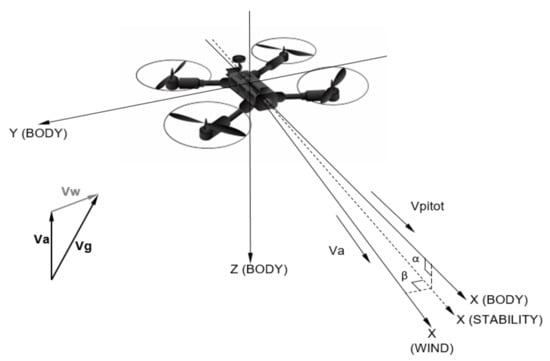
Figure 1.
Airspeed definition and wind triangle.
The wind velocity vector relative to the Earth, decomposed in the NED CF, is . The relation among the airspeed (velocity with respect to the surrounding air), the ground speed (velocity with respect to the Earth frame), and the wind velocity (with respect to the Earth frame) is:
The rotation matrix for moving from the vehicle-carried NED frame to the body frame, , is defined by roll (, positive up), pitch (, positive right), and yaw (ψ, positive clockwise) angles [27] (Chap. 2):
Therefore, the relative velocity (airspeed) vector in the body CF is:
According to [27], the airspeed vector body-frame components can be expressed in terms of the airspeed magnitude, angle of attack, and sideslip angle as:
The AOA, α, is defined as the angle between the longitudinal (X) axis of the airframe and the freestream velocity (or relative wind), measured in the Y–Z plane of the body CF, and is positive when there is uplift (pitch-up), whereas the AOS, β, is measured between the X-body axis of the airframe and the relative wind velocity vector, and is positive for wind coming from starboard (right side). Inverting Equation (5), the angles α, β and the true airspeed are given by:
The calibrated airspeed is derived from [30] (Chap. 3):
where and are the sea-level standard atmospheric values of air density and pressure, respectively (, at 15 °C, or 288.15 K [31]), and is the measured differential pressure. When Mach numbers are small (less than 0.3), Equation (8) is related to Equation (9) by:
where σ is the relative density; i.e., the ratio between the actual air density and the standard air density at sea level. For low-level flights and small velocities (typical of small UAV mission scenarios), . can be assumed as equal to .
2.2. Error Analysis
Assuming statistically independent observations, the variance of the calculated value of (Equation (6)), , can be evaluated using the special law of propagation of variances (SLOPOV) [32] (Chapter 6):
where and are the variance of the measured quantities and , respectively Equation (11) can be easily rearranged as follows:
As far as is concerned, using Equation (7) and the SLOPOV, it can be shown that:
where , and . Assuming that the vertical winds are zero (usually correct for a nonturbulent atmosphere), and measuring the sideslip angle in the X–Y plane of the body CF to maintain independence (i.e., decoupling) between and , then , , and Equation (13) can be expressed in a form similar to Equation (12):
From Equations (12) and (14), it can be seen, by finding the maxima of the functions and , that the errors in and are maximized when the velocity ratios or (for , or ) are equal to 1, and and increase as the velocity components become small; i.e., the vehicle approaches a hovering flight (in which knowledge of AOA and AOS becomes less important to the control strategy). Figure 2a, as an example, shows in degrees as a function of and , assuming a typical value of 0.2 m/s for the standard deviations of the measured velocity components ( and .
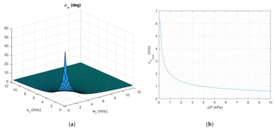
Figure 2.
(a) Standard deviation (in degrees) of the AOA, , as a function of the measured velocity components. (b) Standard deviation of the calibrated airspeed.
Finally, using Equation (9), the variance of the calibrated airspeed is found to be:
where is the variance of the differential pressure measurements ( set to 0.1 kPa; see Table 2, Section 3). Figure 2b shows the propagated error on (i.e., ) as a function of , with operating pressure range of the sensor from 0 to 10 kPa, as from Table 2.
2.3. Measurement Noise Estimation via Kalman Filtering
We applied Kalman filtering [33] for measurement noise estimation and removal, using a simple 1D formulation. The measurement process was modeled as:
where is the k-th measurement; is the (Gaussian, zero-mean) model noise with variance (initialized to 0); is the (Gaussian, zero-mean) measurement noise, with variance R, derived from the sensors’ technical datasheet (see Section 3); and A and C are scalar quantities equal to 1. The (scalar) variance of the estimation error is P.
The predictor–corrector sequence (Kalman filtering) used in our work was implemented in the Arduino Integrated Development Environment (IDE) as a function (KF_nr, where “nr” stands for “noise removal”) called whenever a new measurement (Data) was available from the sensor. The equations of the a priori estimation error, the Kalman gain , the updated estimate (with current data ), and the minimum-square a posteriori estimation error , are, respectively:
The Arduino code translated these equations (using the compound addition “+=”) as shown in Table 1.

Table 1.
The 1D Kalman filtering code implemented for measurement noise reduction.
3. Sensor System
The system used for velocity, AOA, AOS, and attitude estimation is composed of the following:
- Differential pressure sensor (Freescale Semiconductor MPX2010DP micro-Pitot);
- Static pressure sensor (Bosch Sensortec BMP180);
- IMU (DFRobot 10 DOF MEMS IMU sensor);
- Microcontroller (Arduino Mega 2560).
3.1. Differential Pressure Sensor (MPX2010DP)
Estimating the CAS (Equation (9)) requires evaluation of the dynamic pressure. The Freescale Semiconductor, Inc. MPX2010DP (Figure 3) silicon piezoresistive pressure sensor [34] provides a very accurate and linear voltage output directly proportional to the applied differential pressure, in the range of 0–10 kPa.
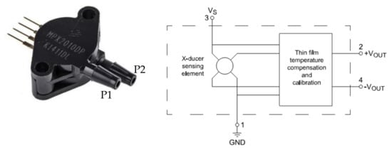
Figure 3.
The MPX2010DP differential pressure sensor and its schematics. P1 and P2 are the pressure side and the vacuum side, respectively.
The output voltage of the differential gauge sensor increases with increasing pressure applied to the positive pressure side (port P1 in Figure 3) relative to the vacuum side (port P2). The sensor is designed to operate with positive differential pressure applied (P1 > P2). Table 2 shows some technical specifications at 25 °C.
Table 2.
The main operating characteristics of the MPX2010DP.
The sensor housed a single monolithic silicon die with the strain gauge and thin film resistor network integrated. The chip was laser-trimmed for precise span, offset calibration, and temperature compensation, allowing optimal linearity, low pressure and temperature hysteresis (±0.1%VFSS from 0 to 10 kPa and ±0.5%VFSS from −40 °C to 125 °C, respectively), and an excellent response time. It fulfilled the in-flight requirements.
3.2. Digital Pressure Sensor (BMP180)
The static pressure also was acquired by the BMP180 digital pressure sensor (Figure 4) in order to obtain redundant measurements and more accurate estimates. The BMP180, produced by Bosch Sensortec, consists of a piezoresistive sensor, an analog-to-digital converter, a control unit with E2PROM, and a serial I2C interface, which allowed for easy system integration by direct connection to commercial microcontrollers [35]. The 16-bit (or 19-bit in high-resolution mode) pressure data, in the range of 300–1100 hPa (from +9000 m to −500 m related to sea level) and 16-bit temperature data were compensated by the calibration data stored in the embedded E2PROM. Detailed sensor features are reported in Table 3.
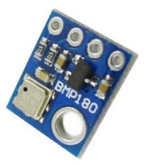
Figure 4.
The BMP180 digital pressure sensor.
Table 3.
Key features of the BMP180.
3.3. 10 DOF IMU
The DFRobot 10 DOF IMU sensor [36] (Figure 5) is a low-power (10 mW), compact-size (26x18mm) board, fully compatible with the Arduino microcontroller family, and integrates an Analog Device 10-bit ADXL345 accelerometer with up to ±16 g dynamic range, -g sensitivity, and ±40-mg drift [37]; a Honeywell HMC5883L magnetometer [38]; a 16-bit ITG-3205 gyro with ±2000°/s full-scale range, 0.014°/s sensitivity, and ±1°/s drift [39]; and a Bosch BMP085 pressure sensor. The IMU is a polysilicon surface micromachined structure built on top of a silicon wafer. Polysilicon springs suspend the structure over the surface of the wafer and provide resistance against acceleration forces.
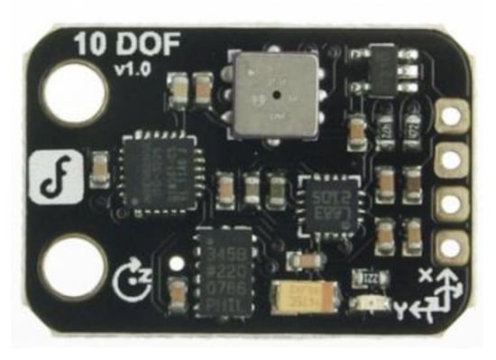
Figure 5.
The 10 DOF MEMS IMU.
IMU measurements were used in this research to estimate the acceleration components and the angular rates in Equation (1), and to check the effectiveness of the micro-Pitot approach for velocity and attitude determination.
3.4. Microcontroller
The Arduino Mega 2560 board (102 × 53 mm, weight 37 g) is a microcontroller board based on the ATmega2560. It has 54 digital input/output pins (of which 14 can be used as PWM outputs), 16 analog inputs, 4 UARTs (hardware serial ports), a 16-MHz crystal oscillator, a USB connection, a power jack, an ICSP header, and a 5 V voltage supply. The board has 250-mA current absorption (1.25-W power consumption) when running code and providing power to external sensors. The board contains everything needed to support the microcontroller; simply connecting it to a computer with a USB cable or powering it with an AC-to-DC adapter or battery allows the board be used and work in an integrated development environment (IDE) based on the Processing language project.
4. Simulations, Results, and Performance Evaluation
Schematics and a prototype of the acquisition system are shown in Figure 6 and Figure 7, respectively. The indoor experimental campaigns were performed in the PFDL of the University of Naples “Parthenope”, Naples, Italy.
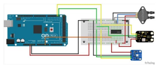
Figure 6.
Electric scheme of the developed system.
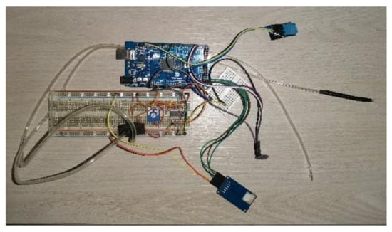
Figure 7.
Prototype of the data-acquisition system.
The system was tested using a fan as airflow generator while acquiring the differential pressures from the MPX2010DP sensor. The sensor’s measurement range is 0–1023 (10 bits). Data were collected in 3-min acquisitions at a sampling frequency of 10 Hz. A digital anemometer (Proster PST-TL017 Handheld Anemometer [40]) was used for reference measurement of the airstream. Table 4 reports some technical specifications of the PST-TL017 device, shown in Figure 8.
Table 4.
Technical data for the PST-TL017.
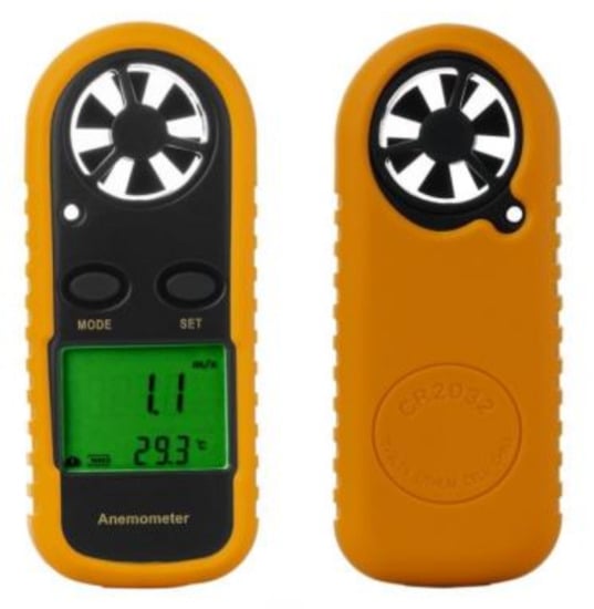
Figure 8.
The PST-TL017 anemometer used for the airflow speed check.
4.1. Pressure-Sensor Calibration
To reduce measurement noise, 1D Kalman filtering was applied to the raw data, postprocessed in the Matlab® software environment; the results are shown in Figure 9. Preliminarily, for sensor bias estimation, digital pressure data (10-bit strings) were collected in quiet airflow ().
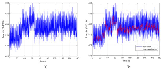
Figure 9.
(a) Raw data from the MPX2010DP, with . (b) Comparison between the raw data and the low-pass-filtered data.
The MPX2010DP sensor used the raw Arduino 5 V voltage source, and the output voltage was amplified by a two-stage differential op-amp circuit with default gains of 101 (first stage) and 6 (second stage), to obtain a signal in the range of 0–5 V. Inherent in the MPX2010 family of pressure sensors is a zero-pressure offset voltage, typically up to 1 mV. At a 5 V supply voltage, the zero-pressure offset was 0.5 mV, which corresponded to a 0.39 V offset voltage in the first op-amp stage. This offset was amplified by the second stage and appeared as a DC offset at with no differential pressure applied. Using the design considerations described in [41], at zero pressure we expected a theoretical voltage value after the second gain stage of 2.34 V, and a pressure range of 0–2 kPa. Since the supply voltage was 5 V, the available signal for the actual pressure was .
When , the sensor’s DN (digital number) average output was 477, which corresponded to (very close to the expected value), according to:
The average bias voltage acquired at (Figure 10), , was subtracted from measurements with values of to estimate the differential pressure and velocity.
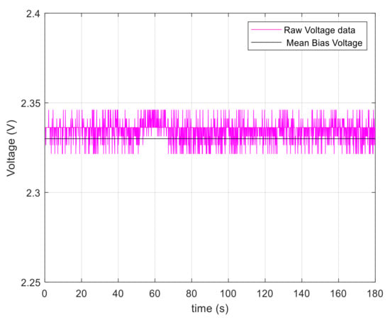
Figure 10.
The bias voltage (output at ).
To convert voltage into differential pressure (, in kPa) and evaluate the velocity from Equation (9), the following linear relation was applied:
where , , and 2 is the full scale of the sensor (2 kPa).
4.2. Indoor Tests—Velocity Estimation
The indoor experiments were performed by mounting the equipment on a test bench on which the airflow was generated by a domestic fan, placed at 0.5 m from the micro-Pitot tube. The environmental conditions were: 33% relative humidity at 27 °C, collected by the DHT11 sensor, a low-cost, small-size (12 mm × 15.5 mm, mass < 5 g), low-power (12.5-mW power consumption when operating at 5 V, 2.5 mA) temperature and humidity sensor with a calibrated 16-bit digital signal output on a single-wire serial interface, with a 20–80% relative humidity range (accuracy 5%) and 0–50 °C temperature range with ± 2 °C accuracy [42].
Three airflow conditions were set as follows:
- Speed 0: 0 m/s (for system calibration);
- Speed 1: m/s (measured by the anemometer);
- Speed 2: randomly varying airflow.
Data were acquired at a 10 Hz sampling rate. Bias estimation and sensor calibration (Section 4.1) were performed in the “Speed 0” condition. Figure 11 and Figure 12 show the acquired raw (unfiltered) and filtered data in the “Speed 1” and “Speed 2” (random wind speed) conditions, respectively. As a check of the effectiveness of the calibration strategy, the average estimated velocity value in the “Speed 1” test condition (Figure 11) was found to be 2.56 m/s; this corresponded to a relative error equal to . Raw data smoothing was performed as shown in Figure 11a and Figure 12a with a moving average filter (the Matlab function smoothdata) in the time domain, comparable (but not as effective) to low-pass filtering in the frequency domain, while Figure 11b and Figure 12b show the effect of 1D KF on the processed data.
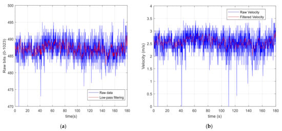
Figure 11.
(a) Raw data collection during the “Speed 1” test. (b) Velocity acquisition (raw data vs. KF data) calculated by Equation (9).
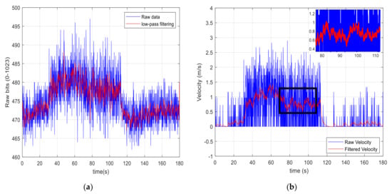
Figure 12.
(a) Raw data vs. low-pass-filtered data (DN of sensor measurement). (b) Raw data vs. KF data (calculated velocity) in test condition “Speed 2”.
4.3. Indoor Tests—AOA, AOS, and Attitude Estimation
AOA and AOS were calculated according to Equations (5) and (6). The entire system was successively mounted on a movable structure (Figure 13) to simulate various attitude changes of the UAV during the indoor tests. The following assumptions were made:
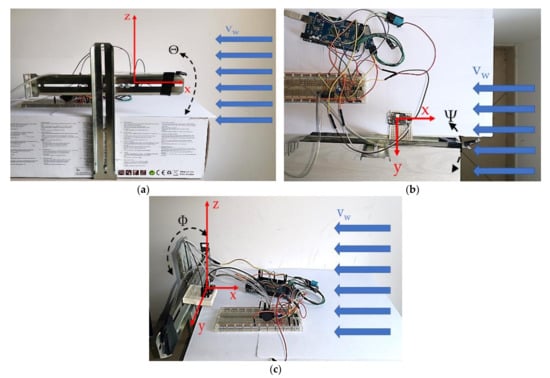
Figure 13.
The prototype mounted on a movable structure to simulate pitch (a), yaw (b), and roll (c) variations.
- Static data acquisition: the system was fixed and simply surrounded by the constant airflow coming from the fan;
- Pitot tube aligned with the airframe longitudinal axis: the relative velocity was equal to the airflow velocity, and from Equation (4):
Several test cases were set up, as shown in Table 5, in which the actual wind velocity () was measured by the digital anemometer, and the controlled (“true”) attitude angles were selected by using a graduated scale mounted on the structure. For example, in test case 1, the system was set in a horizontal position, with the X–Y plane parallel to the ground (yaw, roll, and pitch angles equal to 0°, calculated by the IMU), and the “true” wind velocity was set to 7 m/s.
Table 5.
The test cases and parameter setup.
To estimate roll and pitch angles from the IMU, a complementary filter was applied, fusing accelerometer and gyroscope data, to reduce drift and noise errors [43,44]:
where are the estimates of roll, pitch, and yaw angles at the instant k; is the filter coefficient; is the angular rate vector derived from gyroscopic measurements [45]; and are the angles derived from the accelerometer data vector . These can be derived from triple-axis tilt calculation, which evaluates the angles between the gravity vector and the accelerometer’s z-axis (with positive direction opposite to gravity); between the horizon (initially coincident with the accelerometer xy-plane) and the x-axis, coincident with the body longitudinal axis; and between the horizon and the y-axis of the accelerometer [46]:
The roll angle () is given by , and pitch () is given by . The yaw angle was estimated by simply integrating the gyroscopic yaw rate. The filter coefficient was determined by:
where τ is the time constant of the filter. Figure 14 shows the KF velocity estimation and the Euler angles with the complementary filter during data collection in static conditions (test case 1).
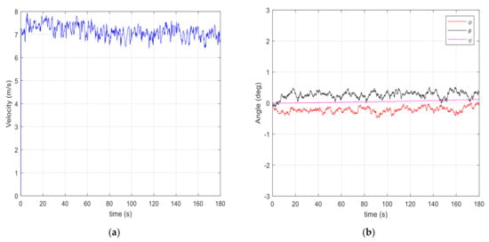
Figure 14.
(a) The filtered velocity measured by the differential pressure sensor in test case 1. (b) The Euler angles after complementary filtering (fusion of gyroscope and accelerometer data from the IMU).
Following Equation (4), the relative velocity and its components were evaluated, whereas Equations (6) and (7) were used to estimate the AOA (α) and AOS (β). Table 6 shows the average values of the estimates and the experimental results for the seven test cases devised, and Figure 15, Figure 16, Figure 17 show the collected data and the estimates during test conditions 3, 6, and 7, respectively.
Table 6.
Estimates of , AOA, and AOS in the seven experimental setups (filtered data).
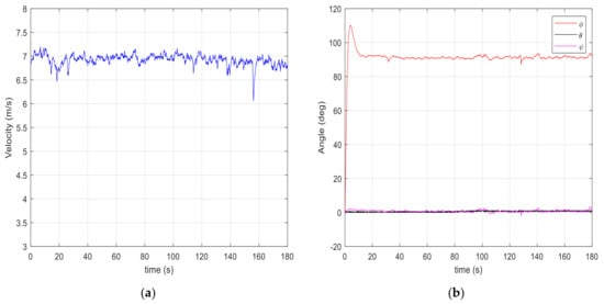
Figure 15.
The filtered velocity (a) and yaw, pitch, and roll angles (b) during test case 3.
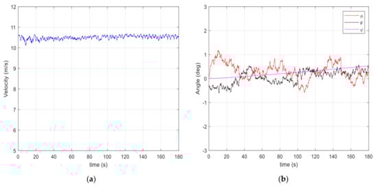
Figure 16.
The filtered velocity (a) and filtered Euler angles (b) during test case 6.
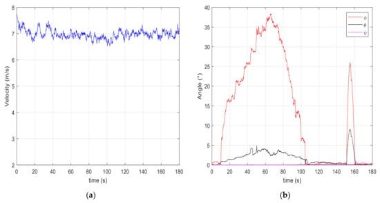
Figure 17.
Data collection in dynamic conditions (test case 7, simulation of a roll variation from 0–40°). (a) filtered velocity, (b) filtered Euler angles.
A simple statistical analysis was conducted on the estimates of airspeed, AOA, and AOS to evaluate the system’s performance. Table 7 shows the standard deviations of the estimated values ( and before and after filtering), while Figure 18 shows a plot of and as a function of the velocity magnitude, together with the relative least-square fits. The experimental data were in agreement with the growth in errors as the velocities approached zero, according to the developed error analysis (Section 2.2).
Table 7.
Standard deviations of estimated CAS, AOA, and AOS (raw and filtered data).
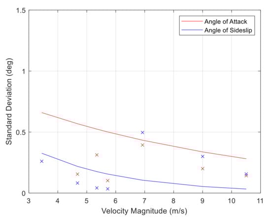
Figure 18.
The standard deviation of the angle of attack and sideslip vs. magnitude of the relative velocities: numerical values and least-square fit.
5. Conclusions and Further Work
This paper presented a kinematic model for estimation of airspeed, angle of attack α, and sideslip angle β for small UAVs equipped with low-cost, off-the-shelf commercial navigation sensors. The devised system used a miniaturized differential pressure sensor (micro-Pitot tube) and an IMU for attitude determination, managed by a microcontroller. The calibration technique used for the pressure sensor returned estimation errors of less than 3%. The system performance was evaluated using experimental results from indoor benchmarking tests that emulated some basic dynamics of typical UAV missions. As shown in Table 6, the relative error that affected airspeed measurements was found to be less than 9% in all the test scenarios considered, or less than 5% if we excluded test case 4 shown in Table 6, relative to a nonrealistic value of the AOA (which was typically in the range of −2° to 15°). The estimation errors of α, β, and were found to be within 1.7° (excluding the nonrealistic case ), 0.5°, and 1.4 m/s, respectively, in good agreement with the theoretical values derived from the law of error propagation, and consistent with other authors’ work [15,19,20,26]. The proposed approach showed a promising potentiality for implementation of real-time control laws to increase the flight envelope by exploiting attitude measurements and direct knowledge of α and β. Using AOA and AOS estimates as in-flight feedback inputs to the autopilot control loop also could help to improve the endurance of small aircraft (typically in the range 15–45 min) by implementing specific flight strategies according to the wind conditions, or even optimizing the trajectory by gaining power in energy-harvesting techniques. There are, however, some limitations of the proposed methodology:
- The alignment of the micro-Pitot tube (differential pressure sensor) to the longitudinal axis of the UAV must be performed very precisely in order to avoid biases in the estimations of the AOA and AOS. Moreover, the sensor must be located reasonably far from the rotary wings (considering a quadcopter or a multirotor VTOL UAV) to avoid turbulent airflow added by the rotors.
- High velocities (>20 m/s) create differential pressure values out of the available sensor range (0.10 kPa at 10 V supply, 0–2 kPa at 5 V supply). This was not an issue for the micro-UAV applications devised by the authors (the system will be installed on a quadcopter with maximum velocity on the order of 10 m/s), but could be a problem for larger aircraft.
- The mass and size requirements of our system (<150 g, typical dimensions of the boxed prototype of 120 × 60 × 30 mm) fit typical mini- and micro-UAV payload constraints, but the power consumption of the system (in the range 1–2W) could significantly reduce the aircraft’s endurance (which was in the order of 15–30 min for typical small UAVs). Therefore, careful engineering considerations must be devised to reduce the impact of the system in terms of flight mission duration.
Future work will involve the realization of a minimum-size, minimum-weight version of the sensor suite, to be strapdown-mounted on a small UAV with a 2 kg maximum take-off weight (MTOW); the implementation of outdoor tests in typical flight and atmospheric conditions; and further developments of the error models and the attitude kinematics, to improve the accuracy of airflow angle and sideslip estimates in various flight and wind conditions.
Author Contributions
Conceptualization, methodology, G.A., S.P., and U.P.; software and validation, G.A., S.P., and U.P.; formal analysis, investigation, data curation, G.A., S.P., and U.P.; resources, G.D.C.; writing—original draft preparation, G.A., U.P., and S.P.; writing—review and editing, S.P.; supervision, funding acquisition, G.D.C. All authors have read and agreed to the published version of the manuscript.
Funding
This work was supported by the University of Naples “Parthenope” (Italy) Internal Research Project DIC (Drone Innovative Configurations, CUP I62F17000060005-DSTE 338).
Acknowledgments
The authors wish to thank Alberto Greco for his invaluable support during the laboratory tests, and the four anonymous reviewers who helped them to enhance the scientific and technical content of the paper with their enlightening observations.
Conflicts of Interest
The authors declare no conflict of interest.
References
- U.S. Army UAS Center of Excellence (ATZQ-CDI-C). Eyes of the Army”—U.S. Army Roadmap for Unmanned Aircraft Systems 2010–2035; Army UAS CoE Staff: Fort Rucker, AL, USA, 2010. [Google Scholar]
- Papa, U. Embedded Platforms for UAS Landing Path and Obstacle Detection. In Studies in Systems, Decision and Control; Springer: New York, NY, USA, 2018; Volume 136. [Google Scholar]
- Nawaz, H.; Ali, H.M.; Massan, S.-U. Applications of unmanned aerial vehicles: A review. 3c Tecnol. 2019. [Google Scholar] [CrossRef]
- González-Jorge, H.; Martínez-Sánchez, J.; Bueno, M.; Arias, A.P. Unmanned aerial systems for civil applications: A review. Drones 2017, 1, 2. [Google Scholar] [CrossRef]
- Shakhatreh, H.; Sawalmeh, A.H.; Al-Fuqaha, A.; Dou, Z.; Almaita, E.; Khalil, I.; Othman, N.S.; Khreishah, A.; Guizani, M. Unmanned Aerial Vehicles (UAVs): A survey on civil applications and key research challenges. IEEE Access 2019, 7, 48572–48634. [Google Scholar] [CrossRef]
- ENAC (Ente Nazionale per l’Aviazione Civile). Regolamento Mezzi aerei a pilotaggio remoto. Amendment 1, 14/07/2020; Enac: Rome, Italy, 2020. [Google Scholar]
- Abdelkrim, N.; Aouf, N. Robust INS/GPS sensor fusion for UAV localization using SDRE nonlinear filtering. IEEE Sens. J. 2010, 10, 789–798. [Google Scholar]
- Gross, J.N.; Gu, Y.; Rhudy, M.B.; Gururajan, S.; Napolitano, M.R. Flight-test evaluation of sensor fusion algorithms for attitude estimation. IEEE Trans. Aerosp. Electron. Syst. 2012, 48, 2128–2139. [Google Scholar] [CrossRef]
- Yang, X.; Mejias Alvarez, L.; Garratt, M. Multi-sensor data fusion for UAV navigation during landing operations. In Proceedings of the Australasian Conference on Robotics and Automation (ACRA 2011), Australian Robotics and Automation Association, Melbourne, Australia, 7–9 December 2011. [Google Scholar]
- Del Pizzo, S.; Papa, U.; Gaglione, S.; Troisi, S.; Del Core, G. A vision-based navigation system for landing procedure. Acta IMEKO 2018, 7, 102–109. [Google Scholar] [CrossRef]
- Ariante, G.; Papa, U.; Ponte, S.; Del Core, G. UAS for positioning and field mapping using LIDAR and IMU sensors data: Kalman filtering and integration. In Proceedings of the IEEE 5th International Workshop on Metrology for AeroSpace (MetroAeroSpace), Turin, Italy, 19–21 June 2019. [Google Scholar]
- Wang, B.H.; Wang, D.B.; Ali, Z.A.; Ting, B.T.; Wang, H. An overview of various kinds of wind effects on unmanned aerial vehicle. Meas. Control. 2019, 52, 731–739. [Google Scholar] [CrossRef]
- Tian, P.; Chao, H.; Rhudy, M.; Gross, J.; Wu, H. Wind sensing and estimation using small fixed-wing unmanned aerial vehicles: A survey. J. Aerosp. Inf. Syst. 2021, 18, 132–143. [Google Scholar] [CrossRef]
- Shimura, T.; Inoue, M.; Tsujimoto, H.; Sasaki, K.; Iguchi, M. Estimation of wind vector profile using a hexarotor unmanned aerial vehicle and its application to meteorological observation up to 1000 m above surface. J. Atmos. Ocean. Technol. 2018, 35, 1621–1631. [Google Scholar] [CrossRef]
- Petrich, J.; Subbarao, K. On-board wind speed estimation for Uavs. In Proceedings of the AIAA Guidance, Navigation, and Control Conference, Portland, OR, USA, 8–11 August 2011. [Google Scholar]
- Watkins, S.; Milbank, J.; Loxton, B.J.; Melbourne, W.H. Atmospheric winds and their implications for microair vehicles. AIAA J. 2006, 44, 2591–2600. [Google Scholar] [CrossRef]
- Langelaan, J.W.; Alley, N.; Neidhoefer, J. Wind field estimation for small unmanned aerial vehicles. J. Guid. Control. Dyn. 2011, 34, 1016–1030. [Google Scholar] [CrossRef]
- Gavrilovic, N.; Benard, E.; Pastor, P.; Moschetta, J.-M. Performance improvement of small UAVs through energy-harvesting within atmospheric gusts. In Proceedings of the AIAA SciTech Forum, Grapevine, TX, USA, 9–13 January 2017. [Google Scholar]
- Johansen, T.A.; Cristofaro, A.; Sorensen, K.; Hansen, J.M.; Fossen, T.I. On estimation of wind velocity, angle-of-attack and sideslip angle of small UAVs using standard sensors. In Proceedings of the International Conference on Unmanned Aircraft Systems (ICUAS), Denver, CO, USA, 9–12 June 2015. [Google Scholar]
- Perry, J.; Mohamed, A.; Johnson, B.; Lind, R. Estimating angle of attack and sideslip under high dynamics on small UAVs. In Proceedings of the ION GNSS 21st International Technical Meeting of the Satellite Division, Savannah, GA, USA, 16–19 September 2008; pp. 1165–1173. [Google Scholar]
- Sankaralingam, L.; Ramprasadh, C. A comprehensive survey on the methods of angle of attack measurement and estimation in UAVs. Chin. J. Aeronaut. 2019, 33, 749–770. [Google Scholar] [CrossRef]
- Ramprasadh, C.; Prem, S.; Sankaralingam, L.; Deshpande, P.; Dodamani, R. A simple method for estimation of angle of attack. IFAC-Pap. 2018, 51, 353–358. [Google Scholar] [CrossRef]
- Ramprasadh, C.; Arya, H. Multistage-fusion algorithm for estimation of aerodynamic angles in mini aerial vehicle. J. Aircr. 2012, 49, 93–100. [Google Scholar] [CrossRef]
- Ariante, G.; Papa, U.; Ponte, S.; Del Core, G. Velocity and attitude estimation of a small unmanned aircraft with micro Pitot tube and Inertial Measurement Unit (IMU). In Proceedings of the IEEE 7th International Workshop on Metrology for Aerospace (MetroAer-oSpace), Pisa, Italy, 22–24 June 2020. [Google Scholar]
- De Marina, H.G.; Pereda, F.J.; Giron-Sierra, J.M.; Espinosa, F. UAV attitude estimation using unscented Kalman filter and TRIAD. IEEE Trans. Ind. Electron. 2011, 59, 4465–4474. [Google Scholar] [CrossRef] [Green Version]
- Zhang, Q.; Xu, Y.; Wang, X.; Yu, Z.; Deng, T. Real-time wind field estimation and pitot tube calibration using an extended Kalman filter. Mathematics 2021, 9, 646. [Google Scholar] [CrossRef]
- Beard, R.W.; McLain, T.W. Small Unmanned Aircraft: Theory and Practice; Princeton University Press: Princeton, NJ, USA, 2012. [Google Scholar]
- Cai, G.; Chen, B.M.; Lee, T.H. An overview on development of miniature unmanned rotorcraft systems. Front. Electr. Electron. Eng. China 2009, 5, 1–14. [Google Scholar] [CrossRef]
- Quan, Q. Introduction to Multicopter Design and Control; Springer: Singapore, 2017. [Google Scholar]
- Yechout, T.; Morris, S.L.; Bossert, D.E.; Hallgren, W.F. Introduction to aircraft flight mechanics: Performance, static stability, dynamic stability, and classical feedback control. In AIAA Education Series; American Institute of Aeronautics and Astronautics, Inc.: Reston, VA, USA, 2003. [Google Scholar]
- International Organization for Standardization (ISO). Standard Atmosphere; ISO: London, UK, 1975. [Google Scholar]
- Ghilani, C.D. Adjustment Computations—Spatial Data Analysis, 5th ed.; John Wiley and Sons, Inc.: Hoboken, NJ, USA, 2010. [Google Scholar]
- Grewal, M.S.; Andrews, A.P. Kalman Filtering—Theory and Practice Using MATLAB®, 3rd ed.; John Wiley and Sons, Inc.: Hoboken, NJ, USA, 2008. [Google Scholar]
- NXP B., V. MPX2010 Series—10 kPa Temperature Compensated Pressure Sensors—Product Datasheet. Rev. 14. 2021. Available online: https://www.nxp.com/docs/en/data-sheet/MPX2010.pdf (accessed on 1 July 2021).
- Bosch Sensortec. BMP180 Digital Pressure Sensor, Rev. 2.8, Doc. No. BST-BMP180-DS000-12. 2015. Available online: https://git.wapakema.de/walter/Wetterstation/raw/commit/5d7e482b2baaa35a205b06021f282d10bd271cd3/python/BMP280.pdf (accessed on 1 July 2021).
- DFRobot, 2018. 10-Dof MEMS IMU Sensor V2.0. Available online: https://www.dfrobot.com/wiki/index.php/10_DOF_Mems_IMU_Sensor_V2.0_SKU:_SEN0140 (accessed on 1 July 2021).
- Analog Devices. Small, Low Power, 3-Axis ±3g Accelerometer ADXL335-345. Rev. 0; One Technology Way: Norwood, MA, USA, 2009. Available online: https://www.sparkfun.com/datasheets/Components/SMD/adxl335.pdf (accessed on 1 July 2021).
- Honeywell. 3-Axis Digital Compass IC HMC5883L. Rev E.; Honeywell: Plymouth, MN, USA, 2013. [Google Scholar]
- InvenSense Inc. ITG-3200 Product Specification—Revision 1.7; InvenSense Inc.: Sunnyvale, CA, USA, 2011. [Google Scholar]
- Proster®. Proster TL017 Handheld Anemometer Wind Speed Meter Scale Gauge. 2012. Available online: http://www.prostereu.com/index.php/2015/07/24/tl017/ (accessed on 1 July 2021).
- Romero, M.; Figueroa, R. Low-Pressure Sensing Using MPX2010 Series Pressure Sensors. Application Note AN4010, Rev. 1; Freescale Semiconductors Inc.: Austin, TX, USA, 2005. [Google Scholar]
- Adafruit Industries. DHT11, DHT22 and AM2302 Sensors. 2020. Available online: https://cdn-learn.adafruit.com/downloads/pdf/dht.pdf (accessed on 3 September 2021).
- Merhav, S. Aerospace Sensor Systems and Applications; Springer: New York, NY, USA, 1996. [Google Scholar]
- Gui, P.; Tang, L.; Mukhopadhyay, S. MEMS based IMU for tilting measurement: Comparison of complementary and Kalman filter based data fusion. In Proceedings of the IEEE 10th conference on Industrial Electronics and Applications (ICIEA), Auckland, New Zealand, 15–17 June 2015. [Google Scholar]
- Stančin, S.; Tomazic, S. On the interpretation of 3D gyroscope measurements. J. Sens. 2018, 2018, 1–8. [Google Scholar] [CrossRef] [Green Version]
- Fisher, C.J. Using an Accelerometer for Inclination Sensing. AN-1057 Application Note; Analog Devices Inc.: Norwood, MA, USA, 2010. [Google Scholar]


Publisher’s Note: MDPI stays neutral with regard to jurisdictional claims in published maps and institutional affiliations. |
© 2021 by the authors. Licensee MDPI, Basel, Switzerland. This article is an open access article distributed under the terms and conditions of the Creative Commons Attribution (CC BY) license (https://creativecommons.org/licenses/by/4.0/).