Abstract
The localization of electromagnetic interference (EMI) sources is of high importance in electromagnetic compatibility applications. Recently, a novel localization technique based on the time-reversal cavity (TRC) concept was proposed using only one sensor, and its application to localize EMI sources was validated numerically. In this paper, we present a validation of the proposed time-reversal process in which the forward step of the time-reversal process is performed experimentally and the backward step is carried out via numerical simulations, a realistic scenario which is applicable to practical source localization problems. To the best of the authors’ knowledge, this is the first implementation of a three-dimensional electromagnetic time-reversal process in which the forward signal is provided experimentally while the backward propagation step is carried out numerically. The considered experimental setup is formed by a partially open cavity and two monopole antennas to emulate the EMI source and the sensor (receiving antenna), respectively. Assuming that the location of the source is the feed point of the monopole antenna, the resulting three-dimensional location error in the experimental validation was only 1.49 cm, which is about one-third the length of the monopole antenna, corresponding to about λmin/2 (diffraction limit).
1. Introduction
The localization of electromagnetic interference (EMI) sources from electronic devices, printed circuit boards, cables, and natural electromagnetic sources is important in electromagnetic compatibility [1,2,3,4].
Recently, the application of the electromagnetic time-reversal (EMTR) technique [5,6,7,8,9,10] to locate electromagnetic sources has received much attention [11,12,13,14,15,16,17,18,19,20,21,22,23]. In the EMTR technique, the electromagnetic signals emitted by the source are recorded by at least one sensor. This procedure is referred to as the forward propagation phase. In the next step, called the backward propagation phase, the recorded signals are time reversed and back injected into the medium. It has been demonstrated that the back-injected waves will refocus both in time and space at the primary source location. A suitable criterion is used to localize the focal point, which corresponds to the source.
The first experimental validation of the EMTR concept was performed by Lerosey et al. [8]. In [8], to avoid the use of high-speed (GHz) digitizers, only the baseband signal (the envelope of the whole used signal) was time reversed. Furthermore, both the forward and the backward propagation phases were carried out experimentally. To provide proof of the EMTR concept, Lerosey et al. [8] considered only two locations in the backward propagation step: the real location, and a second one several wavelengths away. Their experimental data showed that the back-injected waves converge to the transmitting antenna both in time and space [8].
Based on Lerosey et al.’s investigations [8], a novel approach was proposed to localize EMI sources based on the concept of the time-reversal cavity [14]. In the new approach, the device under test (DUT) was placed inside a metallic cavity and a single monopole antenna was used to record the EMI signals emitted by the DUT. The entropy criterion [23] was applied to obtain the focusing time slice in which the maximum electric field power determines the location of the EMI source. In [14], it was shown that the reflections from the surfaces of a cavity can emulate an infinite number of sensors in the time-reversal method. The idea presented in [14] was later successfully applied to the localization of partial discharges (PDs) in power transformers [24,25,26]. The method was also found to be robust against variations in the polarization and length of the PDs and also against environmental noise. In [27], the maximum power (or field) criterion is proposed to identify the location of the EMI or partial discharge sources.
To the best of the authors’ knowledge, all the previous experimental studies aiming at validating the EMTR technique have been carried out experimentally in both the forward and the backward propagation steps. In this paper, we present, for the first time, an experimental validation of the time-reversal procedure to locate EMI sources in which the forward step signals are measured in an experimental setup and the backward phase is implemented through software simulation. Such an implementation of the time-reversal process corresponds to practical scenarios in which the back-propagation process should be performed numerically.
The paper is organized as follows. Section 2 presents the methodology of the proposed single sensor EMTR method to localize the EMI source. A description of the experimental setup and computational model used in this paper is given in Section 3. Finally, discussion and conclusions are given in Section 4.
2. Methodology
Determining the EMI source location using the EMTR method includes four steps:
Recording the emitted electromagnetic signal from one or several EMI sources with one or several sensors (forward step);
Processing the recorded signal at each sensor to time reverse it;
Back injecting the time-reversed signal into the medium (back-propagation step);
Applying a criterion to obtain the proper source location. In a real-life application of EMTR, the forward step is carried out experimentally using an antenna (sensor) and the backward step is carried out numerically.
We will consider a partially open cavity as the medium and two monopole antennas to emulate, the EMI source and the sensor (receiving antenna), respectively. In the backward propagation step, the wave converges back to the source location through an infinite number of paths as a result of reflections from the cavity surfaces [14]. This leads to an important difference between the location by EMTR in a cavity and in free space. In the free space case, the 1/R attenuation of the field needs to be removed artificially in the back-propagation step to ensure that signals exhibit the highest amplitude at the source location [13,23]. In contrast, in the case of the cavity, the attenuation function can be retained since it does not alter the refocusing of the wave back to the source due to the contribution of all the waves from multiple propagation paths. In this case, however, it is still necessary to remove the local field maxima at the location of the sensor(s) (see [14] for more details).
2.1. The Geometry of the Problem
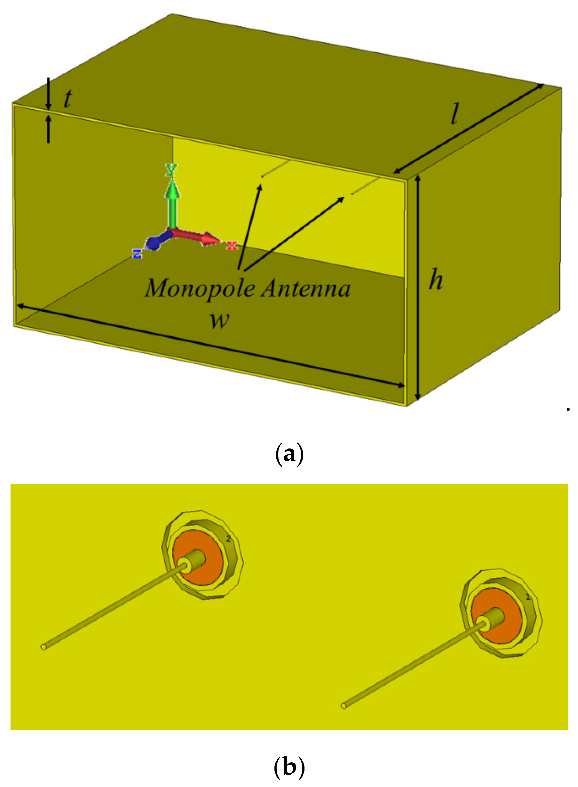
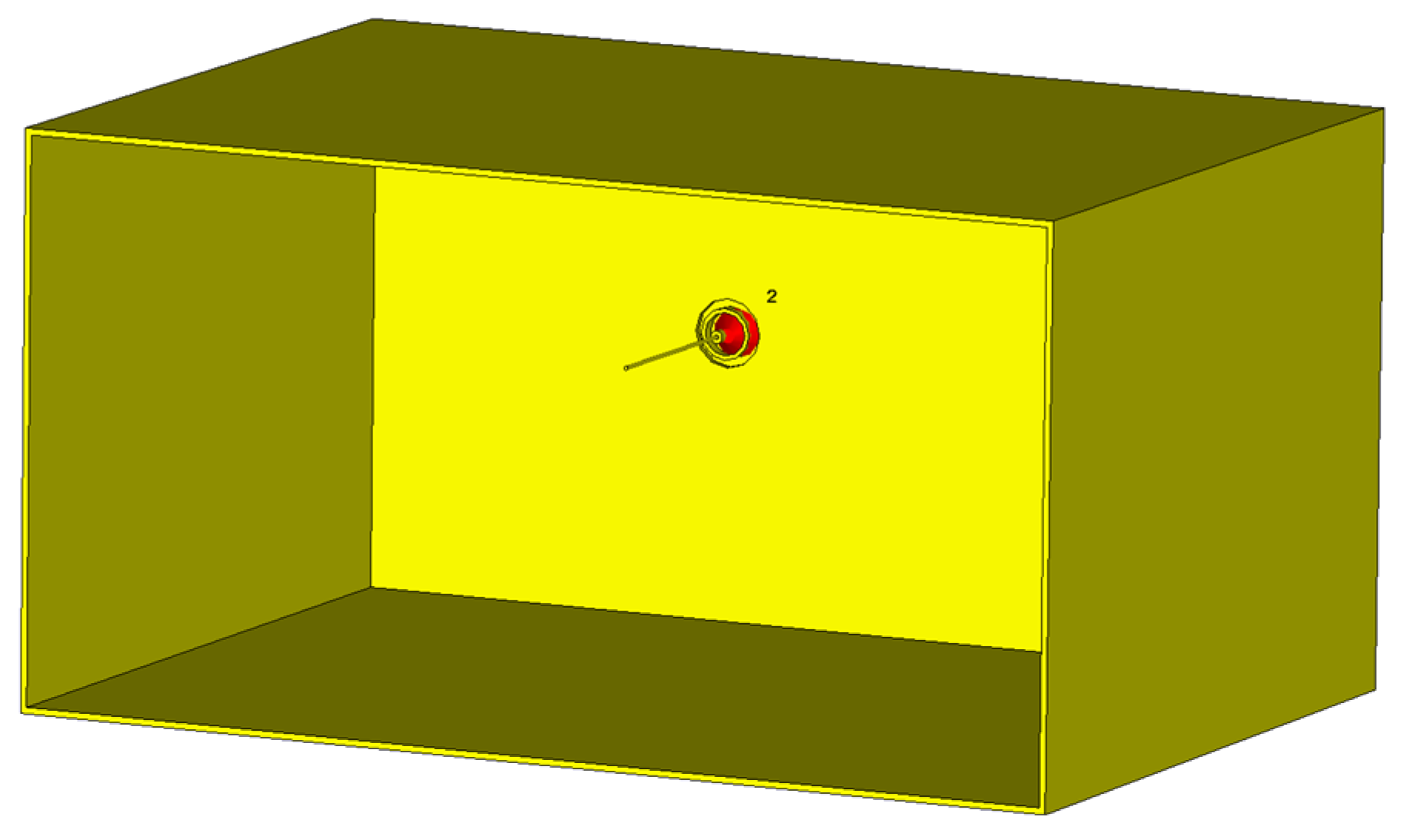
Herein, the method presented in [14] is applied to an open cavity structure. The geometry of the problem is a 3D open rectangular cavity (w = 0.25 m, l = 0.174 m, and h = 0.13 m) made of copper with a thickness of 1.5 mm, as illustrated in Figure 1. Two identical 3.5 cm long monopole antennas made of copper represent the source (right monopole antenna) and the transducer (left monopole antenna).
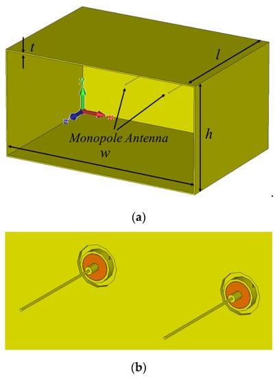
Figure 1.
Open cavity. (a) Geometry of the 3D problem, including an open metallic cavity and two monopole antennas. The dimensions of the cavity are w = 25 cm, h = 13 cm, l = 17.4 cm, and t = 1.5 mm. (b) An expanded view of the two monopoles. The left and right monopoles are considered as the sensor and the source, respectively, in the EMTR method. The two monopole antennas are identical, with a length of 5.3 cm.
An expanded view of the two-monopole antennas is depicted in Figure 1b. The transducer and the source center positions are (8.96 cm, 6.66 cm) and (14.78 cm, 6.66 cm), respectively, in the x–y plane. The location of the EMI source antenna is in the Fresnel region (1.94λ at the maximum frequency (10 GHz) of the excitation bandwidth) of the sensor. The N-type connectors attached to the antennas are assumed to be lossless and with a relative dielectric permittivity of 2.25. The length of both antennas is 5.3 cm and they are made of copper (σ = 5.8 × 10⁷ S/m). The material is modeled as copper (annealed) using the predefined material library in CST MWS.
2.2. Description of the Experimental Setup
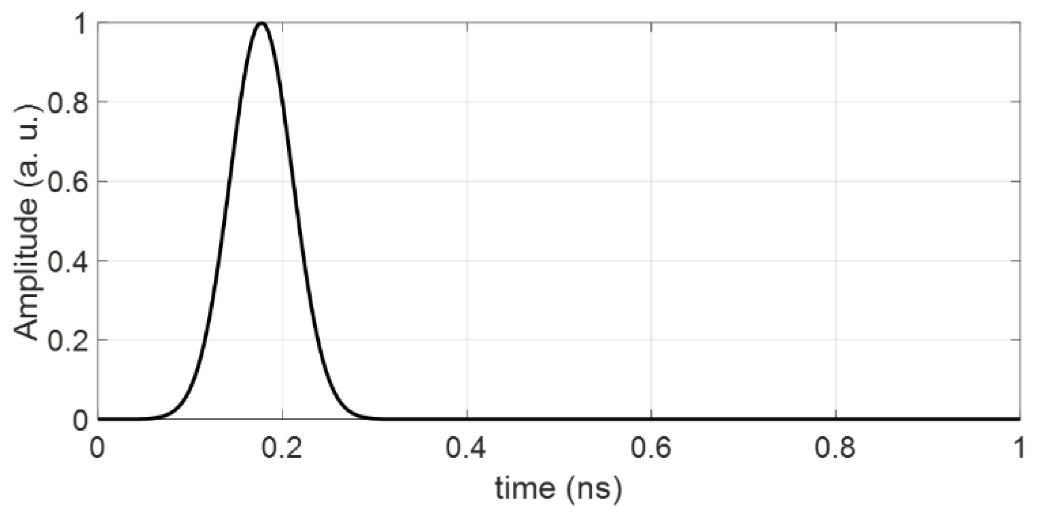
As mentioned in Section 1, in this study, the forward step in the EMTR technique is carried out experimentally. We used a vector network analyzer (VNA) in the range of 10 MHz–10 GHz to record the scattering parameter between the two monopole antennas in the frequency domain. The recorded scattering parameter is multiplied by the Fourier transform of the excitation signal (the Gaussian pulse shown in Figure 2 and the result is transformed into the time domain using the inverse Fourier transform.
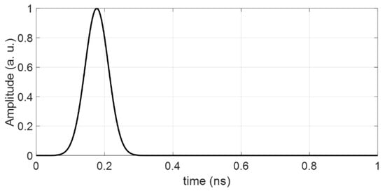
Figure 2.
Gaussian pulse with a bandwidth of 0 to 10 GHz that was used.
Pictures of the open cavity used in the experimental setup are presented in Figure 3. To emulate the open boundary condition in the test environment, we placed an absorber in front of the open side of the cavity, as shown in Figure 3a. The working frequency of the absorbers is from 1 to 40 GHz. In this range, the maximum reflectivity of the absorbers is −24 dB. The two monopole antennas shown in the expanded view in Figure 3d are connected to the VNA from the back side of the open cavity as shown in Figure 3b. It should be noted that the calibration of the VNA was performed from the end of these connectors. Figure 3c shows a front view of the open cavity to illustrate the location of the two monopole antennas. The origin and the axes of the selected coordinate system can be seen in Figure 1.
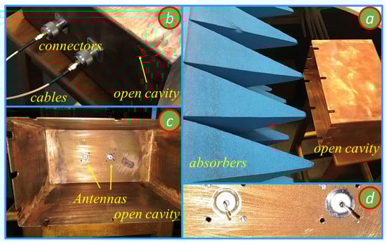
Figure 3.
Test setup including the open cavity, absorber, connectors, cables, and two monopole antennas. (a) The open cavity placed in front of the absorbers to reduce the effects of reflections from the environment on the experimental results. (b) The cables and connectors used to connect the two monopole antennas to the VNA. (c) A front view of the open cavity, including the two monopole antennas inside it, and (d) an expanded view of the two monopole antennas.
2.3. Numerical Simulation
The back-propagation step in the EMTR technique was simulated using the commercial time domain electromagnetic solver CST Microwave Studio (CST MWS). To conduct this, the time-reversed version of the signal that was obtained in the forward step was back injected by simulation through the transducer in the CST MWS model of the open cavity. As we do not know the location of the EMI source in a practical problem, we removed the transmitter antenna in the back-propagation model as shown in Figure 4. The maximum electric field power criterion was used to localize the EMI source [27].
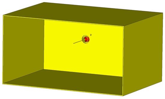
Figure 4.
Open cavity without transmitter antenna used in the back-propagation phase. Geometry of the 3D problem.
The transient solver of the CST MWS software was used to simulate the electromagnetic wave propagation inside the open cavity. This solver uses the finite integration technique (FIT) to solve Maxwell’s equations in their integral form.
A frequency range of 0 to 10 GHz was considered. The number of mesh cells was 2,572,980, the time step was 1.18 ps, and the total solver times for the forward and backward steps in CST MWS were 995 s and 1233 s, respectively. Note that the simulation time for the backward step is longer than in the forward step because the electric fields throughout the working volume need to be recorded in the backward step. All simulations were conducted on a laptop (Intel core i9 and 32 GB RAM).
3. Numerical and Experimental Results
In this section, the time-reversal process, including both the forward and backward time steps, was performed using the time domain numerical simulation. Second, to validate the numerical results, the scattering parameter S21 (see e.g., [28]), obtained by the CST MWS software was compared with the experimental data. Finally, a practical implementation of the time-reversal process was performed, in which the forward step was carried out experimentally and the backward step numerically. The simulation model and the experimental setup were described in Section 2. In what follows, we will first consider a case in which we perform all the steps in the EMTR process numerically (Section 3.1). Then, we present the validation of the model for the back-propagation step in Section 3.2. Finally, the experimental validation is presented in Section 3.3.
3.1. Numerical Simulations
In accordance with the procedure described in Section 2, the source monopole antenna shown in Figure 1 was excited using a Gaussian pulse. The propagation of the signal in the open cavity was modelled using the full-wave CST MWS simulator. The signal received by the monopole antenna was recorded and time reversed. In the back-propagation phase, the geometry of the problem in CST MWS was updated by removing the source as shown in Figure 4. Then, the time-reversed signal was back injected into the medium using the same monopole antenna. The location of the source was determined using the maximum electric field power as criterion [27]. For more information on different criteria to locate the source, please refer to [14]. It should be noted that all the procedures in the numerical simulations are carried out in the time domain.
The distribution of the normalized maximum electric field power over the computational domain and over the whole time window was obtained. Figure 5 shows the distribution at the z = 1 cm cut plane, where the overall maximum field occurs as discussed below. As can be seen, the maximum power criterion can be used to estimate the location of the EMI source. It should be noted that we removed the location ambiguity due to the presence of the sensor (at whose position the power is maximum) by introducing a square mask to ignore the values of the power around the source [27]. More details about using the mask to localize the appropriate EMI source can be found in [27]. In the considered simulations, the size of the mask was 3.4 × 3.4 cm2. In Figure 5, the black cross shows the global maximum power, which occurs at the z = 1 cm cut plane. The red circle, which is considered to be the location of the source, is the intersection between the z = 1 cm cut plane and the monopole antenna, 1 cm away from the feeding point. The localization error, defined as the distance between the center of the red circle and the black cross in the z = 1 cm cut plane, is 0.18 cm. If the feeding point is used as the location of the source, the error (the distance between the feeding point and the point of global maximum power) is 1.02 cm.
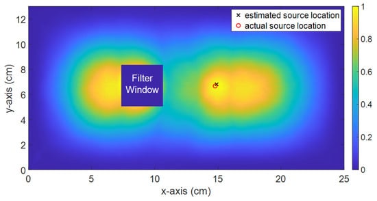
Figure 5.
Distribution of the normalized maximum power at the z = 1 cm cut plane in absence of the transmitter monopole antenna in the backward propagation step. The black cross shows the global maximum power, which occurs on the z = 1 cm cut plane. The red circle is the intersection between the z = 1 cm cut plane and the monopole antenna. The estimated location error, defined as the two-dimensional distance between the red circle and the black cross, is 0.18 cm. If the error is measured as the three-dimensional distance from the black cross to the antenna feeding point, it equals 1.02 cm. The blue square with side length of 16 cells (3.4 cm) at the location of the sensor shows the mask filter that was used in this simulation.
3.2. Model Validation
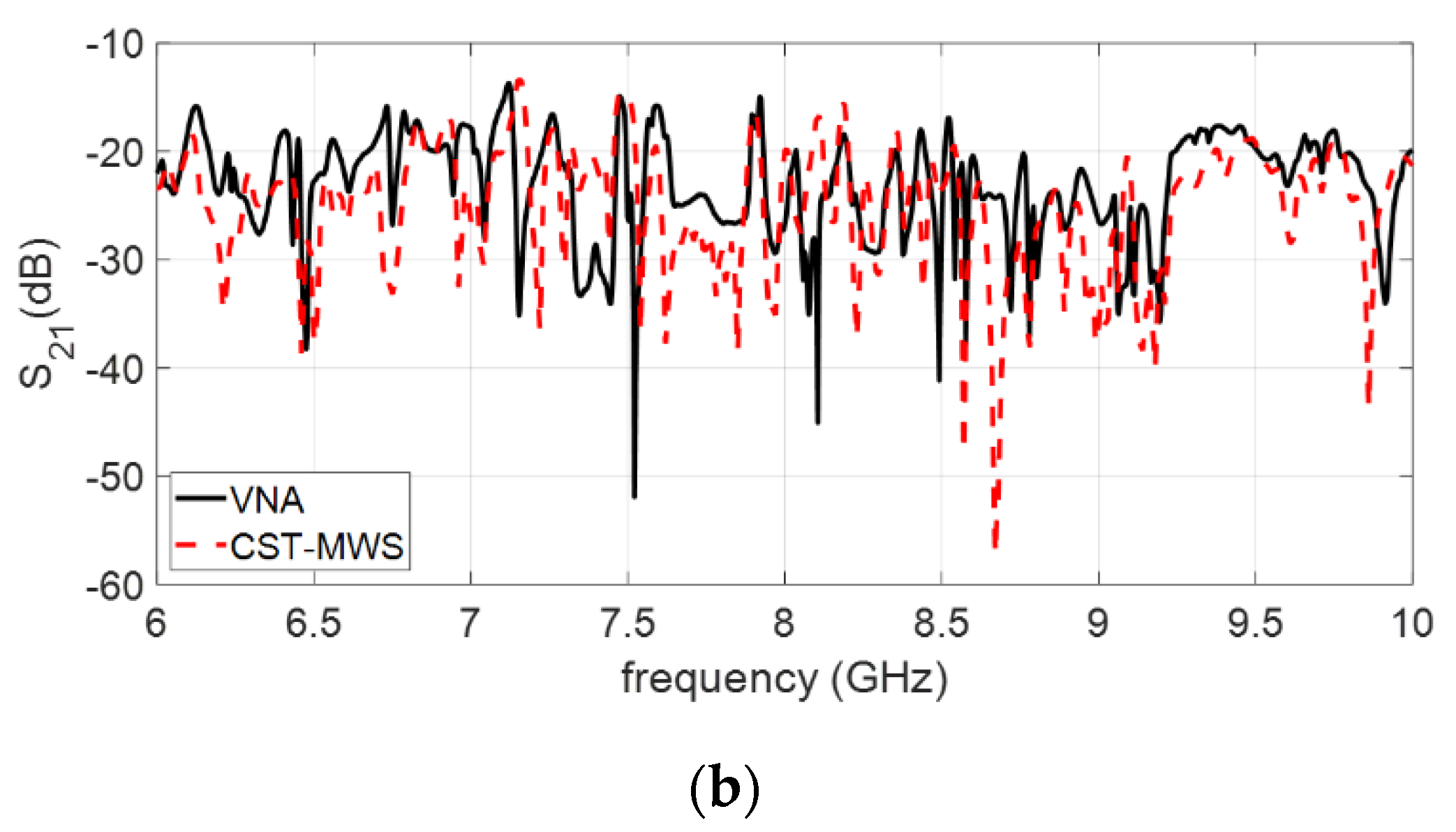
In the experimental case, the forward step is performed experimentally using a VNA. To conduct this, the scattering parameter between the two monopole antennas (representing the source and the sensor) is recorded in the frequency domain. Figure 6 shows the measured scattering parameter S21 associated with the experimental setup shown in Figure 3. The calibration routine for the VNA was performed from the end of the cables shown in Figure 3b, so that the connectors used to build the two monopole antennas do not affect the calibration. The scattering parameter S21, obtained by way of the CST MWS software, is also shown in Figure 6. In Figure 6, the frequency range of the measurement is divided into two parts, from 0 to 6 GHz (Figure 6a) and from 6 to 10 GHz (Figure 6b).
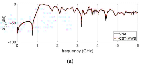
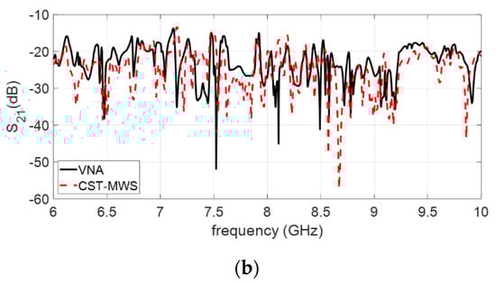
Figure 6.
The scattering parameter obtained using the VNA and the full-wave CST MWS software. (a) The scattering parameter in the 0–6 GHz range. (b) The scattering parameter in the 6–10 GHz range.
As seen in Figure 6a, there is an excellent agreement in the 0–6 GHz frequency range between the CST MWS simulations and the experimental data. For frequencies beyond 6 GHz, the agreement between the measured and simulated results deteriorates, essentially because of the effect of the antenna connectors and mismatches between the numerical model and the experimental setup.
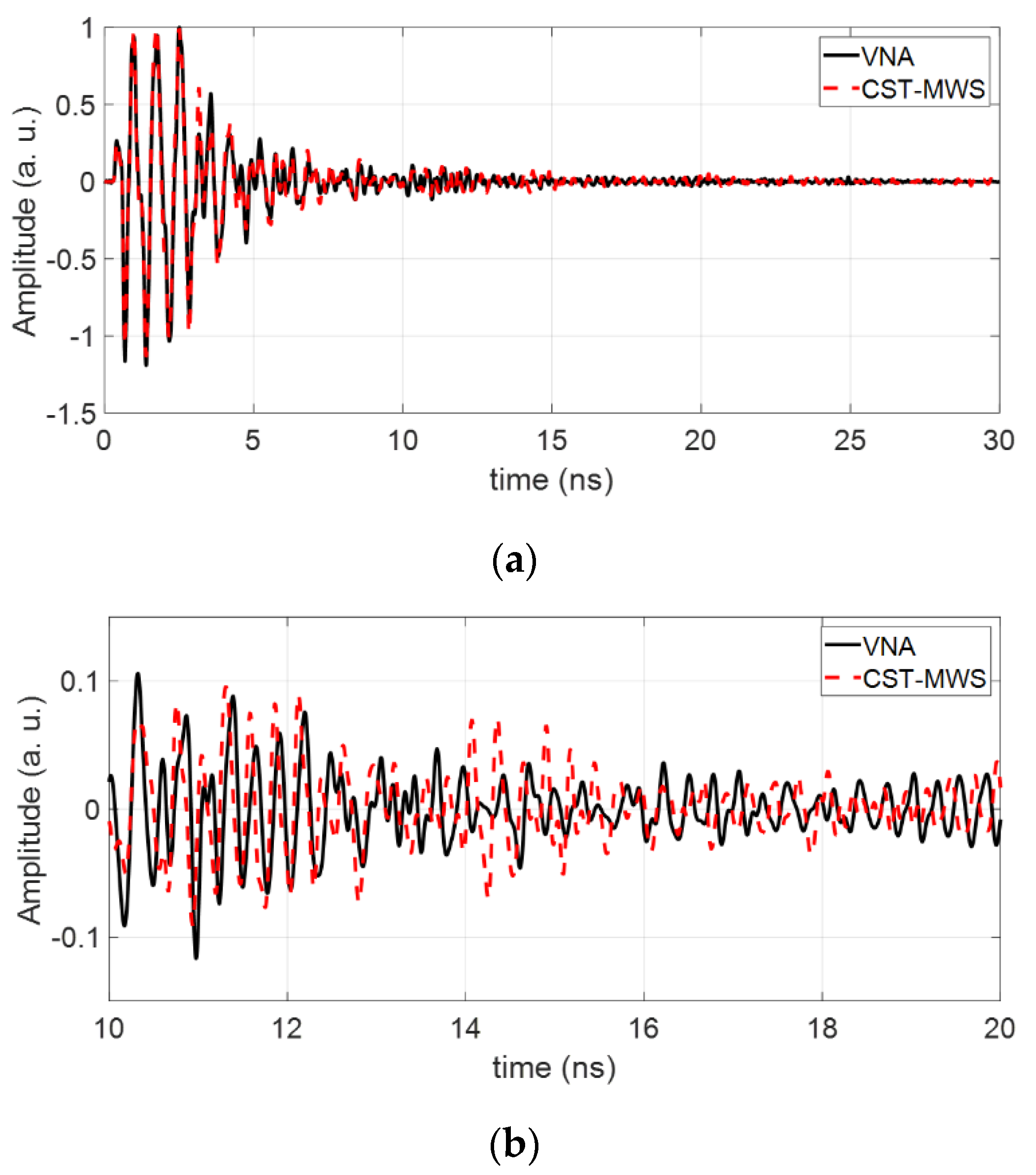
The time domain signal captured by the sensor can be obtained by multiplying the spectrum of the Gaussian pulse shown in Figure 2 by the scattering parameter S21 and applying the inverse fast Fourier transform. The result is depicted in Figure 7. The results obtained using CST MWS are also shown in that figure. It can be seen that the numerical simulations are in very good agreement with the experimental data (measured by the VNA), especially in the early times.

Figure 7.
Time-domain sensor signal obtained by way of the frequency domain measurement of the scattering parameter S21 using the VNA (black solid curve) and the full-wave CST MWS software (red, dashed line) (a) in the 030 ns time interval and (b) in the 1020 ns interval.
3.3. Experimental Validation
According to the EMTR technique, the sensor signal is time reversed and back injected into the model of the structure, which we modeled in the CST MWS environment. In this step, we consider two case studies. In the first case study, the numerical model used for the medium in the backward step is identical to the one in the forward model (matched media). It should be noted that in practical EMC problems, the location of the source(s) is unknown.
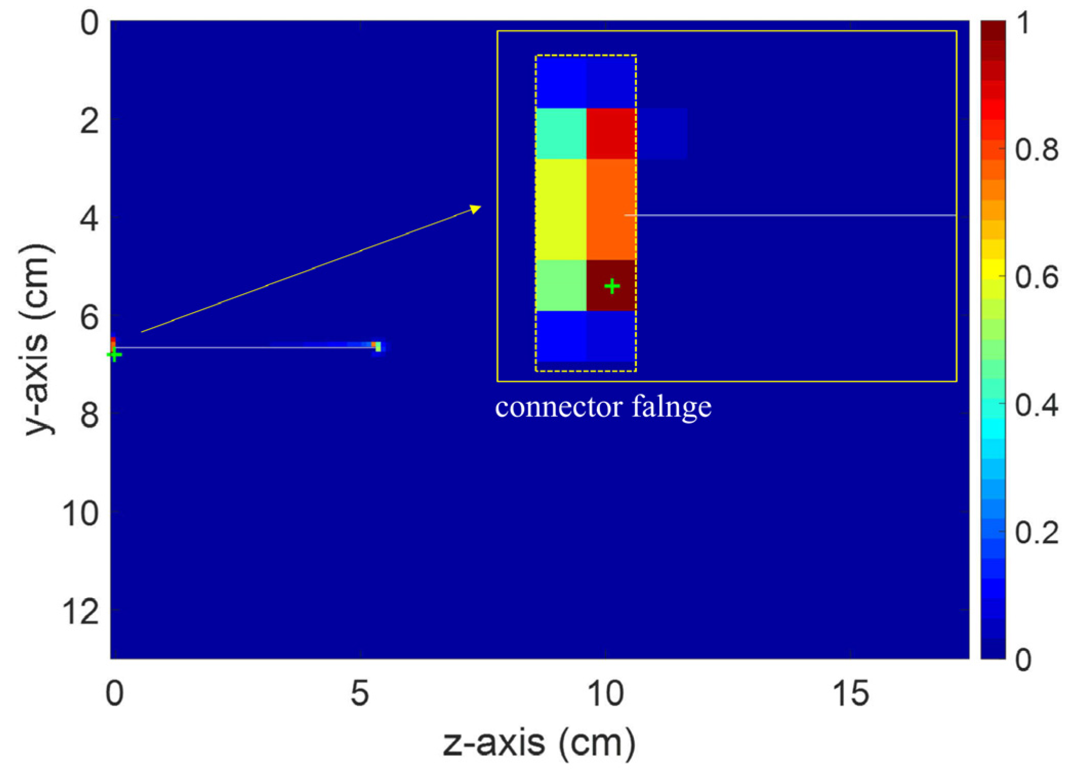
Figure 8 shows the distribution of the maximum normalized power for cut plane x = 14.78 cm in the matched-media case study. It can be seen that the maximum power occurs around the connector flange (that is, the feed point of the monopole antenna). A local maximum also occurs at the tip of the monopole antenna. The inset figure shows a zoomed view around the connector flange, where the global maximum power occurred. As can be seen from Figure 8, the EMTR method can localize the feed point of the antenna with high accuracy.
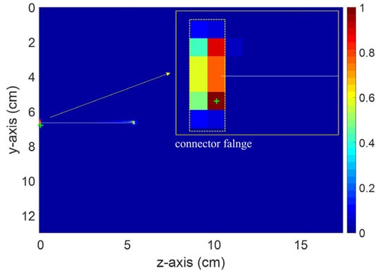
Figure 8.
Distribution of the normalized maximum power over the calculation domain in presence of the source monopole antenna (matched media) at cut plane x = 14.78 cm. The solid white line represents the location of the source monopole antenna.
In the second case study, the source monopole antenna was removed from the model shown in Figure 1 in the backward propagation step. Since the length of the antenna is 5.3 cm, which is significant compared to the dimensions of the open cavity (more than 20% of the longest dimension), removing it introduces a mismatch between the media in the forward and backward steps that can, in principle, affect the performance of the EMTR technique. Note that the classical applications of time reversal require that the backward-propagation medium be identical to the one in the forward propagation step (the so-called matched-media condition). The choice of removing the source antenna was based on our effort to consider a realistic scenario to a real EMC problem. In such a problem, the location of the source is unknown and the aim of this method is to perform source localization. Hence, in the backward propagation step, the source antenna was removed. This scenario is known as time reversal in mismatched media (e.g., [11,29]). It has been shown (e.g., [30]) that for a moderate lumped mismatch between the forward- and backward-propagation media, the focusing property of time reversal remains intact.
The distribution of the normalized maximum power over the computational domain and over the whole time for cut planes perpendicular to the x and to the y axes are depicted in Figure 9 and Figure 10, respectively. In both figures, the white line represents the location of the (removed) transmitter monopole antenna as shown in Figure 4. As can be seen, the maximum power criterion can be used to estimate the location of the EMI source with a suitable mask window.
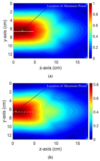
Figure 9.
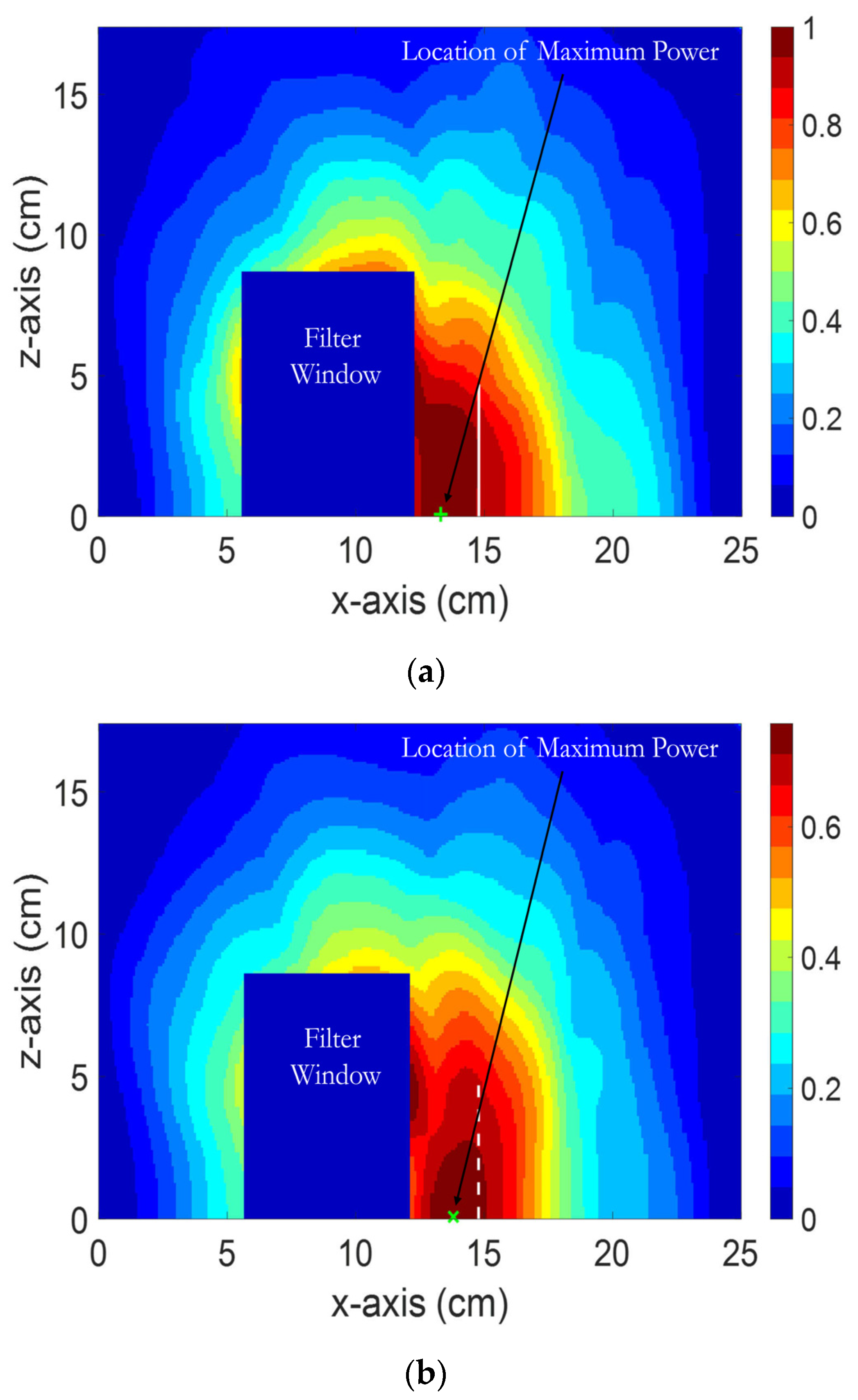
Distribution of the normalized maximum power over the calculation domain in absence of the source monopole antenna (mismatched media): (a) At cut plane x = 14.78 cm. The solid white line represents the location of the removed source monopole antenna. (b) At cut plane x = 16.78 cm. The white dashed line represents the projection of the removed source monopole antenna on the cut plane. The location of maximum power is shown using a green “+” sign.
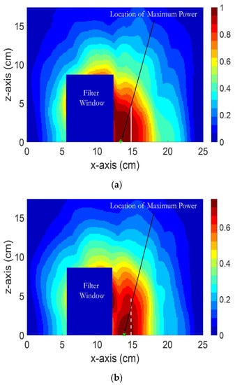
Figure 10.
Distribution of the normalized maximum power over the calculation domain in absence of the source monopole antenna (mismatched media): (a) At cut plane y = 6.66 cm. The solid white line represents the location of the removed source monopole antenna. (b) At cut plane y = 8.66 cm. The white dashed line represents the projection of the removed source monopole antenna on the cut plane. The location of maximum power is shown using a green “+” sign.
In Figure 9a,b, the distribution of the maximum power is shown for cut planes x = 14.78 cm (coincident with the x–z plane where the monopole source antenna is located) and x = 16.78 cm, 2 cm (2λ/3 at the maximum frequency of the excitation bandwidth), respectively, away from the monopole source antenna plane. It can be seen in Figure 9a,b that the maximum power of the back-propagated wave decreases as the distance from the source increases.
In Figure 10a,b, the distribution of the maximum power is shown at cut planes y = 6.66 cm (coincident with the x–z plane where the monopole source antenna is located) and y = 8.74 cm, 2 cm (2λ/3 at the maximum frequency of the excitation bandwidth) away from the monopole source antenna plane, respectively. In these cut planes, a 6.5 × 8.5 cm2 mask was used to remove the effect of the enhancement of the power near the sensor.
It should be noted that the global maximum power is located at (x = 13.3 cm, y = 6.5 cm, and z = 0.75 cm). If we assumed the location of the source to be the feed point of the monopole antenna at (x = 14.78 cm, y = 6.66 cm, and z = 0.0 cm), the three-dimensional location error in the experimental validation is 1.49 cm. The location error can be further reduced by improving the numerical model of the cavity structure.
The results of the distribution of the maximum power in Figure 9 and Figure 10 clearly show an intensification around the position of the antenna. The presented case studies suggest that EMTR can also be envisaged as a means to locate sources that are not point-like and extend over a certain volume. However, more in-depth investigations are needed before EMTR can be applied to extended sources.
4. Conclusions
The localization of electromagnetic interference (EMI) sources is one of the main challenges in electromagnetic compatibility applications. Recently, a novel approach based on the concept of time-reversal cavity was proposed to localize EMI sources, and it was validated numerically. In realistic scenarios, the signal in the forward step is obtained experimentally, while the backward step needs to be performed through numerical simulations.
In this paper, we presented, for the first time, an experimental validation of the time-reversal procedure to locate EMI sources in which the forward step signals are measured in an experimental setup and the backward step is implemented through a software simulation.
The considered experimental setup comprised a partially open cavity as the medium and two monopole antennas to emulate the EMI source and the sensor (receiving antenna), respectively. Assuming that the location of the source is the feed point of the monopole antenna, the resulting three-dimensional location error was only 1.49 cm, which is about one-third of the length of the monopole antenna, corresponding to about min/2 The obtained results suggest that EMTR can also be envisaged to locate sources that are not point-like and that extend over a certain volume. Further investigations are ongoing on the effect of the size of the antenna, the choice of the EMI source waveshape, and the distance to the source from the sensor.
Author Contributions
Conceptualization, H.K., M.A., Z.W., M.R. and F.R.; methodology, H.K., M.A. and Z.W.; software, H.K.; validation, H.K., M.A. and Z.W.; resources, F.R. and M.R.; writing—original draft preparation, H.K.; writing—review and editing, H.K., M.A., Z.W., M.R. and F.R.; supervision, M.R. and F.R. All authors have read and agreed to the published version of the manuscript.
Funding
This work was partially funded by the EPFL ENABLE Program.
Institutional Review Board Statement
Not applicable.
Informed Consent Statement
Not applicable.
Data Availability Statement
The data that support the findings of this study are available upon reasonable request from the corresponding author.
Conflicts of Interest
The authors declare no conflict of interest.
References
- Zaridze, R.; Tabatadze, V.; Petoev, I.; Kakulia, D.; Tchabukiani, T. Emission source localization using the method of auxiliary sources. In Proceedings of the IEEE International Symposium on Electromagnetic Compatibility, Wroclaw, Poland, 5–9 September 2016; pp. 829–834. [Google Scholar]
- Hao, X.C.; Xie, S.G.; Zeng, X.Y.; Du, X.; Wang, C. A near-field radiation source localization method based on passive synthetic arrays using single channel receiver. In Proceedings of the 2015 IEEE 6th International Symposium on Microwave, Antenna, Propagation, and EMC Technologies (MAPE), Shanghai, China, 28–30 October 2015; pp. 31–35. [Google Scholar]
- Kuznetsov, Y.; Baev, A.; Gorbunova, A.; Konovalyuk, M.; Thomas, D.; Smartt, C.; Baharuddin, M.H.; Russer, J.A.; Russer, P. Localization of the equivalent sources on the PCB surface by using ultra-wideband time domain near-field measurements. In Proceedings of the IEEE International Symposium on Electromagnetic Compatibility, Wroclaw, Poland, 5–9 September 2016; pp. 1–6. [Google Scholar]
- Maheshwari, P.; Kajbaf, H.; Khilkevich, V.V.; Pommerenke, D. Emission Source Microscopy Technique for EMI Source Localization. IEEE Trans. Electromagn. Compat. 2016, 58, 729–737. [Google Scholar] [CrossRef]
- Rachidi, F.; Rubinstein, M.; Paolone, M. Electromagnetic Time Reversal: Application to EMC and Power Systems; Wiley: New York, NY, USA, 2017. [Google Scholar]
- El-Sallabi, H.; Kyritsi, P.; Paulraj, A.; Papanicolaou, G. Experimental Investigation on Time Reversal Precoding for Space–Time Focusing in Wireless Communications. IEEE Trans. Instrum. Meas. 2010, 59, 1537–1543. [Google Scholar] [CrossRef]
- Lerosey, G.; De Rosny, J.; Tourin, A.; Derode, A.; Fink, M. Time reversal of wideband microwaves. Appl. Phys. Lett. 2006, 88, 154101. [Google Scholar] [CrossRef]
- Lerosey, G.; De Rosny, J.; Tourin, A.; Derode, A.; Montaldo, G.; Fink, M. Time Reversal of Electromagnetic Waves. Phys. Rev. Lett. 2004, 92, 193904. [Google Scholar] [CrossRef]
- Wu, B.; Gao, Y.; Laviada, J.; Ghasr, M.T.; Zoughi, R. Time-Reversal SAR Imaging for Nondestructive Testing of Circular and Cylindrical Multilayered Dielectric Structures. IEEE Trans. Instrum. Meas. 2019, 69, 2057–2066. [Google Scholar] [CrossRef] [Green Version]
- Wang, Q.; Xu, Y.; Su, Z.; Cao, M.; Yue, N. An Enhanced Time-Reversal Imaging Algorithm-Driven Sparse Linear Array for Progressive and Quantitative Monitoring of Cracks. IEEE Trans. Instrum. Meas. 2018, 68, 3433–3445. [Google Scholar] [CrossRef]
- Liu, D.; Vasudevan, S.; Krolik, J.; Bal, G.; Carin, L. Electromagnetic Time-Reversal Source Localization in Changing Media: Experiment and Analysis. IEEE Trans. Antennas Propag. 2007, 55, 344–354. [Google Scholar] [CrossRef] [Green Version]
- Mora, N.; Rachidi, F.; Rubinstein, M. Application of the time reversal of electromagnetic fields to locate lightning discharges. Atmos. Res. 2012, 117, 78–85. [Google Scholar] [CrossRef]
- Karami, H.; Azadifar, M.; Mostajabi, A.; Rubinstein, M.; Rachidi, F. Numerical and Experimental Validation of Electromagnetic Time Reversal for Geolocation of Lightning Strikes. IEEE Trans. Electromagn. Compat. 2020, 62, 2156–2163. [Google Scholar] [CrossRef]
- Karami, H.; Azadifar, M.; Mostajabi, A.; Favrat, P.; Rubinstein, M.; Rachidi, F. Localization of Electromagnetic Interference Sources Using a Time-Reversal Cavity. IEEE Trans. Ind. Electron. 2021, 68, 654–662. [Google Scholar] [CrossRef]
- Wang, Z.; Rachidi, F.; Paolone, M.; Rubinstein, M.; Razzaghi, R. A Closed Time-Reversal Cavity for Electromagnetic Waves in Transmission Line Networks. IEEE Trans. Antennas Propag. 2021, 69, 1621–1630. [Google Scholar] [CrossRef]
- Lugrin, G.; Parra, N.M.; Rachidi, F.; Rubinstein, M.; Diendorfer, G. On the Location of Lightning Discharges Using Time Reversal of Electromagnetic Fields. IEEE Trans. Electromagn. Compat. 2014, 56, 149–158. [Google Scholar] [CrossRef]
- Nobrega, L.A.M.M.; Costa, E.G.; Serres, A.J.R.; Xavier, G.V.R.; Aquino, M.V.D. UHF Partial Discharge Location in Power Transformers via Solution of the Maxwell Equations in a Computational Environment. Sensors 2019, 19, 3435. [Google Scholar] [CrossRef] [PubMed] [Green Version]
- Karami, H.; Rachidi, F.; Rubinstein, M. On Practical Implementation of Electromagnetic Time Reversal to Locate Lightning. In Proceedings of the 23rd International Lightning Detection Conference (ILDC), Tucson, AZ, USA, 18–21 March 2014. [Google Scholar]
- Karami, H.; Rachidi, F.; Rubinstein, M. On the use of Electromagnetic Time Reversal for lightning location. In Proceedings of the 2015 1st URSI Atlantic Radio Science Conference (URSI AT-RASC), Gran Canaria, Spain, 16–24 May 2015. [Google Scholar]
- Wang, T.; Qiu, S.; Shi, L.-H.; Li, Y. Broadband VHF Localization of Lightning Radiation Sources by EMTR. IEEE Trans. Electromagn. Compat. 2017, 59, 1949–1957. [Google Scholar] [CrossRef]
- Wang, T.; Shi, L.-H.; Qiu, S.; Sun, Z.; Zhang, Q.; Duan, Y.-T.; Liu, B. Multiple-Antennae Observation and EMTR Processing of Lightning VHF Radiations. IEEE Access 2018, 6, 26558–26566. [Google Scholar] [CrossRef]
- Liu, B.; Shi, L.-H.; Qiu, S.; Liu, H.-Y.; Sun, Z.; Guo, Y.-F. Three-Dimensional Lightning Positioning in Low-Frequency Band Using Time Reversal in Frequency Domain. IEEE Trans. Electromagn. Compat. 2019, 62, 774–784. [Google Scholar] [CrossRef]
- Karami, H.; Mostajabi, A.; Azadifar, M.; Wang, Z.; Rubinstein, M.; Rachidi, F. Locating Lightning Using Electromagnetic Time Reversal: Application of the Minimum Entropy Criterion. In Proceedings of the International Symposium on Lightning Protection (XV SIPDA), Sao Paulo, Brazil, 30 September–4 October 2019. [Google Scholar]
- Karami, H.; Azadifar, M.; Rubinstein, M.; Karami, H.; Gharehpetian, G.B.; Rachidi, F. Partial Discharge Localization Using Time Reversal: Application to Power Transformers. Sensors 2020, 20, 1419. [Google Scholar] [CrossRef] [PubMed] [Green Version]
- Azadifar, M.; Karami, H.; Wang, Z.; Rubinstein, M.; Rachidi, F.; Karami, H.; Ghasemi, A.; Gharehpetian, G.B. Partial Discharge Localization Using Electromagnetic Time Reversal: A Performance Analysis. IEEE Access 2020, 8, 147507–147515. [Google Scholar] [CrossRef]
- Karami, H.; Azadifar, M.; Rubinstein, M.; Rachidi, F. An experimental validation of partial discharge localization using electromagnetic time reversal. Sci. Rep. 2021, 11, 1–12. [Google Scholar] [CrossRef] [PubMed]
- Karami, H.; Azadifar, M.; Mostajabi, A.; Rubinstein, M.; Rachidi, F. Localization of Electromagnetic Interference Source Using a Time Reversal Cavity: Application of the Maximum Power Criterion. In Proceedings of the IEEE International Symposium on Electromagnetic Compatibility, Signal Integrity and Power Integrity, Reno, NV, USA, 28 July–28 August 2020. [Google Scholar]
- Paul, C.R. Introduction to Electromagnetic Compatibility, 2nd ed.; Wiley: New York, NY, USA, 2006. [Google Scholar]
- Bal, G.; Ram, R.; Ver´astegui, R.; Ver´astegui, V. Time Reversal In Changing Environments. Soc. Ind. Appl. Math. 2004, 2, 639–661. [Google Scholar] [CrossRef]
- Wang, Z.; Hamidreza, K.; Parisa, D.; Seyed, S.; Hesmedin, H.; Reza, R.; Mario, P.; Marcos, R.; Farhad, R. An Experimental Study on Electromagnetic Time Reversal Focusing Property in Mismatched Media. In Proceedings of the URSI GASS, Sapienza Faculty of Engineering, Rome, Italy, 28 August–4 September 2021. [Google Scholar]


Publisher’s Note: MDPI stays neutral with regard to jurisdictional claims in published maps and institutional affiliations. |
© 2021 by the authors. Licensee MDPI, Basel, Switzerland. This article is an open access article distributed under the terms and conditions of the Creative Commons Attribution (CC BY) license (https://creativecommons.org/licenses/by/4.0/).