Abstract
This work focuses on the optimization of a last-mile delivery system with multiple transportation modes. In this scenario, parcels need to be delivered to each customer point. The major feature of the problem is the combination of a fleet of road vehicles (vans) with a drone. Each van visits a subset of demand nodes to be determined according to the route of the van. The drone serves the customers not served by vans. At the same time, considering the safety, policy and terrain as well as the need to replace the battery, the drone needs to be transported by truck to the identified station along with the parcel. From each such station, the drone serves a subset of customers according to a direct assignment pattern, i.e., every time the drone is launched, it serves one demand node and returns to the station to collect another parcel. Similarly, the truck is used to transport the drone and cargo between stations. This is somewhat different from the research of other scholars. In terms of the joint distribution of the drone and road vehicle, most scholars will choose the combination of two transportation tools, while we use three. The drone and vans are responsible for distribution services, and the trucks are responsible for transporting the goods and drone to the station. The goal is to optimize the total delivery cost which includes the transportation costs for the vans and the delivery cost for the drone. A fixed cost is also considered for each drone parking site corresponding to the cost of positioning the drone and using the drone station. A discrete optimization model is presented for the problem in addition to a two-phase heuristic algorithm. The results of a series of computational tests performed to assess the applicability of the model and the efficiency of the heuristic are reported. The results obtained show that nearly 10% of the cost can be saved by combining the traditional delivery mode with the use of a drone and drone stations.
1. Introduction
The study of operations research models and methods for problems involving unmanned aerial vehicles (UAVs) has become quite popular in the second decade of the 2000 s. In addition to applications in last-mile delivery operations as we are considering in this paper, we also find applications related to military operations (e.g., surveillance), environmental protection (e.g., fire prevention), agriculture (monitoring of large areas considering factors such as slope and elevation), emergency logistics (pre-screening of damaged areas and roads), etc.
In logistics distribution, the use of drones has become pervasive. The benefits of using UAVs for parcel delivery are nowadays clear: (i) drones are faster and incur lower unit costs; (ii) drones do not require manual operation; (iii) UAVs are not subject to terrain and traffic conditions; (iv) there are many environmental benefits associated with the use of UAVs (as can be seen, e.g., in Figliozzi 2017 and Goodchild and Toy 2018) [1,2]. It is important to note, however, that there are also some shortcomings related to this delivery mode: (i) the carrying capacity of drones is limited—the load capacity of ordinary rotor drones usually does not exceed 50 kg; and (ii) for safety reasons, drones can usually only carry one piece of cargo at a time, and the short driving radius of drones requires frequent trips between customer points and warehouses/distribution centers.
On the other hand, traditional delivery modes (e.g., by road) can satisfy several customers using a single route. Moreover, the capacity of a vehicle is of course greater than that of drones. Overall, this mode can benefit from economies of scale although the distribution cost may be higher. A strong disadvantage is that road transportation is susceptible to traffic conditions and terrain obstacles.
The above considerations make it clear that by combining the two above transportation modes, we can simultaneously take advantage and circumvent the disadvantages of both. Furthermore, we recently observed technological developments motivating the study of problems such as the one we are considering: the industry has conceived vehicles that can carry a drone and act as drone dock-stations to thus position a drone in a more convenient location for supplying a set of delivery orders. This is the case with the new ”vans and drones” concept launched by Mercedes-Benz in which the roof of a van is used as a landing platform for drones (https://www.mercedes-benz.com/en/vehicles/transporter/vans-drones-in-zurich/, accessed on 1 March 2020).
In this paper, we investigated a multi-mode multiple traveling salesman problem motivated by applications in the context of last-mile distribution. We consider the situation in which a classical transportation mode (e.g., a fleet of road vehicles (vans)) is combined with an alternative that has recently emerged as very competitive under certain circumstances, i.e., in this case, the use of an unmanned aerial vehicle (UAV), known more popularly as a drone.
In many cases, the distance between the demand nodes and the depot prevents the use of drones. When a drone is used for distribution, the demand point is often in the suburbs far away from urban areas. For example, during distribution in some mountainous villages, drones may face undertaking operations such as flying around a mountain, so it would be safer for the drone to take off from a local station and return to the station after distribution. Thus, another possibility is to position a drone in previously authorized sites—hereafter called drone stations—from where its use once again becomes a possibility. This course of action can be accomplished using a special vehicle (truck) that carries the drone as well as the parcels that it will deliver. At the same time, trucks can also travel between stations with the drone and parcels. Therefore, it is more reasonable to set up a drone station and deploy drones from the station rather than a moving truck. The drone can also charge at the station.
Direct assignment is assumed for the demand nodes served by the drone, i.e., the drone visits one demand node each time it returns to the station to collect the parcel in the truck for another demand node (before eventually returning for recharging). When all demand nodes assigned to a drone station are served, the truck may position the drone in another drone station or stay in the station.
In this work, we neglect the capacity of the vehicles and we assume that a unique parcel is to be delivered to each demand node. Hence, the problem we are investigating consists of combining a multiple traveling salesman problem (for the fleet of road-delivery vehicles) with a location-allocation problem (for the drone pre-positioning and delivery). The need for previously identifying potential drone stations is motivated by safety regulations in many countries (e.g., the Federal Aviation Administration (FAA) in the USA) that prevent drones from being launched from moving vehicles.
The decisions to make in our problem comprise (i) the drone stations to visit by the drone-carrying vehicle; (ii) the assignment of demand nodes to drone stations; and (iii) the routes for serving the demand nodes that will be served by vans. The goal is to minimize the total transportation cost and a fixed cost of using the drone stations.
In Figure 1, we illustrate the problem. In this area, D represents the distribution center, and the star polygons such as and represent the used drone stations. The dots such as a and b represent demand nodes. After receiving the order, the vans depart from the distribution center to serve a given customer point. For example, the route of one of the vans is . At the same time, the truck transporting a drone also departs from the distribution center and first arrives at station . After arriving at station , the truck stays at station and the drone is deployed from the truck. The drone will return to the truck at station after serving demand node a, and then deliver to service points b and c. After the drone has completed all its tasks (serving demand nodes a, b and c) and returned to the truck, the truck transports the drone to station for the next stage of service, and finally returns to the depot.
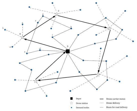
Figure 1.
Illustrative example for the mTSP-LAP solution.
In Figure 1, we can also observe that the problem cannot be separated according to the transportation modes since the one decision that needs to be taken concerns the mode to use for satisfying each demand node. It is also worth noting that typically a drone does not perform along a route. Instead, the drone picks up the package from the truck parked at the station and serves the customer point. Summing up, the problem we are investigating is a multi-mode multiple traveling salesman problem intertwined with a location-allocation problem, which we abbreviate to mTSP-LAP.
In this paper, we refer to this distribution method to establish a mathematical model about mTSP-LAP and designed a heuristic algorithm to solve it. Finally, we generated an area and some customer points, verified the effectiveness of our proposed model and algorithm through numerical experiments and performed a sensitivity analysis. The main contributions of this paper include: (1) a new logistics distribution model in which using a drone is proposed and a numerical analysis shows that this distribution model is more efficient in cost; (2) for this distribution model, we propose an integer programming model called mTSP-LAP (multiple traveling salesman problem intertwined with a location-allocation problem); (3) for the mTSP-LAP model, we designed a two-stage heuristic algorithm to solve it.
The remainder of this paper is organized as follows. In Section 2, we review the literature related to our work. In Section 3, we discuss an integer optimization model for the problem. The following section—Section 4—is devoted a heuristic algorithm for the problem. The results of the computational tests performed using the mathematical model and the heuristic algorithm are reported in Section 5. The paper ends with an overview of the work achieved herein.
2. Relation with the Existing Literature
In this part, we summarize the traveling salesman problem (TSP) and the application of drone in the logistics field. As a classic traditional problem, TSP has been a hot topic in the field of logistics in the last ten years. In terms of research on drones, the use of drones in distribution has been some paid attention to a certain extent, and the vehicle routing problem of joint distribution between the drone and van is the focus of our research.
2.1. TSP and MTSP
The traveling salesman problem (TSP) is one of the most studied combinatorial optimization problems [3,4]. Nevertheless, the problem is still attracting the attention of the scientific community which is pursuit of the development of progressively more competitive algorithms to solve it. Nagata and Kobayashi (2013) enhanced the use of genetic algorithms using a so-called edge assembly crossover (EAX) [5]. A local search procedure in EAX is used to determine good combinations of building blocks of parent solutions for generating even better offspring solutions from very high-quality parent solutions. More recently, Ozden et al. (2017) described and compared serial, parallel and distributed solver implementations for large batches of traveling salesman problems using the Lin–Kernighan heuristic (LKH) and the Concorde solver [6,7]. Finally, we quote the work of Staněk et al. (2019) who investigated two variants of the Euclidean TSP based on so-called turning angles [8]. The authors proposed several heuristics based on the geometric properties of the optimal solution as well as on LP relaxations.
New variants and extensions of the TSP also keep being considered, motivated by real-world problems. Some recent ones include that of Coutinho et al. (2016), who addressed the so-called close-enough TSP [9]. In this problem, rather than visiting a node (customer), the salesman must visit a specific region containing such a node. This problem was further analyzed by Wang et al. (2019) who proposed new a competitive heuristic for it [10]. Carlsson et al. (2018) considered a distributionally robust Euclidean TSP that consists of finding the worst-case spatial distribution of demand against all distributions [11]. The Wasserstein distance was also considered [12]. Montero et al. (2017) investigated a TSP with time windows [13]. Malaguti et al. (2018) investigated a pickup and delivery TSP in the context of maritime transportation [14]. In this problem, each customer has a demand characterized by a weight. The pickups and deliveries are performed by a single ship of given weight capacity. The ship is able to visit a port only if the amount of cargo it carries is compatible with the draft limit of the port. Errico et al. (2017) presented the symmetric TSP with generalized latency [15]. The underlying idea is to consider an objective function that in addition to the usual cost also accounts for the travel times of passengers in a transit system. Gupta et al. (2017) investigated a so-called adaptive TSP: considering a metric space, the set of nodes that required visiting is not known in advance; one only knows that upon arriving at a node [16].
In the current paper, we consider a multiple TSP (mTSP) which is the extension of the TSP in which we have multiple salesman based upon one or several depots [17]. In such a context and considering some recent works, we quote the paper by Zhou et al. (2018) that presents two partheno-genetic algorithms (PGA) for the problem [18]. These were compared with a particle swarm optimization algorithm (PSO) and a so-called invasive weed optimization algorithm. Soylu (2015) considered two objective functions separately for the mTSP: the longest tour length (to minimize); and the total length of all tours [19]. A general variable neighborhood search was proposed. Xu and Rodrigues (2017) extended the well-known Christofides heuristic which is an improvement on the two current best approximation algorithms [20,21]. Bektaş (2012) proposed Benders decomposition algorithms based upon new formulations for a new extension of the problem: a range is assumed for the number of demand nodes that each salesman should visit [22]. Kota and Jarmai (2015) introduced an algorithm for the fixed destination multi-depot mTSP with multiple tours [23]. Dhein et al. (2018) considered a variant of the mTSP in which the distance between any two salesmen cannot be greater than a pre-specified value to ensure that the salesman can assist each other in a timely manner if an emergency occurs [24].
We can also find literature focusing on the multi-mode mTSP. Gambella et al. (2018) considered two transportation modes and investigated a 2TSP [25]. The authors assumed a slow carrier with a long operational range and a faster vehicle (e.g., UAV) with a limited operational range. The carrier follows a route and delivers parcels to some customers. For some other customers, the UAV is launched to perform the delivery. An exact algorithm was proposed for the problem. This same problem was also investigated by Erdoğan and Yldrm (2021), who explored new properties of the problem, proposing a mixed-integer second-order conic optimization formulation together with an iterated local search algorithm [26].
2.2. Delivery by Drone
The rapid development and pervasive use of UAVs together with the continuous growth of e-commerce significantly increased the relevance of this transportation mode in logistics and distribution systems [27,28]. Murray and Chu (2015) performed one of the first works investigating the use of drone-carrying vehicles in transportation systems [29]. The problem is called the flying sidekick traveling salesman problem (FSTSP). A set of demand nodes is considered that are to be served either directly by the truck or by the UAV operated in coordination with the carrier. Carlsson and Song (2018) considered a UAV–truck system assuming that the UAV provides a service to customers while making return trips to the truck that keeps moving [30]. Agatz et al. (2018) proposed an exact algorithm for this same problem, calling it a TSP with drone (TSP-D) [31]. Yurek and Ozmutlu (2018) presented an iterative algorithm that is based on a decomposition approach to minimize delivery completion time for the same TSP-D [32]. Ha et al. (2018) considered a new variant of the TSP-D in which the objective is to minimize operational costs that include the total transportation cost as well as the cost associated with the wasted time during which a vehicle has to wait for another [33]. Pina-Pardo et al. (2021) introduced the so-called TSP with release dates and drone resupply [34]. This is a problem consisting of finding a minimum time route for a single truck that can receive newly available orders en route via a drone sent from the depot. These authors assumed that the orders’ release dates are known at the time of delivery planning.
Kitjacharoenchai et al. (2019) considered a multiple truck–drone system based upon a single depot [35]. In this case, the drones fly from delivery trucks, making the assigned deliveries and returning to any available truck nearby. The objective is to minimize the arrival time of all trucks and drones to the depot after completing the deliveries. Ham (2018) extended this problem by considering multiple depots, time windows as well as pickup and delivery operations [36]. One important feature that has also been considered in the literature concerns the autonomy of UAVs. Kim et al. (2018) considered an mTSP in which drones were the only type of vehicle (salesman) [37]. The authors introduced a robust optimization model for the problem that consists of defining multiple drone path deliveries considering uncertainty in the duration of the battery. Each drone is assigned to a specific depot and operates only from/to there.
In the literature focusing on the mTSP, we observe that in the large majority of cases, a single transportation mode is considered. When this is not the case, we find a carrier–vehicle TSP in which deliveries can be made by the truck or by the drone it carries. In other words, to the best of the authors’ knowledge, the setting we are investigating has not been investigated in the literature: the combination of a truck–drone vehicle and a classic fleet of vehicles. We also stress the fact that some countries still forbid the use of drones from moving vehicles which makes the use of drones for long-range distribution feasible only if the drone is previously positioned closer to the demand nodes. These aspects give relevance to our work—we go beyond the existing literature contributing to the combination of a truck–drone system and other “standard” delivery options. Our study considers adding stations for drones, first transporting some packages and drones to the stations by trucks and then using drones for distribution, thereby reducing the distance of drone distribution and increasing the probability of using drones. In addition, we developed a two-stage heuristic algorithm to arrive at a more reasonable distribution plan in a reasonably short time.
3. Mathematical Model
We recall the decisions we consider in our mTSP-LAP: (i) the delivery mode used to serve each demand node (by road as part of a route or by air directly by the drone); (ii) the routes for road delivery; (iii) the stations used to park the truck as well as release and recover the drone; and (iv) the demand nodes to be served from each drone station. We need to consider how the demand points are served, whether they are served by drone or vans, and also determine the departure and return station of the drone. These drone and vans paths also affect each other. We consider the following additional assumptions:
- All vehicles are uncapacitated—each vehicle can carry all the parcels destined to the demand nodes in the route defined for the vehicle. If the capacities of the drone and vans were considered, one can add a coefficient to the cost or add constraints on vehicle cost. This will not have a substantial impact on this mode, so this paper ignores the impact of vehicle load.
- Every customer can be supplied by the drone. If some demand points can only be served by drone or van, it reduces decision making regarding the service mode and simplifies the problem.
- We assume that the drone stations already exist and thus we just need to decide those that will be used for parking the truck as well as for launching and retrieving the drone. This will be more applicable in the case of discrete point location, and it is more in line with the original intention of focusing on path planning in this paper.
- Although the drone needs to be charged when its remaining autonomy prevents further deliveries, we ignore this aspect—namely the charging time; we exclusively focused on the transportation costs as well as the costs of using drone stations. Because our cost mainly considers the travel time, if we consider the charging time, we only need to add a fixed cost, so we choose to ignore this cost in the model.
- We ignore road congestion for road transportation and thus we assume fixed driving times for all road vehicles.
- We do not consider any obstacles when using the drone. These two hypotheses are because the problems of road congestion and airspace obstacles generally belong to the research scope of artificial intelligence science and do not belong to the field of operations research. Therefore, we do not consider these problems.
We consider a connected network G = (,) underlying the problem. In , node 0 represents the depot and N represents the set of demand nodes. A denotes the set of arcs in the network (direct road connections). For every pair , we assume that we can compute the cost for linking those nodes by road (e.g., based upon the shortest path between i and j and the per-unit distance transportation cost).
The following parameters defining our problem are considered:
| m, | number of vehicles for road delivery (vans); |
| d, | number of drone stations; |
| p, | maximum number of drone stations allowed; |
| f, | fixed cost of using the drone station; |
| , | traveling cost between nodes i and j (); |
| , | transportation cost for satisfying node i by the drone from station k (, ). |
The problem can be mathematically formulated using the following sets of decision variables:
We can finally present the following integer programing model for the mTSP-LAP:
The objective function (1) represents the total cost that includes (i) the cost of using drone stations; (ii) the transportation costs for the road delivery vehicles as well as for the drone-carrying truck; and (iii) the drone delivery cost. Because the construction of the station is a one-time cost, once the station is set up, its subsequent use, maintenance and other costs can be ignored. Therefore, we consider designing a fixed cost for the station. Constraint (2) represents the maximum number of drone stations allowed. Inequality (3) states that if a drone serves a demand node from one station then the station should be operating. Constraint (4) ensures that every demand node is served by exactly one and only one transportation mode (either by van or by drone). Constraint (5)–(6) means that it is only served by the van at both point i and point j, and there will be a path of van from i to j. Constraints (7)–(8) indicate that a total of m vans depart from the distribution center and return to the distribution center. Constraint (9) is an MTZ constraint, which ensures that there will be no sub-tours in the path of the vans [17]. Constraints (3)–(6) ensure the synchronization of the vans’ path planning with drone station selection and drone path planning. When planning the path of the vans, it is necessary to prevent the demand point being served by drone. When making drone distribution decisions, it is also necessary to prevent the demand points being served by vans. Finally, (10)–(13) define the domain of the decisions variables.
Remark 1.
The above problem contains a TSP as a particular case and thus it is NP-hard.
Remark 2.
We can relax the integrality constraints on the x-variables as well as the upper bound, thus simply writing that
In fact, it is easy to see that since the y-variables are integer, there is always one optimal solution such that the s-variables are also integer.
Remark 3.
In the above model, we include the fixed cost of using the drone station. However, in our algorithmic procedure to be proposed in the next section and when analyzing the results, we start by ignoring this component and use it last as part of a post-optimization analysis.
Looking at the above model, we easily identify the ”location-allocation” component, Constraints (2)–(3); the ”mTSP” component, Constraints (5)–(9); and the linking constraints, Constraints (4)–(6). The hardness of the problem together with many data-driven applications in which upon collecting the data a solution must be found in a very short time justifies the development of a heuristic algorithm for the problem. In fact, in many real-world last-mile delivery applications (e.g., food delivery), customers expect to be satisfied shortly after calling to be served and thus we cannot afford waiting too long to obtain an optimal solution to the problem. Nevertheless, in Section 5, we reported on some results obtained by solving the above model with an off-the-shelf solver.
4. Heuristic Algorithm
In this section, we develop a two-phase heuristic algorithm for the mTSP-LAP. In terms of the algorithm, in the first stage, we first generate a feasible solution which does not include the path of the drone. We use m-means clustering (K-means) to assign all customer points to the m vans for service. After that, for each van, we use the greedy algorithm to preliminarily calculate the path. In the first phase, we construct a solution for the mTSP (thus ignoring the drone). Note that the solution obtained after the first phase is already a feasible solution to the whole problem since the drone is not used. Because there is no path for the drone in this feasible solution, this is only an extreme case. In the second stage, we will change the service mode of some customer points to drone service according to the savings value. In this process, the algorithm will also calculate which station the drone takes off from and returns to. In this step, the stations used by the drone will be allocated. At the same time, the saving value is also used to iteratively update the path of the vans. In the second stage, the solution of the first phase is improved by including the LAP component of the problem: drone delivery is considered, whose benefit is assessed considering the estimated saving cost of changing the delivery mode for some demand nodes from road to air. Under the framework of neighborhood search, we innovatively designed the rules of transportation mode exchange, i.e., in the first stage, some demand points originally served by vans were replaced by drones. A very important point in exchange rules is to calculate whether there will be cost savings after changing the transportation mode. For this reason, we can look at the first phase as construction phase with the second phase as the improvement phase.
4.1. Construction Phase
The m-means clustering algorithm is a very popular clustering procedure that we put at the core of the first phase of our heuristic [38]. The algorithm is quite simple: given n data points in an Euclidean space, we select m in some way to define a first tentative set of centers. Each other point is then assigned to the closest center (with respect to the Euclidean distance). Afterwards, we calculate the centroids of each cluster obtaining a new set of m centers. Considering this new set, all the other points are reassigned to the closest center. This process proceeds until the solution does not change from one iteration to another.
This algorithm can be looked at as a local search procedure for finding feasible clusters minimizing the sum of the squared distances between each point and the centroid of the cluster it is allocated to. For deeper insights into the above optimization problem, the reader is referred to Aloise et al. (2012) [39].
Despite some well-known disadvantages of the m-means procedure (see, e.g., Gribel and Vidal 2019 [40]), we adopted this method since the purpose in this phase is to find a feasible solution to our problem whilst ignoring the matter of the drone. Hence, we believe that it does not compensate at this stage to invest too much in finding solutions that still neglect an important component of the problem. We start the procedure by randomly generating the m initial centers.
Once the demand nodes are clustered, a straightforward nearest-neighborhood computation is performed considering the depot and the nodes in each cluster to define the shortest length Hamiltonian tour for the nodes in that group [3].
4.2. Improvement Phase
Considering the solution constructed in the first phase, we denote by E a set of edges that will be analyzed in this phase to induce improvements in the solution. Initially, this set contains all the direct road links used by the solution. We denote by the current solution cost. We also define a set T containing all the demand nodes served by a road tour, which is of course equal to N when we start this improvement phase.
Our procedure iteratively attempts to remove nodes from T when a demand node is scheduled to be served by the drone. This is accomplished by selecting the edge
and (separately) computing saved cost among the total delivery cost (road and air) from servicing or with the drone (from the closest drone station to each node). We denote by the total delivery cost if is served by air (the Hamiltonian tour for the depot and cluster belongs to is also recomputed—using nearest-neighborhood computation as before). Similarly, we compute . Finally, we have the savings:
and:
Now, we distinguish three cases for deciding the course of action to take:
- Case 1: and .In this case, demand node is removed from T since it will be served by the drone (from the closest drone station).
- Case 2: and .In this case, demand node is removed from T since it will be served by the drone (from the closest drone station).
- Case 3: and .In this case, nodes and remain in the initially established road route and the corresponding edge is removed from the set of edges (E) to be analyzed.
The improvement phase just described is formally detailed in Algorithm 1. In this algorithm, denotes the cluster to which a node belongs to.
| Algorithm 1 Improvement Phase. |
|
After Algorithm 1 is executed, we find in set N the nodes that will be served by the drone (each one from the closest drone station).
5. Numerical Experiments
In this section, we report on a series of computational experiments performed to assess the model and algorithm discussed for the mTSP-LAP. We start by describing the test bed instances used and then we discuss the results.
All algorithms were run on Intel Core i5 macOS High Sierra 64-bit mode, with an operating frequency of 2.7 GHz and a memory of 8 Gb.
5.1. Test Data
To generate the demand nodes, a 20,000 × 20,000 square was considered with (−10,000, −10,000) as the lower-left corner and (10,000,10,000) as the upper-right corner.
Initially, 30 instances were generated that were divided into two sets. In the first set (instances 1–15), 50 demand points were randomly positioned in the underlying square. Four drone stations were assumed, which were positioned in the coordinates (5000,5000), (−5000,5000), (5000,−5000), (−5000,−5000). The depot was positioned in the center of the square. Figure 2 shows a schematic of this area. A fleet with five vans was assumed. The second set of instances (instances 16–30) differ from the above ones by randomly generating 100 demand nodes.
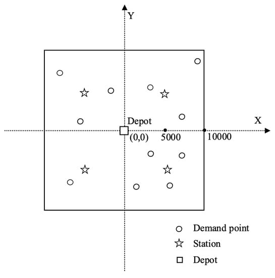
Figure 2.
Schematic diagram of test area.
We assume that the drone delivery cost is negatively correlated with the time of delivery. This is accomplished by considering that if the speed of the drone is v times that of the road vehicles, then the delivery cost of the drone for a similar distance is times that of the road vehicles. Due to the fact that the drone can fly in a straight line (which is not the case for the road vehicles which must follow the roads), we assume that the delivery distance of a road vehicle is 1.4 times that of the drone for the same straight-line distance. This is because the distance between two points generally uses Euclidean distance for drone, while road vehicles generally use Manhattan distance. We use an isosceles right triangle to illustrate this problem. As shown in Figure 3, when moving from point A to point C, the driving path of the vans is and the path of the drone is . This means that the mileage of the road vehicle is 1.4 times that of the drone.
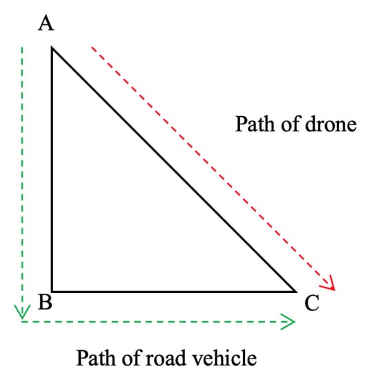
Figure 3.
Different travel distance between the drone and road vehicles with the same starting point and ending point.
5.2. First Results
We first report on the results obtained by the proposed heuristic. At this stage, we ignore the fixed costs for positioning the drone—we only consider the transportation costs (by road and by air). Later, we expand our analysis to consider this aspect. Since the stating step of our heuristic is randomized, we repeated 15 times the procedure for each instance, saving the best solution and the corresponding information.
In Table 1 and Table 2, we present the results for the 50-node and 100-node instances, respectively. In these tables, the first column specifies the instance. The following six columns indicate how the demand nodes were distributed among the road vehicles (Nv) and the drone (Nd). The column headed with Cv indicates the total transportation cost associated with the fleet of road vehicles and Cd is the total delivery cost for the drone. Ct is just the sum of the previous costs, i.e., the total delivery cost. Ct1 is the total transportation cost for the first-phase solution. Finally, the last column contains the CPU time required to obtain the reported solution.

Table 1.
Heuristic solutions for the 50-node instances.
Table 2.
Heuristic solutions for the 100-node instances.
By observing Table 1, Table 2 and Table 3, we conclude that the initial solution obtained without considering the drone is improved in the second phase, indicating a clear benefit from using this alternative transportation mode. - can be regarded as the system cost after adding the drone, and - is the cost before adding the drone. Through calculation, it can be seen that when the number of demand points is 50, 100 and 200, the cost is reduced by 12.96%, 7.16% and 8.49% due to the addition of drone, respectively. This means that the drone can bring incur cost savings of approximately 10%.
Table 3.
Heuristic solutions for the 200-node instances.
Observing the above tables, we also realize that the proposed heuristic approach quickly leads to a feasible solution within 2s (for the tested instances). This is relevant in modern logistics systems when decisions need to be made quickly upon receiving a set of customer orders.
For a small number of demand nodes, our problem can be solved up to proven optimality using a general-purpose solver. This fact allows us to assess the quality of our heuristic for at least a few small instances. We considered the MIP solver of IBM ILOG CPLEX release 12.10. Unfortunately, the instances presented in Section 5.1 are too large for the plain use of a general solver. For this reason, we used the same methodology as before to generate a few smaller instances: we generated instances with 12, 15 and 20 demand nodes. Five instances were generated in each case. In all cases, two drone stations were assumed.
In Table 4, we present the obtained results. Observing this table, we see that as the number of nodes grows, the CPU time required by the solver significantly increases. In terms of the quality of the solutions provided by the heuristic, we observe that an average percentage gap of 7.89%, 9.00% and 8.85% was obtained for 12-, 15- and 20-node instances, respectively. Although the above values are high, we note that the solution time of the heuristic algorithm does not significantly increase with the increase in the scale of customer points, and the accuracy does not decrease. This means that in reality, when there are large-scale packages to be processed, calculation does not require a significant amount of time, which increases the time for service and improves customer satisfaction.
Table 4.
Result comparison of the CPLEX and heuristic algorithm.
In Table 5, we provide some information allowing a comparison between our work and those most closely related in the literature. Because this paper is different from the research of other scholars in terms of the use mode of drone, it is difficult to compare the accuracy of each algorithm, so we can only compare the performance of the algorithm in time efficiency. We recall that the TSP-D model proposed by Yurek et al. (2018) [32] includes a road vehicle and a drone. The results presented in that work indicate that the heuristic proposed by those authors tackles instances with up to 12 customer points within a reported CPU time of . In the MTSP-D problem investigated by Kitjacharoenchai et al. (2019) [35], there are multiple road vehicles and a drone. The authors reported that the heuristic they proposed finds feasible solutions for instances with 5 vehicles, 1 UAV and 50 demand nodes within . Finally, the capacitated vehicle routing problem studied by Gambella et al. (2018) [25] involves one helicopter docked on a ship. This is a problem in which the function of the helicopter is similar to that of the drone in our work, which explains why we also quote that paper. The authors designed an exact algorithm that can solve instances with up to 11 demand nodes within .
Table 5.
Result comparison with the closest related studies in the literature.
5.3. Additional Insights
In this section, we provide some additional insights into the results. First, we investigated the impact of the number of drone stations and their cost. Afterwards, we discussed the role of the drone speed.
5.3.1. Number of Drone Stations
To investigate the impact of the number of drone stations on the results, we designed two additional trials. In the first one, we fixed the number of demand nodes (N) at 100, and considered 8 and 4 stations(S). In the second trial, we fixed the number of demand nodes at 50, and assumed 4 and 2 stations. The remaining parameters were obtained as explained in Section 5.1.
The results can be observed in Table 6. When the number of drone stations increases, the drone usage also increases. This is explained by the reduction in the travel distance between the drone and the demand nodes when more stations are available. In turn, this helps reduce the delivery cost.
Table 6.
Additional insights: the role of .
Thus far, we ignored the fixed cost of using the drone stations. The results we obtained thus far help us analyze this cost component. If the fixed cost of using a drone station is too high then the savings obtained by using the drone can easily vanish. The results in Table 6 help us to foresee what are reasonable costs for the stations that compensate their use. For instance, considering instance 8, we see that the estimated reduction obtained in the total transportation cost by using the drone vanishes for a fixed station cost slightly above 4000.
5.3.2. The Impact of the Drone Speed
One assumption we made when generating the test bed data was that the drone delivery cost is negatively related to the delivery time. For this reason, it is relevant to investigate the impact on the results of the relation between the drone speed and the van speed. For this purpose, three sets of controlled trials were designed. In the first set, the speed of the drone is set to 200% of the van’s speed (instances 1–5); in the second set trials, the unit cost of the drone is set to 150% of the van’s unit cost (instances 6–10); finally, for the third set, we assume that the speed of the drone and van are the same (instances 11–15). The number of demand nodes was fixed equal to 50 and four drone stations were considered. The results are summarized in Table 7. In this table, the column headed with Vd:Vv contains the ratio between the speed of the drone and that of the van.
Table 7.
Impact of drone versus road vehicle speed.
Observing the results, we conclude that when the speed of the drone is 200% the speed of the van, the use of the drone leads to a significant decrease in the total transportation cost—whilst the number of demand nodes visited by the drone increases significantly. In this case, we also observe that the negative correlation assumed between the delivery cost and the delivery time leads to a total cost reduction of approximately 20%.
When the speed of the drone is 150% more than that of the van, the number of demand nodes visited by the drone is approximately equal to ten, and the cost of the entire distribution system is reduced by approximately 10%.
Finally, we can hardly see a significant reduction in the total delivery time when the drone and the van have similar speeds. This is an indication that when the van is not much affected by traffic congestion, it may compensate to use it more intensely, which is of course encouraged by the economies of scale associated with road delivery.
6. Conclusions
In this paper, a multiple traveling salesman problem was combined with a location-allocation problem in the context of a multi-mode last-mile logistics distribution system. The contributions of this paper include: (1) A traditional delivery mode making use of a set of road vehicles (vans) was combined with the use of a drone. Considering some factors, instead of directly deploying the drone from the road vehicle, we used trucks to transport the drones and parcels to the preset station and then the drone was sent to the customer service point. Trucks thus move between the stations with drones. (2) An integer programming model was proposed for the problem. In the model, we fully consider the synchronization of the drone and vans’ path planning. (3) A two-phase heuristic algorithm was also developed for finding feasible solutions to the problem in a short time. In the algorithm, according to the mechanism framework of cost saving, we can achieve the ideal result by exchanging the way that demand points are served (by drone or vans).
Our results show that under some circumstances (e.g., a large number of demand nodes, a higher speed of the drone compared to the road vehicle, and the relatively small cost of using the drone stations), the total transportation cost can significantly decrease by considering drone delivery. This will save approximately 10% of the cost. Our results also show that using an approximate procedure such as the proposed heuristic may be inevitable since the use of a general purpose solver is rather limited and hardly becomes a possibility for 20 or more demand nodes.
This work opens up several research avenues. First, it would be interesting to investigate an extension of the problem considering a fleet of drones (possibly with heterogeneous capacity). In keeping with this extension, it would also be interesting to consider a TSP for every drone-carrying vehicle so that a route is designed for every drone to visit a set of drone stations. It is also worth investigating the vehicle routing extension of the investigated problem by considering non-unit demands and capacitated road vehicles. The inclusion of time as a dimension of the problem is also worth studying. In particular, this would allow considering time-windows for the deliveries as well as the recharging time of the drones at the drone stations.
Overall, our work suggests new planning opportunities stemming from the better use of certain technologies, such as drone-carrying vehicles, for improving the performance of last-mile delivery operations. Future research directions include adding more constraints to the current model to make it more suitable for application scenarios under real conditions, such as the time window when operating the drone under different conditions, the capacity of the drone and battery capacity. In terms of algorithms, heuristic algorithms are designed to be more accurate and effective to solve this problem.
Author Contributions
Conceptualization, C.W. and H.L.; Formal analysis, C.W. and H.L.; Investigation, C.W.; Methodology, C.W. and Y.C.; Software, C.W. and F.S.-d.-G.; Supervision, H.L.; Validation, C.W.; Writing—original draft, C.W.; Writing—review and editing, H.L., F.S.-d.-G. and Y.C. All authors have read and agreed to the published version of the manuscript.
Funding
This research was funded by the Key Program National Natural Science Foundation of China (grant number 71831001), National Natural Science Foundation of China (grant number 72171016) and National Funding from FCT—Fundação para a Ciência e Tecnologia, Portugal (grant number UIDB/04561/2020).
Acknowledgments
This research was supported by the Beijing Logistics Informatics Research Base.
Conflicts of Interest
The authors declare no conflict of interest.
References
- Figliozzi, M. Lifecycle modeling and assessment of unmanned aerial vehicles (drones) co2e emissions. Transp. Res. Part D Transp. Environ. 2017, 57, 251–261. [Google Scholar] [CrossRef]
- Goodchild, A.; Toy, J. Delivery by drone: An evaluation of unmanned aerial vehicle technology in reducing co2 emissions in the delivery service industry. Transp. Res. Part D Transp. Environ. 1984, 61, 58–67. [Google Scholar] [CrossRef]
- Applegate, D.; Bixby, R. The Traveling Salesman Problem: A Computational Study; Chvátal, V., Cook, W., Eds.; Princeton University Press: Princeton, NJ, USA, 2006. [Google Scholar]
- Cook, W. Pursuit of the Traveling Salesman: Mathematics at the Limits of Computation; Princeton University Press: Princeton, NJ, USA, 2012. [Google Scholar]
- Nagata, Y.; Kobayashi, S. A powerful genetic algorithm using edge assembly crossover for the traveling salesman problem. INFORMS J. Comput. 2013, 25, 346–363. [Google Scholar] [CrossRef]
- Ozden, S.; Smith, A.; Gue, K. Solving large batches of traveling salesman problems with parallel and distributed computing. Comput. Oper. Res. 2017, 85, 87–96. [Google Scholar] [CrossRef] [Green Version]
- Concorde TSP Solver. Available online: http://www.math.uwaterloo.ca/tsp/concorde/ (accessed on 7 August 2020).
- Staněk, R.; Greistorfer, P.; Ladner, K.; Pferschy, U. Geometric and lp-based heuristics for angular travelling salesman problems in the plane. Comput. Oper. Res. 2019, 108, 97–111. [Google Scholar] [CrossRef]
- Coutinho, W.; Nascimento, R.; Pessoa, A.; Subramanian, A. A branch-and-bound algorithm for the close-enough traveling salesman problem. INFORMS J. Comput. 2016, 28, 752–765. [Google Scholar] [CrossRef] [Green Version]
- Wang, X.; Golden, B.; Wasil, E. A steiner zone variable neighborhood search heuristic for the close-enough traveling salesman problem. Comput. Oper. Res. 2019, 101, 200–219. [Google Scholar] [CrossRef]
- Carlsson, J.; Behroozi, M.; Mihic, K. Wasserstein distance and the distributionally robust tsp. Oper. Res. 2018, 66, 1603–1624. [Google Scholar] [CrossRef] [Green Version]
- Givens, C.; Shortt, R. A class of wasserstein metrics for probability distributions. Mich. Math. J. 1984, 31, 231–240. [Google Scholar] [CrossRef]
- Montero, A.; Méndez-Díaz, I.; Miranda-Bront, J. An integer programming approach for the time-dependent traveling salesman problem with time windows. Comput. Oper. Res. 2017, 88, 280–289. [Google Scholar] [CrossRef]
- Malaguti, E.; Martello, S.; Santini, A. The traveling salesman problem with pickups, deliveries, and draft limits. Omega 2018, 74, 50–58. [Google Scholar] [CrossRef]
- Errico, F.; Crainic, T.; Malucelli, F.; Nonato, M. A benders decomposition approach for the symmetric tsp with generalized latency arising in the design of semiflexible transit systems. Transp. Sci. 2017, 51, 706–722. [Google Scholar] [CrossRef] [Green Version]
- Gupta, A.; Nagarajan, V.; Ravi, R. Approximation algorithms for optimal decision trees and adaptive tsp problems. Math. Oper. Res. 2017, 42, 876–896. [Google Scholar] [CrossRef] [Green Version]
- Bektaş, T. The multiple traveling salesman problem: An overview of formulations and solution procedures. Omega 2006, 34, 209–219. [Google Scholar] [CrossRef]
- Zhou, H.; Song, M.; Pedrycz, W. A comparative study of improved ga and pso in solving multiple traveling salesmen problem. Appl. Soft Comput. 2018, 64, 564–580. [Google Scholar] [CrossRef]
- Soylu, B. A general variable neighborhood search heuristic for multiple traveling salesmen problem. Comput. Ind. Eng. 2015, 90, 390–401. [Google Scholar] [CrossRef]
- Xu, Z.; Rodrigues, B. An extension of the christofides heuristic for the generalized multiple depot multiple traveling salesmen problem. Eur. J. Oper. Res. 2017, 257, 735–745. [Google Scholar] [CrossRef]
- Christofides, N. Worst-Case Analysis of a New Heuristic for the Traveling Salesman Problem; Technical Report; CS-93–13; Carnegie-Mellon University: Pittsburgh, PA, USA, 1976. [Google Scholar]
- Bektaş, T. Formulations and benders decomposition algorithms for multidepot salesmen problems with load balancing. Eur. J. Oper. Res. 2012, 216, 83–93. [Google Scholar] [CrossRef]
- Kota, L.; Jarmai, K. Mathematical modeling of multiple tour multiple traveling salesman problem using evolutionary programming. Appl. Math. Model. 2015, 39, 3410–3433. [Google Scholar] [CrossRef]
- Dhein, G.; Neto, A.; de Araújo, O. The multiple traveling salesman problem with backup coverage. Electron. Notes Discret. Math. 2018, 66, 135–142. [Google Scholar] [CrossRef]
- Gambella, C.; Lodi, A.; Vigo, D. Exact solutions for the carrier-vehicle traveling salesman problem. Transp. Sci. 2018, 52, 320–330. [Google Scholar] [CrossRef]
- Erdoğan, G.; Yldrm, E.A. Exact and heuristic algorithms for the carrier–vehicle traveling salesman problem. Transp. Sci. 2021, 55, 101–121. [Google Scholar] [CrossRef]
- Azar, A.T.; Koubaa, A.; Ali Mohamed, N.; Ibrahim, H.A.; Ibrahim, Z.F.; Kazim, M.; Ammar, A.; Benjdira, B.; Khamis, A.; Hameed, I.A.; et al. Drone Deep Reinforcement Learning: A Review. Electronics 2021, 10, 999. [Google Scholar] [CrossRef]
- Luo, C.; Du, Z.; Yu, L. Neural Network Control Design for an Unmanned Aerial Vehicle with a Suspended Payload. Electronics 2019, 8, 931. [Google Scholar] [CrossRef] [Green Version]
- Murray, C.; Chu, A. The flying sidekick traveling salesman problem: Optimization of drone-assisted parcel delivery. Transp. Res. Part C Emerg. Technol. 2015, 54, 86–109. [Google Scholar] [CrossRef]
- Carlsson, J.; Song, S. Coordinated logistics with a truck and a drone. Manag. Sci. 2018, 64, 4052–4069. [Google Scholar] [CrossRef] [Green Version]
- Agatz, N.; Bouman, P.; Schmidt, M. Optimization approaches for the traveling salesman problem with drone. Transp. Sci. 2018, 52, 965–981. [Google Scholar] [CrossRef]
- Yurek, E.; Ozmutlu, H. A decomposition-based iterative optimization algorithm for traveling salesman problem with drone. Transp. Res. Part C Emerg. Technol. 2017, 91, 735–745. [Google Scholar] [CrossRef]
- Ha, Q.; Deville, Y.; Pham, Q.; Ha, M. On the min-cost traveling salesman problem with drone. Transp. Res. Part C Emerg. Technol. 2018, 86, 597–621. [Google Scholar] [CrossRef] [Green Version]
- Pina-Pardo, J.; Silva, D.; Smith, A. The traveling salesman problem with release dates and drone resupply. Comput. Oper. Res. 2021, 129, 105–170. [Google Scholar] [CrossRef]
- Kitjacharoenchai, P.; Ventresca, M.; Moshref-Javadi, M.; Lee, S.; Tanchoco, J.; Brunese, P. Multiple traveling salesman problem with drones: Mathematical model and heuristic approach. Comput. Ind. Eng. 2019, 129, 14–30. [Google Scholar] [CrossRef]
- Ham, A. Integrated scheduling of m-truck, m-drone, and m-depot constrained by time-window, drop-pickup, and m-visit using constraint programming. Transp. Res. Part C Emerg. Technol. 2018, 91, 1–14. [Google Scholar] [CrossRef]
- Kim, S.; Lim, G.; Cho, J. Drone flight scheduling under uncertainty on battery duration and air temperature. Comput. Ind. Eng. 2018, 117, 291–302. [Google Scholar] [CrossRef]
- Hartigan, J.; Wong, M.A. Algorithm as 136: A k-means clustering algorithm. J. R. Stat. Soc. Series C Appl. Stat. 1979, 28, 100–108. [Google Scholar] [CrossRef]
- Aloise, D.; Hansen, P.; Liberti, L. An improved column generation algorithm for minimum sum-of-squares clustering. Math. Program. A 2012, 131, 195–220. [Google Scholar] [CrossRef] [Green Version]
- Gribel, D.; Vidal, T. HG-means: A scalable hybrid genetic algorithm for minimum sum-of-squares clustering. Pattern Recognit. 2019, 88, 569–583. [Google Scholar] [CrossRef] [Green Version]


Publisher’s Note: MDPI stays neutral with regard to jurisdictional claims in published maps and institutional affiliations. |
© 2021 by the authors. Licensee MDPI, Basel, Switzerland. This article is an open access article distributed under the terms and conditions of the Creative Commons Attribution (CC BY) license (https://creativecommons.org/licenses/by/4.0/).