Abstract
The main objective of this work was to find the most efficient method to interpolate metal oxide gas sensor used in a pulsed-temperature operating mode. This pulsed thermal profile is obtained by applying 6 power steps of 2 s each on the heater resistor. The experimental values of the sensing layer resistance, with a sampling time of 4ms, were interpolated by using two different static methods: a polynomial modelling and a neural network modelling, and one dynamic method: the diffusive representation. Then, the results have been compared in terms of precision and number of useful output data, as minimum as possible for high performance and rapid data treatment which is great of interest in embedded systems. The best results are obtained with the diffusive representation; it allows converting 500 measurements into 11 output coefficients.
1. Introduction
Metal-oxide thin film sensors have been widely used for gas sensing applications thanks to their sensitivity toward a large variety of gases [1]. Modulating the temperature of a micro-hotplate gas sensor allows increasing the sensitivity and/or selectivity toward various gases [2,3,4,5,6,7,8,9,10,11,12,13,14]. In some cases, the transient behavior of the sensing resistance, located just after a temperature change, is used to discriminate gases by comparing signal shapes [10,11]. In these cases, it is necessary to use powerful interpolation systems associated with mathematical analysis, as discriminant factorial analysis or neural network for example [15,16,17,18,19,20,21,22,23]. Many studies have tried to model the sensors responses by physical or physico-chemical models, but always for thermodynamically stable behaviors, that is to say at a constant temperature or variation until steady state [24,25,26]. It is almost impossible in pulsed mode, hence the interest of using mathematical modeling or interpolation.
As soon as a temperature-modulated mode and a decision-making system have been employed, a behavioral model is required to link them. Thus, the sensitive resistance response curves must be interpolated before being injected into the decision-making system. Mathematical models, as polynomial and neural network models, are commonly used to realize this stage [27,28,29,30,31,32,33,34]. In our study, a fractional model, usually employed in several domains (control systems, electromechanical systems, electronics,…), called diffusive representation [35,36] will be compared to two standard mathematical models. The greatest difficulty to interpolate the signal is due to the high nonlinearity created by the transition between the fast thermal effect at the beginning of the step (during the first 100 ms) and the slow diffusive effect (during the rest of the step). The interpolation principle of the gas sensor response is shown in Figure 1.
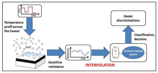
Figure 1.
Interpolation principle of the gas sensors response.
2. Experimental
2.1. Micro-Hotplate Metal Oxide Gas Sensor
A micro-heater structure has been developed and optimized at LAAS-CNRS in order to be able to work until 550 °C with low power consumption (55 mW at 550 °C) and with very low response time (or thermal inertia). The platform consists of a silicon bulk on which a thermally resistive bilayer SiO2/SiNx was grown (with low residual stress). Afterwards, a platinum metallization was realized by lift-off to define a heating resistor. Contacts were opened in a previously deposited SiO2 passivation layer. Then, platinum electrodes of the sensing resistor were deposited by evaporation. Finally, the rear side of the bulk was etched to release the membrane in order to increase the thermal resistance and then to limit thermal dissipation. It is then possible to deposit a gas sensitive layer as various metal-oxide layer to form the sensing thin film resistor. Pictures of the final component are presented in Figure 2.
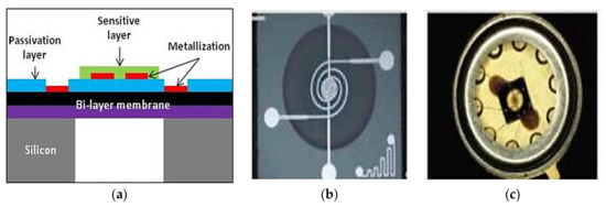
Figure 2.
Micro-hotplate gas sensor: (a) cross sectional view, (b) chip top view, (c) chip packaged on a TO-5 support.
2.2. Experimental Setup
The sensors are placed into a test chamber where gas is flowing as shown in Figure 3. The composition and relative humidity rate of the gas mixture are controlled by Mass Flow Controllers and the global flow rate is checked at the outlet with a flowmeter. The heating and the sensing resistors are connected to an acquisition boards able to control simultaneously the power applied to the heater and measure the sensitive layer resistance. The sensing resistor measurement sampling period is 4 ms. The whole test bench is automatically controllable thanks to a suitable interface and a dedicated software.
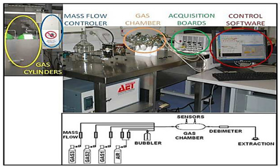
Figure 3.
Picture and diagram of the test bench.
2.3. Experimental Protocol
An optimized temperature-modulated profile applied to the heater resistance has been studied. The optimization has consisted in finding the profile that permits the fastest stabilization of the sensor and the best gas discrimination with the different steps. The profile consists in 6 steps, with a reference applied power fixed at 55 mW that corresponds to the highest temperature usable (550 °C) (calibrated by IR camera measurements). Between each reference step, a lower power step is applied. The 3 steps of power are 45 mW (400 °C), 35 mW (300 °C) and 25 mW (200 °C), for the second, fourth and sixth step respectively. As the duration of each step is 2 s, the total number of sample is 500 for each step (3000 samples per cycle). This cycle of 6 steps is continuously repeated throughout the test under various sequential atmospheres (air, CO, air, C3H8, air, NO2, air, and then combination of mixtures). The profile applied to the micro-heater and the corresponding sensitive resistance response under air (as an example) are presented in Figure 4. The different shapes of transient responses under different gases have been presented in [11].
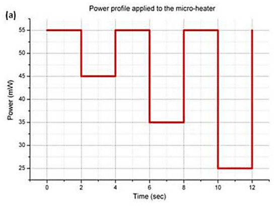
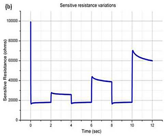
Figure 4.
Power profile applied to the heater (a) and example of sensitive resistance variations under air (b).
3. Results and Discussion
In order to simplify the output data of the sensing resistor, several models have been studied: two well known mathematical modeling (polynomial and neural network) and an approach based on a linear modeling (diffusive representation). Each model was compared with the output data and the quantity of useful coefficients introduced by each type of model was investigated (to minimize them).
3.1. Polynomial Modeling
The first mathematical interpolation considered is the polynomial modeling. It applies to many cases and its interest lies in its simplicity. This model allows interpolating very difficult curves by increasing the order of the polynomial used. With this technique, it is possible to deal with problems of very complex modeling without any prior knowledge on the dataset. It is widely used to determine empirical laws from experimental measurements.
There are several software for the calculation of numerical coefficients; in our case, we used Matlab with the “Curve Fitting Toolbox”. We worked on the data presented in the Figure 4. The interpolation is done for each step separately. The minimum polynomial order used is 9 to approximate correctly experimental data but it is also the highest degree available in this toolbox. The lower levels give worse results. The obtained results are shown in Figure 5.
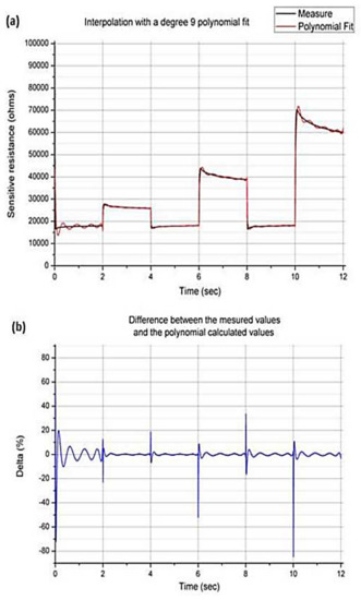
Figure 5.
Comparison between the sensor’s response and the polynomial modeling (a) and difference between both (b).
A very high drift between the sensor’s response and the polynomial modeling, located in the first one hundred milliseconds after each step transitions, is observed. The maximum drift is around 85% and the mean drift is close to 2%. This method is not suitable for this type of curve because the drift values are too high, especially in the first hundred milliseconds where the maximum information for discrimination is located.
3.2. Neural Network Modelling
Another well known interpolation technique is the use of a neural network. There are many different networks, depending on the application and in the case of interpolation, the most suitable is called “Feed Forward” network without backpropagation as presented in Figure 6.
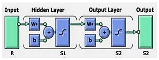
Figure 6.
Neural network commonly used for interpolation.
The results presented were obtained with the “Neural Fitting Toolbox” of Matlab. The architecture is defined according to the number of hidden neurons (S1) and the number of output neurons (S2). According to a study done on several different architectures, the best results were obtained using 50 hidden neurons and one output neuron. The interpolation obtained with 50 hidden neurons is shown in Figure 7.
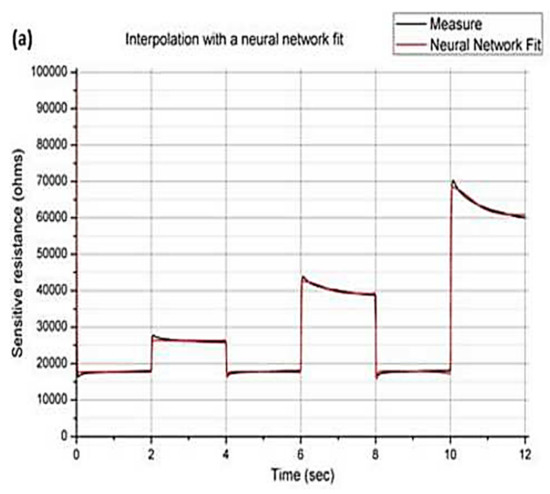
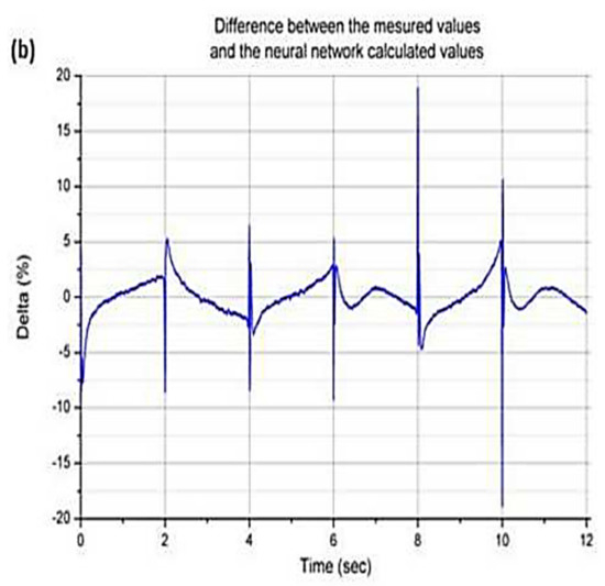
Figure 7.
Comparison between the sensor’s response and the neural network modeling (with 50 hidden neurons) (a) and difference between both (b).
The greatest difference between the sensor’s response and the modeling by neural network is, as in the case of the polynomial modeling, in the first hundred milliseconds after each step transition. However, the maximum relative difference is only around 19% and the mean value is close to 1.2%.
This model could be interesting (more suitable than the polynomial model) for interpolation of our transient curves but the number of hidden neurons is very high. A neural network with 50 hidden neurons and one output neuron represents a total of 102 different coefficients to be treated. In other words, it is necessary to use 102 coefficients to describe 500 measurement points. For the use of a decision-making system, the descriptor level measurement is divided by 5, but it’s still a lot of variables. Another point is the calculation programming of the neural network. Such an algorithm, with a hundred coefficients, can be heavy computation time. Indeed, convergence loops are used during the learning in order to adapt the input to the output according to the coefficients. The time to reach the target values can be long depending on the shape of the curves.
3.3. Diffusive Representation
3.3.1. Model Presentation
The linear modeling studied uses the concept of “diffusive representation”. A physical system that contains dynamic phenomena can be approximated by an operator as defined by following Equation (1).
where H is the operator, μ the diffusive representation function, ξ the frequency variable, and p the Laplace variable. A diffusive nature physical system can be expressed as an infinite sum of fractions as defined in the Laplace domain. It has been shown that it was possible to simplify the representation of linear dynamic inputs/outputs [37,38]. We were interested in the use of the concept of linear system inputs/outputs for the modeling and identification of these coefficients [39] for the dynamic responses of our gas sensors.
These responses can be considered as an image of a superposition of several different physical phenomenon (chemical reactions, grain boundary barriers, thermionic emission, …). The system thus has a fractional character: it is the sum of several phenomena with different time constants, low values (surface chemical reactions, thermal transition resistance heating) as high values (diffusion phenomena). It is for these reasons that the first polynomial model doesn’t work. That’s why we found interesting to use the diffusive model to represent the sensor response as a linear dynamic model of input-output.
A state-space model has been chosen to represent the system. As presented in Figure 8, the model consists in connecting the input and output with intermediate variables called state variables (physical phenomenon uncorrelated variables). The complexity of the model is then defined by the number of state variables used.
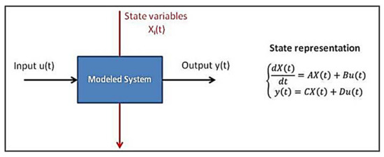
Figure 8.
State-space model.
In the previous picture, A, B, C and D are matrices of the model coefficients, and X is the vector of the state variables.
3.3.2. Used Model
The purpose of the method is equivalent to identify the following equation system 2 with a set of experimental inputs/outputs.
The simplicity of the model lies in the fact that only the function μ(ξ) is determining for system identification. But we have two problems with regard to this expression with our application. First, in our case, the t variable is not continuous (one point each 4 ms). Secondly, a real signal has an infinite spectrum (from zero to infinity), but as our measure is sampled, the recorded signal does not contain all frequencies. This implies that we have to determine a finite number of frequencies ξ and the integration limits must be finished to solve this model numerically. The initial model can be approximated by the following discrete system (3).
In this form, the system can be solved by defining the model order N, the values of ξ and using our data inputs/outputs measured. After some calculations, a simple expression for the calculation of state variables is obtained (4).
The following Equation (5) is derived from the system (3) for the direct calculation of the vector μ (specific for the identification of our model).
The vector C(n) is defined according to the state-space representation (Figure 8). The calculation of this vector is derived from Equation (4).
where M is the number of measurements equal to M = Tf − Ti/ΔT, Tf final time, Ti initial time, ΔT sampling period.
Once identified the specific distribution μ, we can calculate the output simulated by the model (7).
In summary, the use of this model can be summarized in three main steps:
- To set the system order (N). It is the number of state variables X and the number of values ξ.
- To define ξ, specific variables to the frequency domain. We have to define the number of decades on which our model is used (respecting the Shannon’s theorem). Then, we calculate the values of our vector for the number N, between frequencies terminals defined, for a logarithmic spacing between points.
- To provide a set of input/output measurements.
3.3.3. Model Optimizations
In order to optimize the modeling, two parameters have been studied for each step of the profile: the number of decades used (D) and the system order (N).
First, the number of decades used has been investigated. To conduct this study, the system order has been set to 10 and the behavior of the model for three decades amounts (1, 3 and 5) has been observed. The results are reported in Figure 9. The best result, in all cases, is obtained with 3 decades. Higher values were also tested, but the signal deteriorates rapidly.
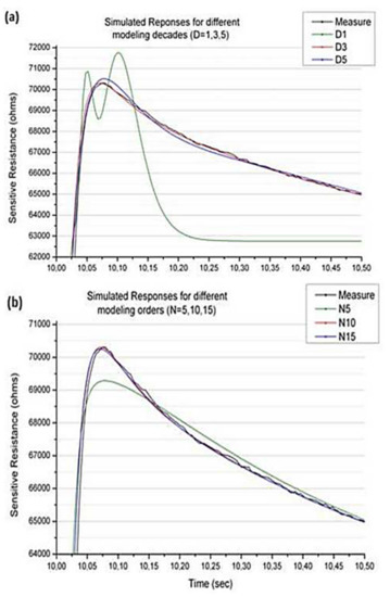
Figure 9.
Simulated responses for different modeling decades (a) and different modeling orders (b).
Then, the system order has been considered. The decades amount has been set to 3 and 3 orders (5, 10 and 15) have been studied. The results are also reported in Figure 9. The best result, for all steps, is obtained with an order system equal to 10.
Since the order system was set at 10, this new model only consists of 11 coefficients: 10 values of μ and Y0.
3.3.4. Model Performance for the Interpolation
Now that we have optimized the performance of this model (3 decades and the order of the system equal to 10), we can implement it in Matlab and compare these results to those of the actual output. Overlayed curves and the difference between both are given in the following graphs (Figure 10).
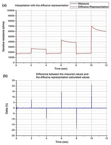
Figure 10.
Comparison between the sensor’s response and the diffusive representation modeling (a) and difference between both (b).
The greatest difference between the sensor’s response and the diffusive representation is located, as in the case of previous modeling, in the first hundred milliseconds after each step transitions. The maximum deviation is around 21% and the mean value is close to 0.1%. So, in addition to allowing a large variables reduction (11 coefficients in place of 500 measurement points), this model is very faithful to the actual response of the sensor. Results are better than the neural network and the number of values is reduced by 50 (instead of 5 with the neural network). Moreover, the calculations to be carried out with this model are matrix calculations, whereas they are convergence loops in the case of the neural network; therefore the calculations are much faster with the diffusive representation.
4. Conclusions
The ability to significantly reduce the amount of sensing resistor output variables of a metal-oxide gas sensor has been investigated. Three different methods were tested: two static methods with the polynomial modeling and the neural network modeling, and one dynamic method with the diffusive representation. The first model has proven not to be adapted to our data (high values of maximum and average deviation). The second was more effective but the amount of coefficient was too high (102 coefficients instead of 500 measurement points). Finally, the diffusion representation proved to be the best candidate for the data modeling: A very faithful interpolation with only 11 coefficients based on a fast matrix calculation. Moreover, this modelling is easily implementable with many other kind of sensors (not only for gas sensors) in a real time systems, and it presents the advantage of being a dynamic (with another input, the modeling is still good) and linear (the output is linear towards the input) system.
Future work will therefore focus on the use of these data with a decision-making system under different gases.
Author Contributions
Conceptualization, G.G. and G.M.; Data curation, C.T. (Cyril Tropis) and N.D.; Resources, C.T. (Chaabane Talhi) and F.B.; Software, B.F.; Writing—review & editing, G.G. and P.M. All authors have read and agreed to the published version of the manuscript.
Funding
This research received no external funding.
Institutional Review Board Statement
Not applicable.
Informed Consent Statement
Informed consent was obtained from all subjects involved in the study.
Data Availability Statement
The data can be available on HAL-LAAS thanks to “MDPI Research Data Policies” at https://www.mdpi.com/ethics (accessed on 15 October 2021).
Acknowledgments
This work was supported by LAAS-CNRS micro and nanotechnologies platform, a member of the Renatech french national network.
Conflicts of Interest
The authors declare no conflict of interest.
References
- Wang, C.; Yin, L.; Zhang, L.; Xiang, D.; Gao, R. Metal oxide gas sensors: Sensitivity and influencing factors. Sensors 2010, 10, 2088–2106. [Google Scholar] [CrossRef]
- Burresi, A.; Fort, A.; Rocchi, S.; Serrano, B.; Ulivieri, N.; Dynamic, V.V. CO recognition in presence of interfering gases by using one MOX sensor and a selected temperature profile. Sens. Actuators B 2005, 106, 40–43. [Google Scholar] [CrossRef]
- Cavicchi, R.E.; Suehle, J.S.; Kreider, K.G.; Gaitan, M.; Chaparala, P. Optimized temperaturepulse sequences for the enhancement of chemically specific response patterns from microhotplate gas sensors. Sens. Actuators B 1996, 33, 142–146. [Google Scholar] [CrossRef]
- Schweizer-Berberich, M.; Zdralek, M.; Weimar, U.; Göpel, W.; Viard, T.; Martinez, D.; Seube, A.; Peyre-Lavigne, A. Pulsed mode of operation and artificial neural network evaluation for improving the CO selectivity of SnO2 gas sensors. Sens. Actuators B 2000, 65, 91–93. [Google Scholar] [CrossRef]
- Montoliu, I.; Tauler, R.; Padilla, M.; Pardo, A.; Marco, S. Multivariate curve resolution applied to temperature-modulated metal oxide gas sensors. Sens. Actuators B 2010, 145, 464–473. [Google Scholar] [CrossRef]
- Lee, A.P.; Reedy, B.J. Temperature modulation in semiconductor gas sensing. Sens. Actuators B 1999, 60, 35–42. [Google Scholar] [CrossRef]
- Hosseini-Golgoo, S.M.; Hossein-Babaei, F. Assessing the diagnostic information in the response patterns of a temperature-modulated tin oxide gas sensor. Meas. Sci. Technol. 2011, 22, 035201. [Google Scholar] [CrossRef]
- Hossein-Babaei, F.; Amini, A. A breakthrough in gas diagnosis with a temperature-modulated generic metal oxide gas sensor. Sens. Actuators B 2012, 166-167, 419–425. [Google Scholar] [CrossRef]
- Ponzoni, A.; Depari, A.; Comini, E.; Faglia, G.; Flammini, A.; Sberveglieri, G. Response dynamics of metal oxide gas sensors working with temperature profile protocols. Procedia Eng. 2011, 25, 1173–1176. [Google Scholar] [CrossRef]
- Varpula, A.; Novikov, S.; Haarahiltunen, A.; Kuivalainen, P. Transient characterization techniques for resistive metal-oxide gas sensors. Sens. Actuators B 2011, 159, 12–26. [Google Scholar] [CrossRef]
- Parret, F.; Menini, P.; Martinez, A.; Soulantica, K.; Maisonnat, A.; Chaudret, B. Improvement of micromachined SnO2 gas sensors selectivity by optimised dynamic temperature operating mode. Sens. Actuators B 2006, 118, 276–282. [Google Scholar] [CrossRef]
- Vergara, A.; Llobet, E.; Brezmes, J.; Ivanov, P.; Cane, C.; Gracia, I.; Vilanova, X.; Correig, X. Quantitative gas mixture analysis using temperature-modulated micro-hotplate gas sensors: Selection and validation of the optimal modulating frequencies. Sens. Actuators B 2007, 123, 1002–1016. [Google Scholar] [CrossRef]
- Ionescu, R.; Hoel, A.; Granqvist, C.G.; Llobet, E.; Heszler, P. Ethanol and H2S gas detection in air and in reducing and oxidizing ambience: Application of pattern recognition to analyse the output from temperature-modulated nanoparticulate WO3 gas sensors. Sens. Actuators B 2005, 104, 124–131. [Google Scholar] [CrossRef]
- Jaegle, M.; Wollenstein, J.; Meisinger, T.; Bottner, H.; Muller, G.; Becker, T.; Braunmuhl, C.B. Micromachined thin film SnO2 gas sensors in temperature-pulsed operation mode. Sens. Actuators B 1999, 57, 130–134. [Google Scholar] [CrossRef]
- Frietsch, M.; Zudock, F.; Goschnick, J.; Bruns, M. CuO catalytic membrane as selectivity trimmer for metal oxide gas sensors. Sens. Actuators B 2000, 65, 379–381. [Google Scholar] [CrossRef]
- Musatov, V.Y.; Sysoev, V.V.; Sommer, M.; Kiselev, I. Close-to-practice assessment of meat freshness with metal oxide sensor microarray electronic nose. AIP Conf. Proc. 2009, 1137, 469–472. [Google Scholar]
- Tomchenko, A.A.; Harmer, G.P.; Marquis, B.T.; Allen, J.W. Semiconducting metal oxide sensor array for the selective detection of combustion gases. Sens. Actuators B 2003, 93, 126–134. [Google Scholar] [CrossRef]
- Zhang, Q.; Xie, C.; Zhang, S.; Wang, A.; Zhu, B.; Wang, L.; Yang, Z. Identification and pattern recognition analysis of Chinese liquors by doped nano ZnO gas sensor array. Sens. Actuators B 2005, 110, 370–376. [Google Scholar] [CrossRef]
- Huang, J.; Wan, Q. Gas Sensors Based on Semiconducting Metal Oxide One-Dimensional Nanostructures. Sensors 2009, 9, 9903–9924. [Google Scholar] [CrossRef]
- Siripatrawan, U. Rapid differentiation between E. coli and Salmonella Typhimurium using metal oxide sensors integrated with pattern recognition. Sens. Actuators B 2008, 133, 414–419. [Google Scholar] [CrossRef]
- Setkus, A.; Olekas, A.; Senuliene, D.; Falasconi, M.; Pardo, M.; Sberveglieri, G. Featuring of odor by metal oxide sensor response to varying gas mixture. AIP Conf. Proc. 2009, 1137, 202–205. [Google Scholar]
- Yin, Y.; Tian, X. Classification of Chinese drinks by a gas sensors array and combination of the PCA with Wilks distribution. Sens. Actuators B 2007, 124, 393–397. [Google Scholar] [CrossRef]
- Lee, D.; Huh, J.; Lee, D. Classifying combustible gases using micro-gas sensor array. Sens. Actuators B 2003, 93, 1–6. [Google Scholar] [CrossRef]
- Barsan, N.; Weimar, U. Conduction Model of Metal Oxide Gas Sensors. J. Electroceram. 2001, 7, 143–167. [Google Scholar] [CrossRef]
- Barsan, N.; Weimar, U. Understanding the fundamental principles of metal oxide based gas sensors; the example of CO sensing with SnO2 sensors in the presence of humidity. J. Phys. Condens. Matter 2003, 15, 813–839. [Google Scholar] [CrossRef]
- Ding, J.; McAvoy, T.J.; Cavicchi, R.E.; Semancik, S. Surface state trapping models for SnO2-based microhotplate sensors. Sens. Actuators B 2001, 77, 597–613. [Google Scholar] [CrossRef]
- el Barbria, N.; Amaria, A.; Vinaixab, M.; Bouchikhia, B.; Correigb, X.; Llobet, E. Building of a metal oxide gas sensor-based electronic nose to assess the freshness of sardines under cold storage. Sens. Actuators B 2007, 128, 235–244. [Google Scholar] [CrossRef]
- Galdikas, A.; Mironas, A.; Senulien, D.; Strazdien, V.; Setkus, A.; Zelenin, D. Response time based output of metal oxide gas sensors applied to evaluation of meat freshness with neural signal analysis. Sens. Actuators B 2000, 69, 258–265. [Google Scholar] [CrossRef]
- Lv, P.; Tang, Z.; Wei, G.; Yu, J.; Huang, Z. Recognizing indoor formaldehyde in binary gas mixtures with a micro gas sensor array and a neural network. Meas. Sci. Technol. 2007, 18, 2997. [Google Scholar] [CrossRef]
- Vlachos, D.S.; Fragoulis, D.K.; Avaritsiotis, J.N. An adaptive neural network topology for degradation compensation of thin film tin oxide gas sensors. Sens. Actuators B 1997, 45, 223–228. [Google Scholar] [CrossRef]
- Lee, D.S.; Jung, H.Y.; Lim, J.W.; Lee, M.; Ban, S.W.; Huh, J.S.; Lee, D.D. Explosive gas recognition system using thick film sensor array and neural network. Sens. Actuators B 2000, 71, 90–98. [Google Scholar] [CrossRef]
- Fine, G.F.; Cavanagh, L.M.; Afonja, A.; Binions, R. Metal oxide semi-conductor gas sensors in environmental monitoring. Sensors 2010, 10, 5469–5502. [Google Scholar] [CrossRef]
- Balasubramanian, S.; Panigrahi, S.; Logue, C.M.; Gu, H.; Marchello, M. Neural networksintegrated metal oxide-based artificial olfactory system for meat spoilage Identification. J. Food Eng. 2009, 91, 91–98. [Google Scholar] [CrossRef]
- Srivastava, A.K. Detection of volatile organic compounds (VOCs) using SnO2 gas-sensor array and artificial neural network. Sens. Actuators B 2003, 96, 24–37. [Google Scholar] [CrossRef]
- Casenave, C. Time-local formulation and identification of implicit Volterra models by use of diffusive representation. Automatica 2011, 10, 2273–2278. [Google Scholar] [CrossRef][Green Version]
- Allard, B.; Jorda, X.; Bidan, P.; Rumeau, A.; Morel, H.; Perpina, X.; Vellvehi, M.; M’Rad, S. Reduced-order thermal behavioral model based on diffusive representation. IEEE Trans. Power Electron. 2009, 24, 2833–2846. [Google Scholar] [CrossRef]
- Montseny, G. Diffusive representation of pseudo-differential time-operators. ESAIM Proc. Fract. Differ. Syst. Models Methods Appl. 1998, 5, 159–175. [Google Scholar] [CrossRef]
- Montseny, G.; Mbodje, B. Optimal models of fractional integrators and application to systems with fading memory. Syst. Man Cybern. 1993, 5, 65–70. [Google Scholar]
- Garcia, G.; Bernussou, J. Identification of the dynamics of the lead acid battery by a diffusive model. ESAIM Proc. Fract. Differ. Syst. Models Methods Appl. 1998, 5, 87–98. [Google Scholar] [CrossRef]


Publisher’s Note: MDPI stays neutral with regard to jurisdictional claims in published maps and institutional affiliations. |
© 2021 by the authors. Licensee MDPI, Basel, Switzerland. This article is an open access article distributed under the terms and conditions of the Creative Commons Attribution (CC BY) license (https://creativecommons.org/licenses/by/4.0/).