Adaptive Robust Control for Networked Strict-Feedback Nonlinear Systems with State and Input Quantization

Abstract

Backstepping method is a successful approach to deal with the systems in strict-feedback form. However, for networked control systems, the discontinuous virtual law caused by state quantization introduces huge challenges for its applicability. In this article, a quantized adaptive robust control approach in backsetpping framework is developed in this article for networked strict-feedback nonlinear systems with both state and input quantization. In order to prove the efficiency of the designed control scheme, a novel form of Lyapunov candidate function was constructed in the process of analyzing the stability, which is applicable for the systems with nondifferentiable virtual control law. In particular, the state and input quantizers can be in any form as long as they meet the sector-bound condition. The theoretic result shows that the tracking error is determined by the pregiven constants and quantization errors, which are also verified by the simulation results.

1. Introduction

Nonlinear systems in parametric strict-feedback form with uncertainties have been investigated a lot due to their widespread applications in modeling real systems, such as chaotic systems, robot/manipulator systems, vehicle systems and so on [1,2,3,4]. The backstepping method, proposed by Petar V. Kokotovic in [5] in 1992, is a successful way to deal with the systems in strict-feedback form. Under this method, the plant can be divided into a variety of subsystems by introducing virtual control inputs, and then, a step-by-step controller is designed for the plant. As for system uncertainties that are inevitable in real systems, there are two sorts of classical schemes to design the controller, i.e., adaptive control (AC, [6]) and deterministic robust control (DRC, see [7]). These two control laws have their own advantages and disadvantages: under the AC method, the closed-loop system is asymptotically stable in the existence of uncertain parameters only, but it may lead to instability when there is disturbance; under the DRC method, uniform ultimate boundedness (UUB) is guaranteed in the case of both uncertain parameters and disturbance. In [8], adaptive robust control (ARC) was proposed by Bin Yao and Masayoshi Tomizuka, which combined the advantages of both AC and DRC. That is, not only is the UUB property guaranteed when the system is under uncertain parameters and disturbance, but also the asymptotic stability is guaranteed under the uncertain parameters only. Just about these good properties of ARC, it has been widely applied in many engineering systems [9,10,11].

In modern society, networked control systems have been widespread investigated due to their own benefits such as low installation and maintenance cost, strong anti-interference capability of the signal, easily encrypting, storing or processing and so on. These benefits give a great impetus to develop and expand its application fields, especially in power systems, vehicle industry, teleoperation and network-based process control engineering [12,13]. However, the traditional backstepping method is hard to apply to systems in strict-feedback form for the reason that in such a system, the signal transmission between controller and plant is achieved via a digital communication network (see Figure 1), which may draw into various problems, such as time delays (deterministic delays and stochastic delays, [14]), sampling [15], packet losses (off-line algorithm [16] and on-line algorithm [17]) or packet disorder [18] and signal quantization [19]. For parametric strict-feedback nonlinear systems, some of these issues have been solved well in the past few years. In [20], the time-delay problem was considered and dealt with via adaptive NN backstepping control; while in [21], the Lemma 1 solved the sampling problem, and an adaptive sampled-data control scheme was designed for a certain class of nonlinear systems. The packet losses and time delay were considered by Wang et al. in [16].

Although there have been many results for networked control systems in strict-feedback form, few results aim at signal quantization, especially state quantization [22,23,24]. In the past decades, input quantization has been widely concerned. In [25], ${\mathcal{L}}_1$ adaptive controller was put forward for a class of uncertain nonlinear system. Jing Zhou et al. designed an adaptive backstepping controller for a class of strict feedback system with quantized input signals in [26]. After that, Lantao Xing et al. further investigated the output feedback problem of systems in strict feedback form and proposed an adaptive output-feedback control scheme in [27]. Moreover, in [28], a control method based on set-valued map was presented for nonlinear systems in strict-feedback form with quantized states. However, the complexity of this method restricts its application. In addition, it may be inapplicable when there are external disturbances. In a word, it is quite necessary to propose a universal method to deal with state and input quantization problems of strict-feedback systems.

This paper focuses on a class of uncertain nonlinear systems in strict feedback form with quantized states and input feedback. An ARC law is designed for concerned systems to ensure stability and tracking performance. The main contributions are summarized as follows: Firstly, we construct a novel differentiable and positive definite Lyapunov candidate function $V(t)$ via the states of the plant and the nondifferentiable virtual control law. Then, based on the backstepping method and the proposed Lyapunov candidate function, the detailed design processes of the ARC law are given in a step-by-step way. The analysis illustrates that under the designed controller, the closed-loop system is UUB in spite of the high uncertainties and quantized errors. To verify the universality of our results, in the simulation part, we employ both uniform quantizers and logarithmic quantizers for signal quantization. Moreover, both the stability and tracking problems are considered in simulation.

This paper is organized as follows: In Section 2, the sector boundary condition is introduced and the problem formulation is illustrated. The ARC scheme based on backstepping method is designed in Section 3 for the uncertain nonlinear systems in parameter strict-feedback form with state and input quantization. The simulation part follows in Section 4, which verifies the theoretical result above. Finally, the conclusion is given in Section 5.

Notation 1.

$\mathcal{R}$ represents the field of real numbers. $\dot{•},\ddot{•},\cdots ,{•}^{(n)}$ denote for the first-order, second-order, ⋯, and nth-order derivative of $•$ with respect to time t. ${\overline{•}}_i=[•{}_1,•{}_2,\cdots ,•{}_i]$. $\parallel •\parallel$ represents the Frobenius norm of a matrix B or Euclidean norm of a vector ξ, i.e., $∥B∥=\sqrt{{\sum }_{i,j}{b}_{ij}^2}$ and $∥\xi ∥=\sqrt{{\sum }_i{\xi }_i^2}$. $B^{\top }$ denotes the transposition of B.

2. Problem Statement

Without loss of generality, consider the following SISO nonlinear system with uncertain parameters and disturbances:

$$\left\{\begin{array}{c}{\dot{x}}_i={\phi }_i^{\top }({\overline{x}}_i,t)\theta +x_{i+1}+D_i,i=1,2,\cdots ,n-1,\hfill \\ {\dot{x}}_n={\phi }_n^{\top }({\overline{x}}_n,t)\theta +u_q+D_n,\hfill \\ y=x_1,\hfill \end{array}\right.$$

(1)

where $x_1,x_2,\cdots ,x_n\in \mathcal{R}$ are the states of the system; ${\overline{x}}_i=[x_1,x_2,\cdots ,x_i];$ $\theta =[{\theta }_1,{\theta }_2,\cdots ,$${\theta }_p{]}^{\top }$, ${\theta }_i\in \mathcal{R}$ are the unknown parameters; for $i=1,2,\cdots ,n$, ${\phi }_i={\phi }_i({\overline{x}}_i,t):{\mathcal{R}}^i\times R\to {\mathcal{R}}^p$ are all known function vectors; $D_i\in \mathcal{R}$ are the unknown functions representing the time-varying disturbances and the unmodeled dynamics; $y\in \mathcal{R}$ and $u_q=Q_u(u)\in \mathcal{R}$ are the output and quantized input, respectively; $u=u(t,{\overline{x}}_{qi})\in \mathcal{R}$ is the quantized states feedback controller and $x_{qi}=Q_i(x_i)$ are the quantized states. Actually, the result in this paper can be easily generalized to the case that $x_i$ are all m-dimensional vectors.

For the requirement of later analysis, the following conditions are assumed on the plant:

Assumption 1.

The uncertain parameters ${\theta }_i$ and unknown functions $D_i,i=1,2,\cdots ,n$ are all bounded, i.e.,

$$\begin{array}{c}{\theta }_i\in [{\theta }_{imin},{\theta }_{imax}]\doteq {\Omega }_i,\left|D_i\right|\le d_i,\end{array}$$

(2)

where ${\theta }_{imin}$ and ${\theta }_{imax}$ are the lower and upper bound of ${\theta }_i$; $d_i$ are the boundary of the unknown function $D_i$. Denote ${\Omega }_{\theta }\doteq \{\theta :{\theta }_i\in {\Omega }_i\}$; ${\theta }_{max}={[{\theta }_{1max},\cdots ,{\theta }_{pmax}]}^{\top }$; ${\theta }_{min}={[{\theta }_{1min},\cdots ,{\theta }_{pmin}]}^{\top }$; and ${\theta }_m=\underset{i}{max}(|{\theta }_{imax}|,|{\theta }_{imin}|)$.

Assumption 2.

For all $i=1,2,\cdots ,n$ and ${\overline{x}}_i$, ${\phi }_i({\overline{x}}_i,t)$ is continuous differentiable up to order $n-i$ with respect to $x_j,j=1,2,\cdots ,i$ and t. Moreover, $\frac{{\partial }^{n-i}{\phi }_i}{\partial x_j^{n-i}}$ satisfy the Lipschitz condition with respect to ${\overline{x}}_i$.

Assumption 3.

The reference command $r\in \mathcal{R}$ is sufficiently smooth.

Assumption 4.

The sector boundary condition holds for both state and input quantization, i.e., for $i=1,2,\cdots ,n$ and $j=1,2,\cdots ,m$, there exist constant $0\le {\delta }_u<1$, $0\le {\delta }_{x_i}<1$, ${\varpi }_u\ge 0$ and ${\varpi }_{x_i}\ge 0$ such that

$$\begin{array}{cc}\hfill & \left|{\Delta }_u\right|=\left|u-Q_u(u)\right|\le {\delta }_u\left|u\right|+(1-{\delta }_u){\varpi }_u,\hfill \\ \hfill & \left|{\Delta }_{x_i}\right|=\left|x_i-Q_{x_i}(x_i)\right|\le {\delta }_{x_i}\left|x_i\right|+(1-{\delta }_{x_i}){\varpi }_{x_i}.\hfill \end{array}$$

(3)

Denote ${\overline{\Delta }}_{x_n}={[{\Delta }_{x_1},\cdots ,{\Delta }_{x_n}]}^{\top }$ and from (3), we have

$$\parallel {\overline{\Delta }}_{x_n}\parallel \le {\delta }_{max}\parallel x_n\parallel +{\varpi }_{max},$$

(4)

where ${\delta }_{max}=\underset{i}{max}\left\{{\delta }_{x_i}\right\}$ and ${\varpi }_{max}=\underset{i}{max}\left\{(1-{\delta }_{x_i}){\varpi }_{x_i}\right\}$

Remark 1.

It should be noted that most common quantizers meet the sector bound property (3), such as uniform quantizer (in [29]), logarithmic quantizer (in [25]), hysteresis quantizer (in [26]) and compound quantizer (in [27]). The uniform quantizer and logarithmic quantizer are listed below as two typical examples.

A. Uniform quantizer:

There are various kinds of uniform quantizers in previous papers. We introduce the midriser uniform quantizer as an example in this paper (see also in [29]).

$$Q(\xi )=\varpi \left(⌊\frac{\xi }{\varpi }⌋+\frac{1}{2}\right)$$

(5)

where the notation $\lfloor •\rfloor$ depicts the floor function and $\varpi >0$ is a known constant that determines the quantization dense. The figure of the uniform quantizer (5) is shown in Figure 2. The quantization error of (5) satisfies

$$|Q(\xi )-\xi |\le \frac{\varpi }{2},$$

(6)

which means that the sector boundary condition (3) is true with $\delta =0$.

B. Logarithmic quantizer:

As another example, the logarithmic quantizer modeled as below is considered, whose diagram is shown in Figure 3 [25].

$$Q(\xi )=\left\{\begin{array}{cc}\hfill {\xi }_i& \frac{{\xi }_i}{1+\delta }<\xi \le \frac{{\xi }_i}{1-\delta }\hfill \\ \hfill 0& 0\le \xi \le \frac{\varpi }{1+\delta }\hfill \\ \hfill -Q(-\xi )& \xi <0.\hfill \end{array}\right.$$

(7)

where ${\xi }_i={\rho }^{i-1}\varpi ,i=1,2\cdots$, $\varpi >0$ and $\rho =\frac{1+\delta }{1-\delta }$. The quantization error is

$$\begin{array}{cc}\hfill |Q(\xi )-\xi |& \le min\left(\frac{\varpi }{1+\delta },\frac{{\xi }_i}{1-\delta }-{\xi }_i\right)\le \delta \rho \left|\xi \right|+\frac{\varpi }{1+\delta }.\hfill \end{array}$$

(8)

That is, the inequality (3) is true.

Under Assumptions 1–4, the control objective is to design an adaptive robust controller for the uncertain nonlinear system (1) such that all the signals of closed-loop system are bounded and the output $y(t)$ tracks the reference command $r(t)$ with the states and inputs quantized by quantizers.

3. Main Results

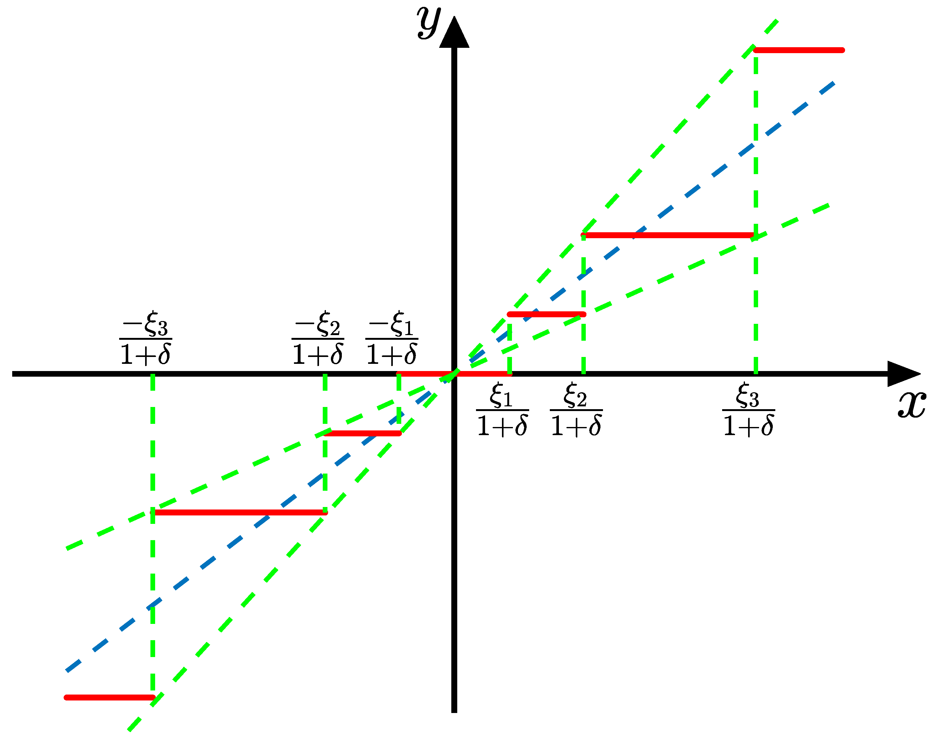
3.1. Backstepping Based Arc with Quantized States

In this section, treating the quantized errors of state signal as unmodeled dynamics, we propose an adaptive robust controller based on backstepping method for the plant (1) with state quantization only. First of all, the following lemma is necessary for the subsequent analysis.

Lemma 1.

For $i=1,2,\cdots ,n$ and any bounded set $\Omega \subset {\mathcal{R}}^i$, ${\phi }_i^{(j_1,\cdots ,j_i)}({\overline{x}}_i,t)=\frac{{\partial }^j{\phi }_i}{\partial x_1^{j_1}\cdots \partial x_i^{j_i}}$ satisfies Lipschitz condition in $\Omega$ with respect to ${\overline{x}}_i$ where $j_1,\cdots ,j_i\in {\mathcal{N}}^{+}$ and $j_1+\cdots +j_i\le n-i$, i.e., there exists a constant ${\mathcal{L}}_{j_1,\cdots ,j_i\Omega }>0$ such that for all ${\xi }_1,{\xi }_2\in \Omega$,

$$\left|{\phi }_i^{(j_1,\cdots ,j_i)}({\xi }_1,t)-{\phi }_i^{(j_1,\cdots ,j_i)}({\xi }_2,t)\right|\le {\mathcal{L}}_{j_1,\cdots ,j_i\Omega }∥{\xi }_1-{\xi }_2∥.$$

(9)

Proof. 

From Assumption 2, the lemma is true when $j_1+\cdots +j_i=n-i$. For any $j=1,2,\cdots ,i$ and $j_1+\cdots +j_i<n-i$, ${\phi }_i^{(j_1,\cdots ,j_i)}$ is continuous differentiable with respect to $x_j$. Therefore, $\frac{\partial {\phi }_i^{(j_1,\cdots ,j_i)}}{\partial x_j}$ is continuous and bounded in the set $\Omega$. That is to say, ${\phi }_i^{(j_1,\cdots ,j_i)}$ satisfies Lipschitz condition in $\Omega$ with respect to $x_j$. This leads to (9). □

Following notations are necessary for the convenience of writing.

$$\begin{array}{c}{\varphi }_i={\phi }_i-{\displaystyle \sum _{j=1}^{i-1}}\frac{\partial {\alpha }_{i-1}}{\partial x_{qj}}{\phi }_j,{\varphi }_{qi}={\varphi }_i({\overline{x}}_{qi},t),{\tilde{\varphi }}_i={\varphi }_i-{\varphi }_{qi},{\tilde{D}}_i=D_i-{\displaystyle \sum _{j=1}^{i-1}}\frac{\partial {\alpha }_{i-1}}{\partial x_{qj}}{D}_j,\\ {\beta }_i={\int }_0^t\left[\frac{\partial {\alpha }_i}{\partial t}+{\displaystyle \sum _{j=1}^i}\frac{\partial {\alpha }_i}{\partial x_{qj}}(x_{qj+1}+{\phi }_{qj}\theta +D_j)+\frac{\partial {\alpha }_i}{\partial \widehat{\theta }}\dot{\widehat{\theta }}\right]\mathrm{d}t,\\ {\tau }_i={\displaystyle \sum _{j=1}^i}{\varphi }_j{z}_j,{\tau }_{qi}={\displaystyle \sum _{j=1}^i}{\varphi }_{qj}{z}_{qj},z_i=x_i-{\beta }_{i-1},z_{qi}=x_{qi}-{\alpha }_{i-1},\end{array}$$

where ${\alpha }_0=r(t)$ and ${\alpha }_i,i\ge 1$ is the virtual control law which are designed later; $\widehat{\theta }$ is the estimation value of $\theta$. Subsequently, the design procedures are given below.

Step 1: Consider the first equation of (1). The derivative of $z_1$ is given by

$${\dot{z}}_1={\phi }_1^{\top }\theta +x_2+D_1-\dot{r}.$$

(10)

Regard $x_2$ as a virtual input, and design for it a virtual control law ${\alpha }_1(x_{q1},{\widehat{\theta }}_{\pi },t)$,

$${\alpha }_1(x_{q1},{\widehat{\theta }}_{\pi },t)=-k_1{z}_{q1}-{\varphi }_{q1}^{\top }{\widehat{\theta }}_{\pi }+\dot{r}-\frac{1}{4{\epsilon }_1}{h}_1^2{z}_{q1}$$

(11)

where $k_1>0$; ${\epsilon }_1>0$; ${\widehat{\theta }}_{\pi }=\pi (\widehat{\theta })={[{\pi }_1({\widehat{\theta }}_1),\cdots ,{\pi }_p({\widehat{\theta }}_p)]}^{\top }$ is the smooth projection mapping vector with bounded derivatives up to order $n-1$ such that

$$\left\{\begin{array}{c}\pi (\widehat{\theta })=\widehat{\theta },\forall \widehat{\theta }\in {\Omega }_{{\theta }_i},\hfill \\ \pi (\widehat{\theta })\in {\Omega }_{\widehat{\theta }},\forall \widehat{\theta }\in R^p;\hfill \end{array}\right.$$

(12)

where ${\Omega }_{\widehat{\theta }}=\left\{\nu \in R^p:{\theta }_{imin}-{\epsilon }_{{\theta }_i}\le {\nu }_i\le {\theta }_{imax}+{\epsilon }_{{\theta }_i}\right\}$, and ${\epsilon }_{{\theta }_i}>0$ is a small constant. Refer to [8], $h_1=h_1(z_{q1},{\widehat{\theta }}_{\pi },t)$ can be chosen as an any sufficiently smooth function such that

$$\begin{array}{cc}\hfill h_1\ge & \parallel {\varphi }_{q1}\parallel \parallel ({\theta }_{max}-{\theta }_{min}+2{\epsilon }_{\theta })\parallel +|D_1|+(k_1+{\mathcal{L}}_{{\varphi }_1}{\theta }_m)\left|{\Delta }_{x_1}\right|\hfill \\ \hfill \ge & |{\varphi }_{q1}^{\top }{\tilde{\theta }}_{\pi }|+|D_1|+|k_1{\Delta }_{x_1}|+|{\tilde{\varphi }}_1^{\top }\theta |,\hfill \end{array}$$

(13)

where ${\epsilon }_{\theta }={[{\epsilon }_{{\theta }_1},\cdots ,{\epsilon }_{{\theta }_p}]}^{\top }$; ${\tilde{\theta }}_{\pi }={\widehat{\theta }}_{\pi }-\theta$; ${\mathcal{L}}_{{\varphi }_1}$ is the Lipschitz constant of ${\varphi }_1$.

From Lemma 1 and Assumptions 1–3, the following lemma can be obtained spontaneously.

Lemma 2.

${\alpha }_1$, $\frac{\partial {\alpha }_1}{\partial x_1}$, $\frac{\partial {\alpha }_1}{\partial t}$ and $\frac{\partial {\alpha }_1}{\partial \widehat{\theta }}$ satisfy the Lipschitz condition with respect to $x_1$.

Consider the positive definite continuous function $V_1=\frac{1}{2}{z}_1^2$. From (10) to (13), the derivative of $V_1$ is

$$\begin{array}{cc}\hfill {\dot{V}}_1=& z_1(k_1{\Delta }_{x_1}+D_1-{\varphi }_{q1}^{\top }{\tilde{\theta }}_{\pi }+{\tilde{\varphi }}_1^{\top }\theta -\frac{1}{4{\epsilon }_1}{h}_1^2{z}_1)\hfill \\ \hfill & +z_1{z}_2-k_1{z}_1^2+z_1({\beta }_1-{\alpha }_1)+\frac{1}{4{\epsilon }_1}{h}_1^2{z}_1{\Delta }_{x_1}\hfill \\ \hfill \le & z_1{z}_2-k_1{z}_1^2+z_1({\beta }_1-{\alpha }_1+\frac{1}{4{\epsilon }_1}{h}_1^2{\Delta }_{x_1})+{\epsilon }_1.\hfill \end{array}$$

(14)

Step 2: Consider the second equation of (1). The derivative of $z_2$ is given by

$${\dot{z}}_2={\varphi }_2^{\top }\theta +x_3+{\tilde{D}}_2-\frac{\partial {\alpha }_1}{\partial t}-\frac{\partial {\alpha }_1}{\partial \widehat{\theta }}\dot{\widehat{\theta }}-\frac{\partial {\alpha }_1}{\partial x_{q1}}{x}_{q2}.$$

(15)

Regard $x_3$ as a virtual input, and design for it a virtual control law ${\alpha }_2({\overline{x}}_{q2},{\widehat{\theta }}_{\pi },t)$,

$$\begin{array}{cc}\hfill {\alpha }_2=& -k_2{z}_{q2}-z_{q1}-{\varphi }_{q2}^{\top }{\widehat{\theta }}_{\pi }+\frac{\partial {\alpha }_1}{\partial t}+\frac{\partial {\alpha }_1}{\partial x_{q1}}{x}_{q2}+\frac{\partial {\alpha }_1}{\partial \widehat{\theta }}\gamma {\tau }_{q2}-\frac{1}{4{\epsilon }_2}{h}_2^2{z}_{q2},\hfill \end{array}$$

(16)

where $k_2>0$; ${\epsilon }_2>0$; $\gamma =\mathrm{diag}({\gamma }_1,\cdots ,{\gamma }_p)>0$. From Lemma 2 and Assumption 2, ${\varphi }_2$ satisfies the Lipschitz condition. Thus, $h_2=h_2({\overline{x}}_{q2},{\widehat{\theta }}_{\pi },t)$ can be chosen as a sufficiently smooth function such that

$$\begin{array}{cc}\hfill h_2\ge & |{\varphi }_{q2}^{\top }{\tilde{\theta }}_{\pi }|+|{\tilde{D}}_2|+|k_2{\Delta }_{x_2}|+|{\Delta }_{x_1}|+|{\tilde{\varphi }}_2^{\top }\theta |.\hfill \end{array}$$

(17)

Lemma 3.

${\alpha }_2$, $\frac{\partial {\alpha }_2}{\partial {\overline{x}}_2}$, $\frac{\partial {\alpha }_2}{\partial t}$ and $\frac{\partial {\alpha }_2}{\partial \widehat{\theta }}$ satisfy the Lipschitz condition with respect to ${\overline{x}}_2$.

Consider the positive definite continuous function $V_2=V_1+\frac{1}{2}{z}_2^2$. From (14)–(17), the derivative of $V_2$ satisfies

$$\begin{array}{cc}\hfill {\dot{V}}_2\le & z_2{z}_3-k_1{z}_1^2-k_2{z}_2^2+{\epsilon }_1+{\epsilon }_2+z_1({\beta }_1-{\alpha }_1+\frac{1}{4{\epsilon }_1}{h}_1^2{\Delta }_{x_1})\hfill \\ \hfill & +z_2({\beta }_2-{\alpha }_2+\frac{1}{4{\epsilon }_2}{h}_2^2{\Delta }_{x_2})+z_2\frac{\partial {\alpha }_1}{\partial \widehat{\theta }}(\gamma {\tau }_{q2}-\dot{\widehat{\theta }}).\hfill \end{array}$$

(18)

Step i ($2<i<n$): Consider the ith equation of (1). Take the derivative of $z_i$ with respect to t, and we obtain

$$\begin{array}{cc}\hfill {\dot{z}}_i=& {\varphi }_i^{\top }\theta +x_{i+1}+{\tilde{D}}_i-\frac{\partial {\alpha }_{i-1}}{\partial t}-\frac{\partial {\alpha }_{i-1}}{\partial \widehat{\theta }}\dot{\widehat{\theta }}-\sum _{j=1}^{i-1}\frac{\partial {\alpha }_{i-1}}{\partial x_{qj}}{x}_{qj+1}.\hfill \end{array}$$

(19)

Regard $x_{i+1}$ as a virtual control input and design for it a virtual control law ${\alpha }_i({\overline{x}}_{qi},{\widehat{\theta }}_{\pi },t)$ as follows,

$$\begin{array}{cc}\hfill {\alpha }_i=& -k_i{z}_{qi}-z_{qi-1}-{\varphi }_{qi}^{\top }{\widehat{\theta }}_{\pi }+\sum _{j=1}^{i-1}\frac{\partial {\alpha }_{i-1}}{\partial x_{qj}}{x}_{qj+1}+\left(\sum _{j=1}^{i-2}\frac{\partial {\alpha }_j}{\partial \widehat{\theta }}{z}_{qj+1}\right)\gamma {\varphi }_{qi}\hfill \\ \hfill & +\frac{\partial {\alpha }_{i-1}}{\partial t}+\frac{\partial {\alpha }_{i-1}}{\partial \widehat{\theta }}\gamma {\tau }_{qi}-\frac{1}{4{\epsilon }_{si}}{h}_{si}^2{z}_{qi},\hfill \end{array}$$

(20)

where $k_i>0$; ${\epsilon }_i>0$. Similar with $h_2$ in step 2, $h_i=h_i({\overline{x}}_{qi},{\widehat{\theta }}_{\pi },t)$ is a sufficiently smooth function such that

$$\begin{array}{cc}\hfill h_i\ge & |{\varphi }_{qi}^{\top }{\tilde{\theta }}_{\pi }|+|{\tilde{D}}_i|+|k_i{\Delta }_{x_i}|+|{\Delta }_{x_{i-1}}|+|{\tilde{\varphi }}_i^{\top }\theta |.\hfill \end{array}$$

(21)

Lemma 4.

${\alpha }_i$, $\frac{\partial {\alpha }_i}{\partial {\overline{x}}_i}$, $\frac{\partial {\alpha }_i}{\partial t}$ and $\frac{\partial {\alpha }_i}{\partial \widehat{\theta }}$ satisfy the Lipschitz condition with respect to ${\overline{x}}_i$.

Consider the Lyapunov candidate function $V_i=V_{i-1}+\frac{1}{2}{z}_i^2$. From (19)–(21), the derivative of $V_i$ is

$$\begin{array}{cc}\hfill {\dot{V}}_i\le & z_i{z}_{i+1}+\sum _{j=1}^{i-1}\frac{\partial {\alpha }_j}{\partial \widehat{\theta }}{z}_{j+1}(\gamma {\tau }_{qi}-\dot{\widehat{\theta }})-\sum _{j=1}^i{k}_j{z}_j^2+\sum _{j=1}^i{z}_j({\beta }_j-{\alpha }_j+\frac{1}{4{\epsilon }_j}{h}_j^2{\Delta }_{x_j})\hfill \\ \hfill & +\sum _{j=1}^i{\epsilon }_j+\sum _{l=3}^i\sum _{j=1}^{l-2}\frac{\partial {\alpha }_j}{\partial \widehat{\theta }}\gamma {\varphi }_{qi}^{\top }(z_{j+1}{\Delta }_{x_i}-z_i{\Delta }_{x_{j+1}}).\hfill \end{array}$$

(22)

Step n: Consider the nth equation of (1). The derivative of $z_n$ is given by

$$\begin{array}{cc}\hfill {\dot{z}}_n=& {\varphi }_n^{\top }\theta +u+{\tilde{D}}_n-\frac{\partial {\alpha }_{n-1}}{\partial t}-\frac{\partial {\alpha }_{n-1}}{\partial \widehat{\theta }}\dot{\widehat{\theta }}-\sum _{j=1}^{n-1}\frac{\partial {\alpha }_{n-1}}{\partial x_{qj}}{x}_{qj+1}.\hfill \end{array}$$

(23)

Design the control law for u as follows:

$$\begin{array}{cc}\hfill u=& -k_n{z}_{qn}-z_{qn-1}-{\varphi }_{qn}^{\top }{\widehat{\theta }}_{\pi }+\frac{\partial {\alpha }_{n-1}}{\partial t}+\sum _{j=1}^{n-1}\frac{\partial {\alpha }_{n-1}}{\partial x_{qj}}{x}_{qj+1}\hfill \\ \hfill & +\frac{\partial {\alpha }_{n-1}}{\partial \widehat{\theta }}\gamma {\tau }_{qn}+\left(\sum _{j=1}^{n-1}\frac{\partial {\alpha }_j}{\partial \widehat{\theta }}{z}_{qj+1}\right)\gamma {\varphi }_{qn}-\frac{1}{4{\epsilon }_n}{h}_n^2{z}_{qn},\hfill \end{array}$$

(24)

where $k_n>0$ and ${\epsilon }_n>0$. $h_n$ satisfies

$$\begin{array}{cc}\hfill h_n\ge & |{\varphi }_{qn}^{\top }{\tilde{\theta }}_{\pi }|+|{\tilde{D}}_n|+|k_n{\Delta }_{x_n}|+|{\Delta }_{x_{n-1}}|+|{\tilde{\varphi }}_n^{\top }\theta |.\hfill \end{array}$$

(25)

Consider the Lyapunov candidate function $V_n=V_{n-1}+\frac{1}{2}{z}_n^2$. From (20), the derivative of $V_n$ is

$$\begin{array}{cc}\hfill {\dot{V}}_n\le & \sum _{j=1}^{n-1}\frac{\partial {\alpha }_j}{\partial \widehat{\theta }}{z}_{j+1}(\gamma {\tau }_{qn}-\dot{\widehat{\theta }})-\sum _{j=1}^n{k}_j{z}_j^2+\sum _{j=1}^{n-1}{z}_j({\beta }_j-{\alpha }_j+\frac{1}{4{\epsilon }_j}{h}_j^2{\Delta }_{x_j})\hfill \\ \hfill & +\sum _{j=1}^n{\epsilon }_j+\sum _{l=3}^n\sum _{j=1}^{l-2}\frac{\partial {\alpha }_j}{\partial \widehat{\theta }}\gamma {\varphi }_{qn}^{\top }(z_{j+1}{\Delta }_{x_n}-z_n{\Delta }_{x_{j+1}}).\hfill \end{array}$$

(26)

The above analysis is synthesized into the following theorem:

Theorem 1.

Consider the system (1) with quantized state feedback under the control law (24) and the adaptive law

$$\dot{\widehat{\theta }}=\gamma {\tau }_{qn}.$$

(27)

There exists a constant ${\mathcal{L}}_f>0$ such that if $k_i>\frac{1}{2}+{\mathcal{L}}_f{\delta }_{max}$, the closed-loop system satisfies

$$V_n(z(t))\le e^{-2k_{c}t}{V}_n(z(0))+\frac{C_1}{k_c}(1-e^{-2k_{c}t})$$

(28)

where $k_c=\underset{i}{min}\{k_i-\frac{1}{2}-{\mathcal{L}}_f{\delta }_{max}\}>0$;

$$C_1=\sum _{j=1}^n{\epsilon }_j+\frac{1}{2}{\mathcal{L}}_f^2({\delta }_{max}\left|r\right|+{\varpi }_{max}{)}^2.$$

(29)

Furthermore, if the quantization errors are sufficiently small and the external disturbance fades away after a while, the closed-loop system is asymptotically stable.

Proof. 

From (26) and the adaptive law (27), we have

$$\begin{array}{cc}\hfill {\dot{V}}_n\le & -\sum _{j=1}^n{k}_j{z}_j^2+\sum _{j=1}^n{\epsilon }_j+\sum _{j=1}^{n-1}{z}_j({\beta }_j-{\alpha }_j+\frac{1}{4{\epsilon }_j}{h}_j^2{\Delta }_{x_j})\hfill \\ \hfill & +\sum _{l=3}^n\sum _{j=1}^{l-2}\frac{\partial {\alpha }_j}{\partial \widehat{\theta }}\gamma {\varphi }_{qn}^{\top }(z_{j+1}{\Delta }_{x_n}-z_n{\Delta }_{x_{j+1}}).\hfill \end{array}$$

(30)

For all $0\le i<n$, it should be noted that ${\beta }_i\ne {\alpha }_i$, due to the state quantization. From Lemmas 2–4, there exists a constant ${\mathcal{L}}_i>0$, such that

$$\begin{array}{c}\hfill |{\beta }_i-{\alpha }_i({\overline{x}}_{qi},{\widehat{\theta }}_{\pi },t)|\le |{\beta }_i-{\alpha }_i({\overline{x}}_i,{\widehat{\theta }}_{\pi },t)|+|{\alpha }_i({\overline{x}}_i,{\widehat{\theta }}_{\pi },t)-{\alpha }_i({\overline{x}}_{qi},{\widehat{\theta }}_{\pi },t)|\le {\mathcal{L}}_i\parallel {\overline{\Delta }}_{x_i}\parallel \end{array}$$

(31)

Denoting ${\mathcal{L}}_n=0$ and taking (31) into (30), it becomes

$$\begin{array}{cc}\hfill {\dot{V}}_n\le & -\sum _{j=1}^n{k}_j{z}_j^2+\sum _{j=1}^n{\epsilon }_j+\sum _{j=1}^n|z_j|({\mathcal{L}}_j+\frac{1}{4{\epsilon }_j}{h}_j^2)\parallel {\overline{\Delta }}_{x_n}\parallel \hfill \\ \hfill & +\left|\sum _{l=3}^n\sum _{j=1}^{l-2}\frac{\partial {\alpha }_j}{\partial \widehat{\theta }}\gamma {\varphi }_{qi}(z_{j+1}-z_n)\right|\parallel {\overline{\Delta }}_{x_n}\parallel \hfill \\ \hfill =& -\sum _{j=1}^n{k}_j{z}_j^2+\sum _{j=1}^n{\epsilon }_j+f\parallel {\overline{\Delta }}_{x_n}\parallel .\hfill \end{array}$$

(32)

where

$$f=\left|\sum _{l=3}^n\sum _{j=1}^{l-2}\frac{\partial {\alpha }_j}{\partial \widehat{\theta }}\gamma {\varphi }_{qi}(z_{j+1}-z_n)\right|+\sum _{j=1}^n\left|z_j\right|({\mathcal{L}}_j+\frac{1}{4{\epsilon }_j}{h}_j^2).$$

It is obvious that f satisfies Lipschitz condition with respect to ${\overline{z}}_n$. Subsequently, noting that ${f(0)=f|}_{{\overline{z}}_n=0}=0$, there exists a constant ${\mathcal{L}}_f>0$, such that

$$\begin{array}{cc}\hfill |f({\overline{z}}_n)|=& |f({\overline{z}}_n)-f(0)|\le {\mathcal{L}}_f\parallel {\overline{z}}_n\parallel .\hfill \end{array}$$

(33)

Invoking (33), (32) becomes

$$\begin{array}{c}\hfill {\dot{V}}_n\le -\sum _{j=1}^n{k}_j{z}_j^2+\sum _{j=1}^n{\epsilon }_j+{\mathcal{L}}_f\parallel {\overline{z}}_n\parallel \parallel {\overline{\Delta }}_{x_n}\parallel \le -\sum _{j=1}^n(k_j-\frac{1}{2}-{\mathcal{L}}_f{\delta }_{max})z_j^2+C_1,\end{array}$$

(34)

This leads to (28).

The remainder of the theorem can be proved directly based on the results in [8]. □

Remark 2.

As mentioned above, the ARC method in [8] aims at the strict-feedback system with full state feedback, and it is not suitable for quantized state feedback. The proposed approach is based on the adaptive robust control method and can be regarded as an extension of the ARC method. Ignoring the state quantization, the designed controller (24) degrades into the ARC law proposed in [8], in which the bounds that the states of the system converge to and the convergence rate are determined by the control parameters $k_i$ and ${\epsilon }_i$; the converge rates of the parameter estimators are determined by the adaptive parameter matrix γ. Moreover, ${\beta }_i={\alpha }_i$, i.e., the Lyapunov function $V_n(t)$ becomes the traditional form in [5,8].

Remark 3.

(28) implies that the closed-loop system is UUB. Moreover, with the increase of t, the tracking error is exponentially converged into a small range around the origin point with the radius no more than $\sqrt{C_1/k_c}$. From (29), the tracking performance can be improved by decreasing the pregiven constants ${\epsilon }_i$ or the states quantization errors.

3.2. Backstepping-Based Arc with Quantized States and Input

In this section, we concern the closed-loop system with quantized signal transmission. The results are synthesized into the following theorem:

Theorem 2.

Choose $k_i>1+{\mathcal{L}}_f{\delta }_{max}+{\delta }_u{\mathcal{L}}_u$. The plant (1) under the quantified form of adaptive robust controller

$$u_q=Q_u(u)$$

(35)

and the adaptive law (27). If Assumptions 1–4 hold, the closed-loop system is UUB. In addition, the tracking performance can be improved by decreasing the pregiven constants ${\epsilon }_i$ or the signal quantization errors.

Proof. 

According to (24) and the Lemmas 1–4, u satisfies the Lipschitz condition with respect to ${\overline{z}}_n$. Thus, there exists a constant ${\mathcal{L}}_u>0$, such that

$$\left|u\right|=|u({\overline{z}}_n)-u(0)|\le {\mathcal{L}}_u\parallel {\overline{z}}_n\parallel .$$

(36)

Consider the derivative of $V_n$ along the new trajectory as below.

$$\begin{array}{cc}\hfill {\dot{V}}_n=& {\dot{V}}_{n-1}+z_n{\varphi }_n^{\top }\theta +z_{n}u+z_n{\tilde{D}}_n-z_n\frac{\partial {\alpha }_{n-1}}{\partial t}\hfill \\ \hfill & -z_n\frac{\partial {\alpha }_{n-1}}{\partial \widehat{\theta }}\dot{\widehat{\theta }}-z_n\sum _{j=1}^{n-1}\frac{\partial {\alpha }_{n-1}}{\partial x_{qj}}{x}_{qj+1}+z_n(u_q-u).\hfill \end{array}$$

(37)

Invoking (3), (34) and (36), (37) becomes

$$\begin{array}{cc}\hfill {\dot{V}}_n\le & -k_c\sum _{j=1}^n{z}_j^2+C_1+\left|z_n\right|\left[{\delta }_u\left|u\right|+(1-{\delta }_u){\varpi }_u\right]\hfill \\ \hfill \le & -k_c\sum _{j=1}^n{z}_j^2+C_1+{\delta }_u{\mathcal{L}}_u\parallel {\overline{z}}_n{\parallel }^2+(1-{\delta }_u){\varpi }_u\parallel {\overline{z}}_n\parallel \hfill \\ \hfill \le & -(k_c-{\delta }_u{\mathcal{L}}_u-\frac{1}{2})\sum _{j=1}^n{z}_j^2+C_2.\hfill \end{array}$$

(38)

where $C_2=C_1+\frac{1}{2}{(1-{\delta }_u)}^2{\varpi }_u^2$. The first item of (38) is negative definite, and the second item is bounded. Thus, the closed-loop is UUB. In addition, the tracking performance can be improved by decreasing $C_2$, which is related to the pre-given constants ${\epsilon }_i$ or the signal quantization errors. This completes the proof. □

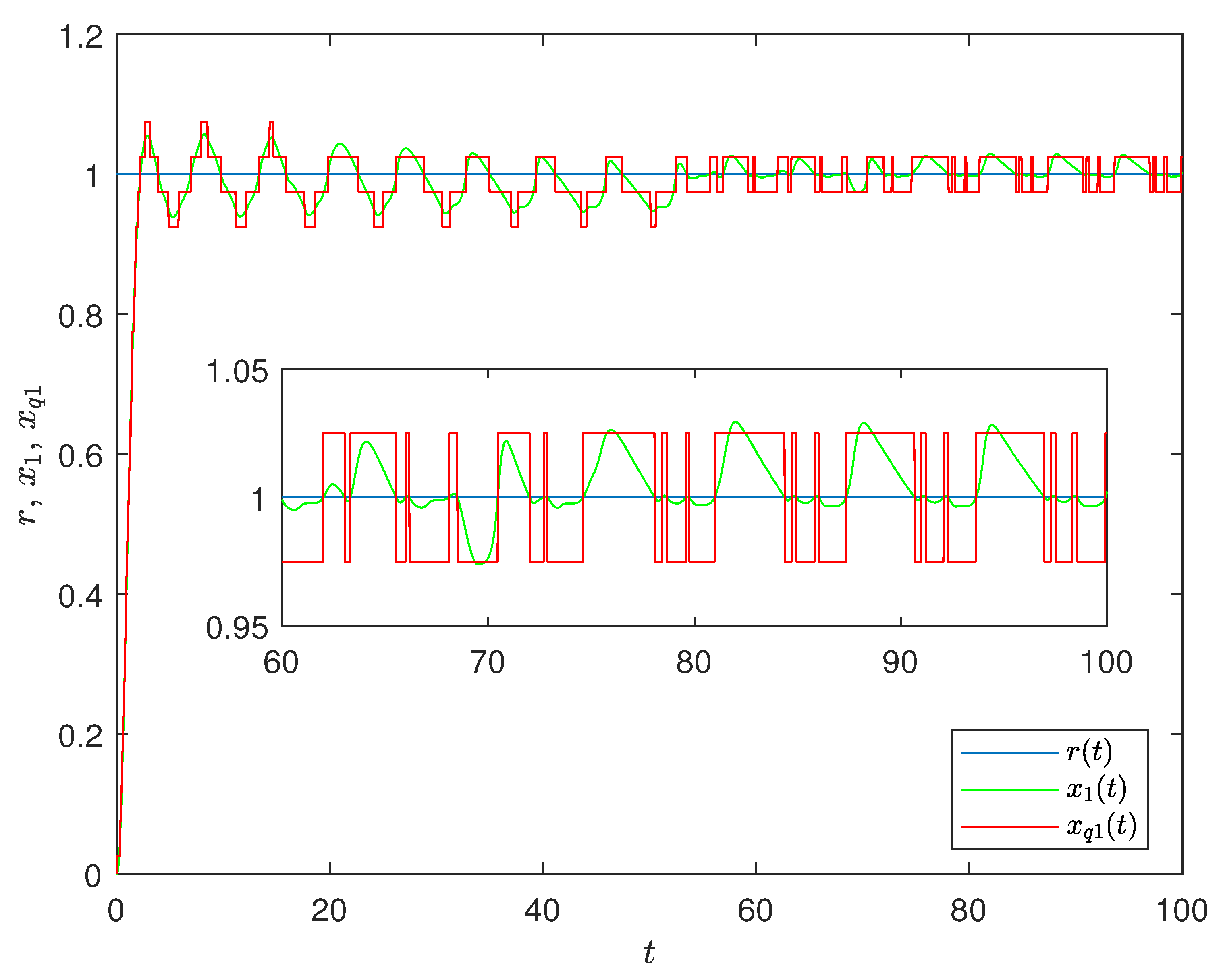
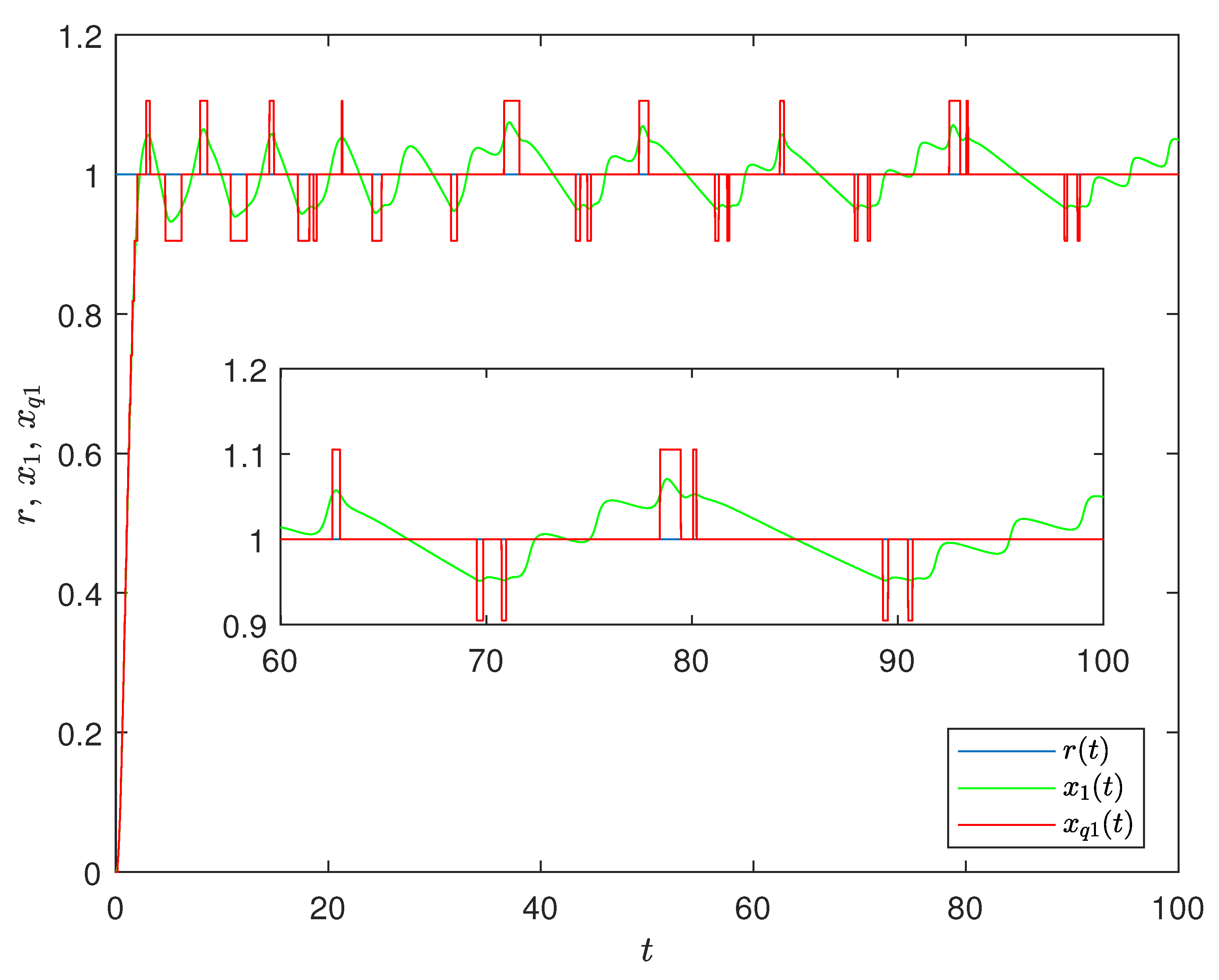
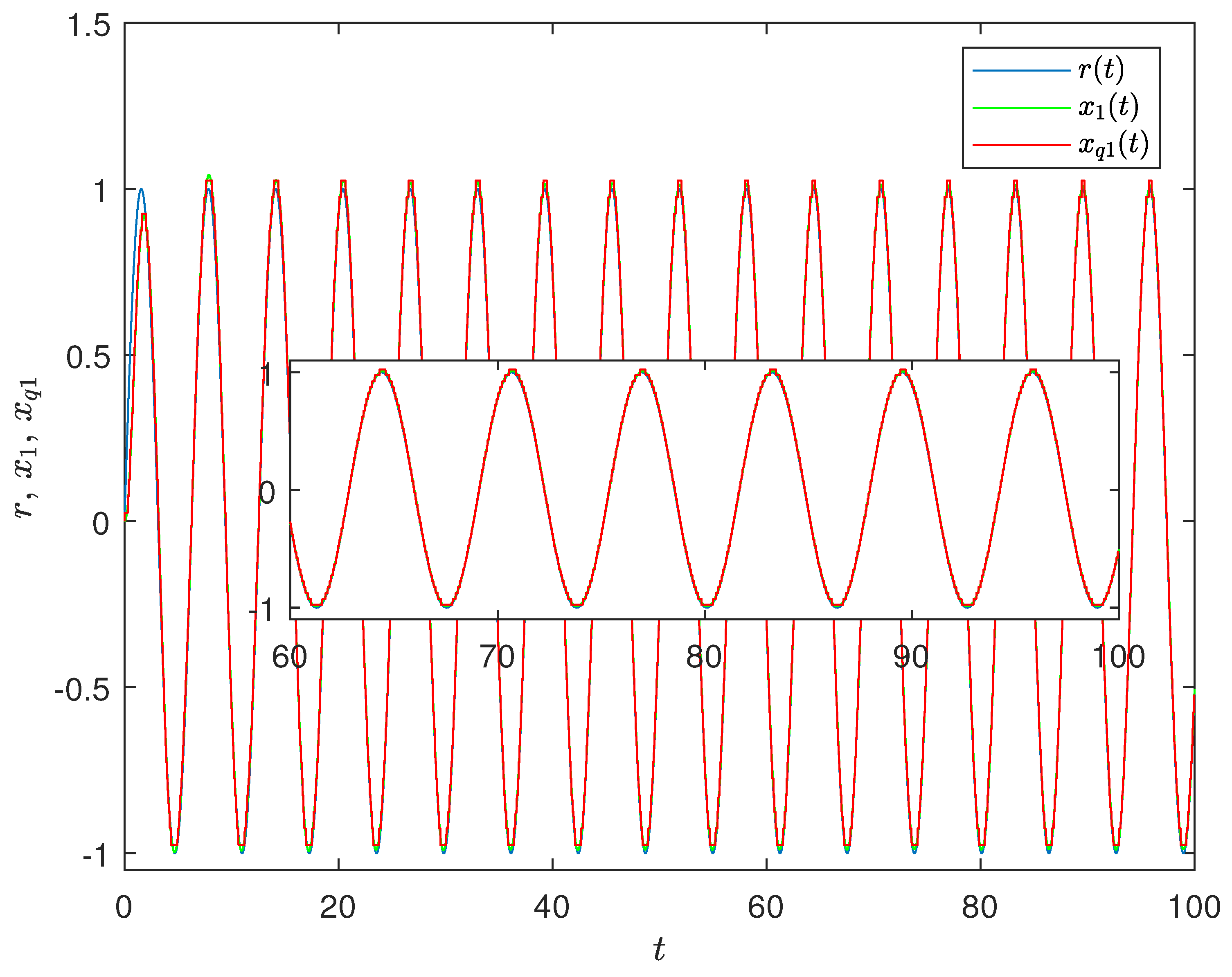
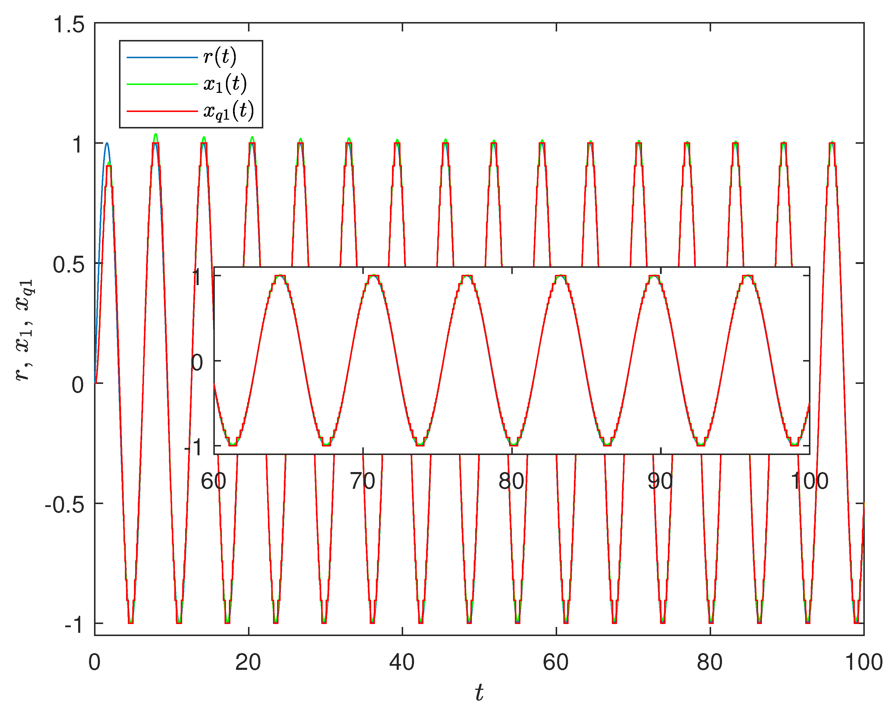
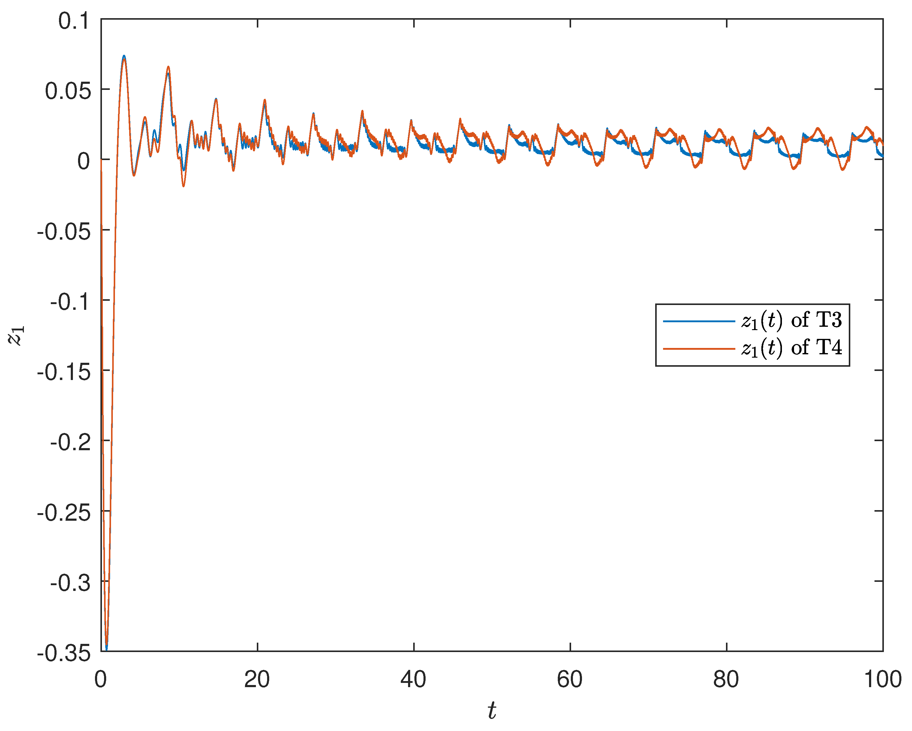
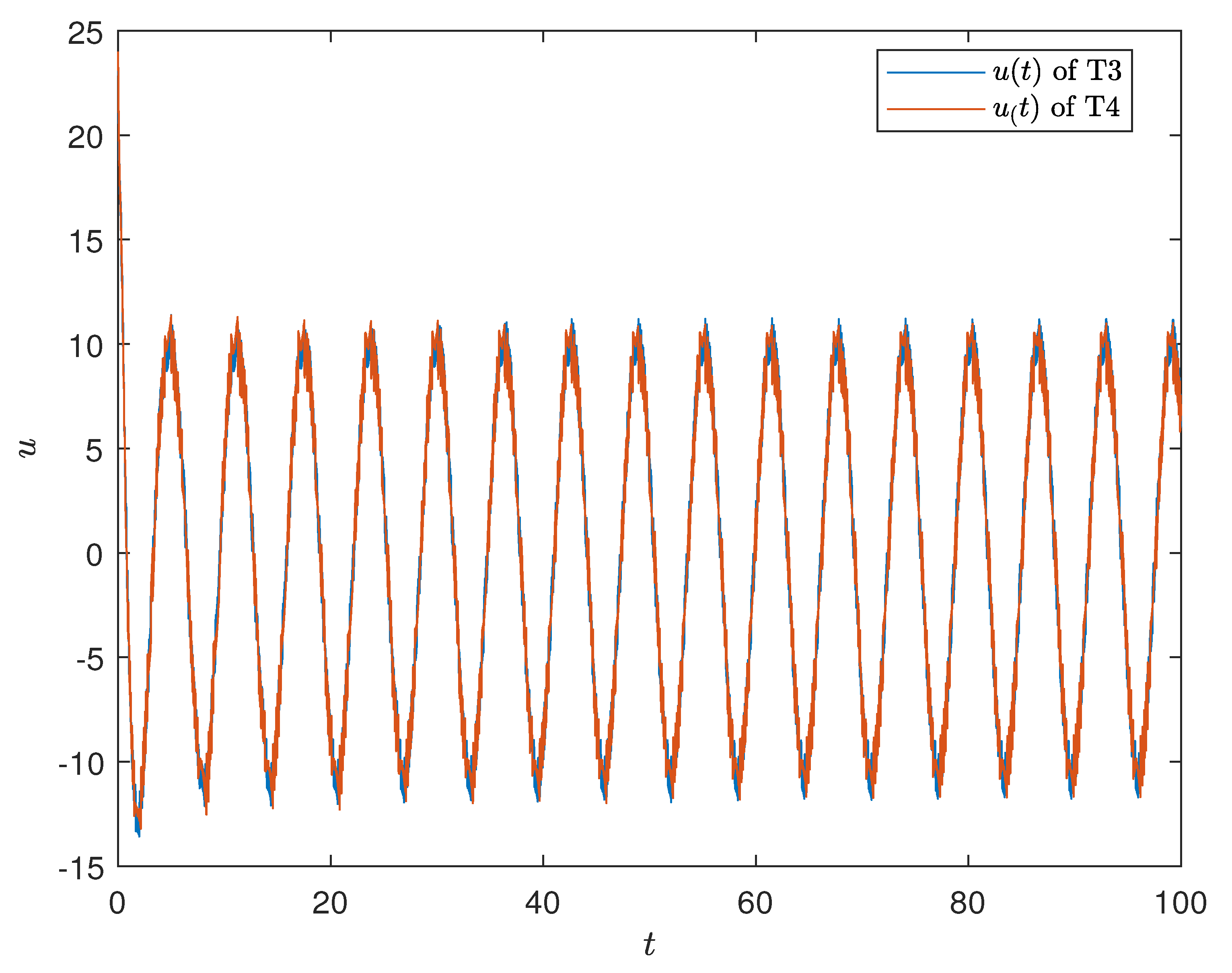
4. Results Validation

In order to verify the theoretical conclusion in Section 3, a contrast experiment is carried out in this section for a three-order nonlinear strict-feedback system under both uncertain parameters and disturbance, which can describe the dynamic of a practical linear-motor-driven gantry system.

$$\left\{\begin{array}{c}{\dot{x}}_1=x_2+D_1(x_1,t)\hfill \\ {\dot{x}}_2=x_3+{\phi }_1^{\top }(\overrightarrow{x})\theta +D_2(x_1,x_2,t)\hfill \\ {\dot{x}}_3=u+{\phi }_2^{\top }(\overrightarrow{x})\theta +D_3(x_1,x_2,x_3,t)\hfill \end{array}\right.$$

(39)

where the states $x_1$, $x_2$ and $x_3$ are the position, velocity and electric current of the system; the input signal u is the voltage applied to the motor; $\theta ={[B,A_f,E,R]}^{\top }$ stands for the vector of unknown parameters; B, $A_f$, E and R represent the viscous coefficient, Coulomb coefficient, inductance factor and resistance, respectively; ${\phi }_1={[-x_2,-arctan(x_2),0,0]}^{\top }$ and ${\phi }_2={[0,0,-x_2,-x_3]}^{\top }$ are known function vectors. To verify the effectiveness of the proposed control approach under strong disturbance, the unknown functions are set as $D_1=d_{1}sin(x_{1}t)$, $D_2=d_2(1-cos(x_1{x}_{2}t))$ and $D_3=d_{3}tanh(x_3)$.

For this simulation, the time interval is $T=0.001$. The parameter settings of the system uncertainties, initial state values, quantizers and control schemes are shown in

Table 1. The settings of the system uncertainties.

	B	${\mathit{A}}_{\mathit{f}}$	E	R	${\mathit{d}}_1$	${\mathit{d}}_2$	${\mathit{d}}_3$
Value	0.15	0.05	0.8	10	0.05	0.02	0.05
Bound	[0.05,0.5]	[0.02,0.5]	[0.2,1]	[1,10]	-	-	-

,

Table 2. The settings of the initial values.

	$\widehat{\mathit{B}}(0)$	${\widehat{\mathit{A}}}_{\mathit{f}}(0)$	$\widehat{\mathit{E}}(0)$	$\widehat{\mathit{R}}(0)$	${\mathit{x}}_1(0)$	${\mathit{x}}_2(0)$	${\mathit{x}}_3(0)$
Value	0.1	0.1	1	5	0	0	0

,

Table 3. The parameter settings of the quantizers.

Uniform quantizer	State quantizer	${\varpi }_{x_1}={\varpi }_{x_2}={\varpi }_{x_3}=0.05$
	Input quantizer	${\varpi }_u=1$
Logarithmic quantizer	State quantizer	${\varpi }_{x_1}={\varpi }_{x_2}={\varpi }_{x_3}=0.01$
		${\delta }_{x_1}={\delta }_{x_2}={\delta }_{x_3}=0.05$
	Input quantizer	${\varpi }_u=1$
		${\delta }_u=0.1$

and

Table 4. The parameter settings of the control scheme.

	Parameter	Value	Parameter	Value
Control law	$k_1$	3	${\epsilon }_1$	0.2
	$k_2$	1	${\epsilon }_2$	0.2
	$k_3$	5	${\epsilon }_3$	0.2
Adaptive law	${\gamma }_1$	0.02	${\epsilon }_{{\theta }_1}$	0.01
	${\gamma }_2$	0.02	${\epsilon }_{{\theta }_2}$	0.01
	${\gamma }_3$	0.02	${\epsilon }_{{\theta }_3}$	0.01
	${\gamma }_4$	5	${\epsilon }_{{\theta }_4}$	0.1

.

In order to test both the stabilization and tracking performance under the designed controller with the uniform and logarithmic quantizer, respectively, the testings in

Table 5. Settings of the testings.

Testings	Quantizer	Trajectory
T1	Uniform quantizer	$r(t)\equiv 1$
T2	Logarithmic quantizer	$r(t)\equiv 1$
T3	Uniform quantizer	$r(t)=sin(t)$
T4	Logarithmic quantizer	$r(t)=sin(t)$

are carried out in this section.

The results of Testings T1–T2 are shown in Figure 4, Figure 5 and Figure 6, which illustrate the tracking performance of Testings T1–T2 and their inputs, respectively. From Figure 4 and Figure 5, the closed-loop system works well and is stable under the designed control approach in spite of strong uncertainties. Moreover, the system responds quickly to the desired steady-state value and converges into a small neighborhood around it whether using uniform quantizers or logarithmic quantizers, which validates the effectiveness of the proposed method on a stabilization mission.

Figure 7, Figure 8, Figure 9 and Figure 10 display the results of Testings T3–T4. Based on Figure 7, Figure 8 and Figure 9, the responses of the system to a sinusoidal signal are all stable regardless of employing uniform quantizers or logarithmic quantizers. In addition, although strong disturbances are applied to the system, the stability of the system is not very affected, and the adaptive laws help the closed-loop system achieve a better performance over time. These results verify the effectiveness of the proposed method on a tracking task.

5. Conclusions

In this article, a class of networked nonlinear systems in strict-feedback form is studied and a quantized backstepping adaptive robust control method, which inherits the advantages of ARC and backstepping methods. In order to analyze the effectiveness of the proposed method, we construct a novel Lyapunov candidate function $V(t)$ which is differentiable and positive definite, although the virtual control law is nondifferentiable. By analyzing the novel positive definite function, the closed-loop system under the designed controller is uniformly ultimate bounded, and the tracking error is related to a pregiven constant and quantization errors. A backstepping ARC scheme is designed for the plant with quantized states and input. The conclusions are also verified by the simulation results. However, some shortcomings of ARC and backstepping methods are also retained, such as the explosion of terms caused by the backstepping method and the nontrue parameter estimation of the ARC law, which lights a path for our future research.

References

1. Tong, S.; Li, Y. Adaptive fuzzy output feedback tracking backstepping control of strict-feedback nonlinear systems with unknown dead zones. IEEE Trans. Fuzzy Syst. 2012, 20, 168–180. [Google Scholar] [CrossRef]
2. Zhang, J.; Sun, W.; Feng, Z. Vehicle yaw stability control via H-infinity gain scheduling. Mech. Syst. Signal Process. 2018, 106, 62–75. [Google Scholar] [CrossRef]
3. Doudou, S.; Khaber, F. Robust adaptive fuzzy control for a class of uncertain nonaffine nonlinear systems with unknown control directions. Trans. Inst. Meas. Control 2021, 43, 01423312211015114. [Google Scholar] [CrossRef]
4. Di Ferdinando, M.; Castillo-Toledo, B.; Di Gennaro, S.; Pepe, P. Robust quantized sampled-data stabilization for a class of lipschitz nonlinear systems with time-varying uncertainties. IEEE Control Syst. Lett. 2021, 6, 1256–1261. [Google Scholar] [CrossRef]
5. Kokotovic, P. The joy of feedback: Nonlinear and adaptive. IEEE Control Syst. 1992, 12, 7–17. [Google Scholar]
6. Lozano, R.; Brogliato, B. Adaptive control of robot manipulators with flexible joints. IEEE Trans. Autom. Control 1992, 37, 174–181. [Google Scholar] [CrossRef]
7. Corless, M.; Leitmann, G. Continuous state feedback guaranteeing uniform ultimate boundedness for uncertain dynamic systems. IEEE Trans. Autom. Control 1981, 26, 1139–1144. [Google Scholar] [CrossRef] [Green Version]
8. Yao, B.; Tomizuka, M. Adaptive robust control of SISO nonlinear systems in a semi-strict feedback form. Automatica 1997, 33, 893–900. [Google Scholar] [CrossRef]
9. Sun, W.; Wang, X.; Zhang, C. A Model-Free Control Strategy for Vehicle Lateral Stability with Adaptive Dynamic Programming. IEEE Trans. Ind. Electron. 2020, 67, 10693–10701. [Google Scholar] [CrossRef]
10. Liu, Y.; Sun, W.; Gao, H. High Precision Robust Control for Periodic Tasks of Linear Motor via B-Spline Wavelet Neural Network Observer. IEEE Trans. Ind. Electron. 2021. [Google Scholar] [CrossRef]
11. Sun, W.; Zhang, Y.; Huang, Y.; Gao, H.; Kaynak, O. Transient-performance-guaranteed robust adaptive control and its application to precision motion control systems. IEEE Trans. Ind. Electron. 2016, 63, 6510–6518. [Google Scholar] [CrossRef]
12. Sun, W.; Liu, Y.; Gao, H. Constrained Sampled-Data ARC for a Class of Cascaded Nonlinear Systems With Applications to Motor-Servo Systems. IEEE Trans. Ind. Informatics 2019, 15, 766–776. [Google Scholar] [CrossRef]
13. Mishra, S.K.; Jha, A.V.; Verma, V.K.; Appasani, B.; Abdelaziz, A.Y.; Bizon, N. An optimized triggering algorithm for event-triggered control of networked control systems. Mathematics 2021, 9, 1262. [Google Scholar] [CrossRef]
14. He, Y.; Ji, M.D.; Zhang, C.K.; Wu, M. Global exponential stability of neural networks with time-varying delay based on free-matrix-based integral inequality. Neural Netw. 2016, 77, 80–86. [Google Scholar] [CrossRef]
15. Nesic, D.; Teel, A. Input-output stability properties of networked control systems. IEEE Trans. Autom. Control 2004, 49, 1650–1667. [Google Scholar] [CrossRef]
16. Wang, Z.; Yang, F.; Ho, D.W.C.; Liu, X. Robust H Control for Networked Systems With Random Packet Losses. IEEE Trans. Syst. Man Cybern. Part B 2007, 37, 916–924. [Google Scholar] [CrossRef] [PubMed]
17. Quevedo, D.E.; Nesic, D. Input-to-state stability of packetized predictive control over unreliable networks affected by packet-dropouts. IEEE Trans. Autom. Control 2011, 56, 370–375. [Google Scholar] [CrossRef] [Green Version]
18. Zhao, Y.; Liu, G.; Rees, D. Actively compensating for data packet disorder in networked control systems. IEEE Trans. Circuits Syst. 2010, 57, 913–917. [Google Scholar] [CrossRef]
19. Gao, H.; Chen, T. A new approach to quantized feedback control systems. Automatica 2008, 44, 534–542. [Google Scholar] [CrossRef]
20. Chen, W.; Jiao, L.; Li, J.; Li, R. Adaptive NN Backstepping Output-Feedback Control for Stochastic Nonlinear Strict-Feedback Systems With Time-Varying Delays. IEEE Trans. Syst. Man Cybern. Part B 2010, 40, 939–950. [Google Scholar] [CrossRef]
21. Zhang, J.; Xu, H.; Zheng, H. Adaptive sampled-data output tracking of parametric strict-feedback non-linear systems. IET Control Theory Appl. 2012, 6, 985–991. [Google Scholar] [CrossRef]
22. Zeng, D.; Liu, Z.; Chen, C.L.; Zhang, Y. Adaptive neural tracking control for switched nonlinear systems with state quantization. Neurocomputing 2021, 454, 392–404. [Google Scholar] [CrossRef]
23. Zhou, J.; Wen, C.; Wang, W.; Yang, F. Adaptive Backstepping Control of Nonlinear Uncertain Systems with Quantized States. IEEE Trans. Autom. Control 2019, 64, 4756–4763. [Google Scholar] [CrossRef]
24. Aslmostafa, E.; Ghaemi, S.; Badamchizadeh, M.A.; Ghiasi, A.R. Adaptive backstepping quantized control for a class of unknown nonlinear systems. ISA Trans. 2021. [Google Scholar] [CrossRef]
25. Sun, H.; Hovakimyan, N.; Basar, T. L1 adaptive controller for uncertain nonlinear multi-input multi-output systems with input quantization. IEEE Trans. Autom. Control 2012, 57, 565–578. [Google Scholar] [CrossRef]
26. Zhou, J.; Wen, C.; Yang, G. Adaptive backsepping stabilization of nonlinear uncertain systems with quantized input signal. IEEE Trans. Autom. Control 2014, 59, 460–464. [Google Scholar] [CrossRef]
27. Xing, L.; Wen, C.; Zhu, Y.; Su, H.; Liu, Z. Output feedback control for uncertain nonlinear systems with input quantization. Automatica 2016, 65, 191–202. [Google Scholar] [CrossRef]
28. Liu, T.; Jiang, Z.; Hill, D. A sector bound approach to feedback control of nonlinear systems with state quantization. Automatica 2012, 48, 145–152. [Google Scholar] [CrossRef]
29. Ceragioli, F.; De Persis, C.; Frasca, P. Discontinuities and Hystersis in Quantized Average Consensus. Automatica 2011, 47, 1919–1928. [Google Scholar] [CrossRef] [Green Version]
Figure 1. The signal transmission in networked control systems.
Electronics 10 02783 g001
Figure 2. Diagram of the uniform quantization.
Electronics 10 02783 g002
Figure 3. Diagram of the logarithmic quantization.
Electronics 10 02783 g003
Figure 4. x 1 and x q 1 of Testings T1.
Electronics 10 02783 g004
Figure 5. x 1 and x q 1 of Testings T2.
Electronics 10 02783 g005
Figure 6. The input signals of Testings T1–T2.
Electronics 10 02783 g006
Figure 7. x 1 and x q 1 of Testings T3.
Electronics 10 02783 g007
Figure 8. x 1 and x q 1 of Testings T4.
Electronics 10 02783 g008
Figure 9. The errors z 1 of Testings T3–T4.
Electronics 10 02783 g009
Figure 10. The input signals of Testings T3–T4.
Electronics 10 02783 g010