Abstract
The identification of actual photovoltaic (PV) model parameters under real operating condition is a crucial step for PV engineering. An accurate and trusted model depends mainly on the accuracy of the model parameters. In this paper, an accurate and enhanced methodology is intended for PV module parameters extraction in outdoor conditions. The proposed methodology combines numerical methods and analytical formulations of the one diode model to derive the five unknown parameters in any operating condition of irradiance and temperature. First, the measured I-V curves at a random weather condition are translated to standard test conditions (i.e., G = 1000 W/m2, T = 25 °C), using translation equations. The second step consists of using an optimization algorithm namely the moth flame algorithm (MFO) to find out the five parameters at standard test conditions. Analytical formulations, at a random irradiance and temperature, are then used to express the unknown parameters at any irradiance and temperature. The proposed approach is validated under outdoor conditions against measured I-V curves at different irradiances and temperatures. The validation has also been performed under dynamic operation where the measured maximum power point coordinates (MPP) are compared to the predicted maximum power points. The obtained results from the adopted hybrid methodology confirm the accuracy of the parameter extraction procedure.
1. Introduction
Photovoltaic module is the critical element in a photovoltaic array that is responsible for converting solar energy into usable electrical power. Several studies have reported the electrical modeling of PV modules due to their prime involvement in predicting the overall performance of photovoltaic systems in real working conditions and analyze its efficiency before they are fully employed [1]. This modeling is also important in many applications, which include the maximum power exploitation [2], fault detection and diagnosis [3,4], module degradation analysis [5], and power management of an existing PV power plant [6]. In most related literature, the one diode model has been extensively used due to its simplicity, usefulness and accurate simulation of actual PV plants [7,8]. The modeling of the photovoltaic module is closely related to its intrinsic properties and the five parameters which are included in its mathematical model [9]. From this point of view, it becomes clear the importance of an accurate parameters extraction.
Most of the existing literature that covers PV module parameters extraction explores two main approaches namely analytical and numerical methods. Analytical methods focus on the physical relationship between extrinsic and intrinsic variables while the basic goal of numerical methods is to minimize the quadratic error between measured and estimated variables of interest. For instance, De Soto et al., used an analytical approach based totally on the current-voltage equation analysis at three key points, namely: short circuit point (Isc), open circuit point (Voc) and the coordinates of the maximum power point Pm (Im, Vm). These points are formulated in analytical equations where the five unknown parameters can be extracted using iterative approach [10]. In other work proposed in [11], the matching between experimental and theoretical I-V curves is performed by solving the analytic equations, and an iterative variation of Rs and Rp. It is worth mentioning that in many analytical methods, to avoid calculation burden, one of the unknown parameters is fixed and the remainders are found by simultaneous equations solution. For instance, the work proposed in [12] implements an analytical approach that involves reformulating voltage and current equations in a way that enables them to analytically evaluate the five parameters, relying only on the manufacturers’ datasheets. Compared to the simultaneous solution for nonlinear equations, this approach offers appropriate outcomes. In reference [13], the authors have used an analytical method, where the electrical circuit parameters are extracted by solving nonlinear equations primarily based on data provided by manufacturers under standard conditions. A simple technique was suggested in reference [14] in which three parameters are specified: ideality factor, Rs, and Rsh, and it needs four inputs from the manufacturer’s data, specifically: Voc, Isc, Impp and Vmpp. This method has given good results on crystalline silicon cells. It should be noted that the trend towards simple analytical models by the researcher community that rely primarily on fixing certain parameters or assigning them random values to decrease the calculation burden can be less precise and cause simulation errors.
Numerical methods and optimization algorithms inspired by nature behavior can bypass analytical methods’ complexity and avoid falling into local minima/maxima solutions. Several numerical algorithms, dedicated to the extraction of a single diode model electrical parameters, have been proposed in the literature during the last decade. For instance, in [15], the proposed approach involves the use of genetic algorithms (GAs) to find the five unknown parameters. In [16], particle swarm optimization (PSO) is used to extract the PV module electrical parameters, this is done with inverse barrier constraint. To overcome the difficulties in the DE approach, [17] proposes an improved adaptive differential algorithm (IADE) to extract parameters from a single diode model. Reference [18] proposed artificial bee swarm optimization (ABSO), while [19] suggested the artificial bee colony (ABC). In reference [20], teaching learning-based optimization algorithm (TLBO) was successfully applied to identify parameters for four different types of cells: dye-sensitized solar cells (DSSC), plastic solar cell, and silicon solar cell, as well as silicon solar modules [21] suggested bird mating optimizer approach (SBMO). The flower pollination algorithm (FPA) was suggested by [22]. Reference [23] proposed an improved cuckoo search algorithm (ImCSA). In [24], the generalized oppositional teaching learning-based optimization (GOTLBO) algorithm is utilized to extract parameters for PV module. [25] also estimated parameters in the silicon cell, by making extensive use of ant lion optimization (ALO).
It can be noted that the above numerical techniques are primarily based especially on the measured data under different environmental conditions (irradiance, temperature) to extract the parameters. Indeed, most of these parameter extraction algorithms use measured I-V curve data and try to find a unique parameters vector that minimizes the difference between measured and predicted current without taking into account the working conditions including irradiance and temperature. However, most of PV cell parameters are sensitive to weather conditions, so supposing them constant is not quite accurate.
The main motivation of the present paper is to propose an accurate module parameters extraction approach that combines analytical formulation and a numerical optimization method. The suggested approach contains three primary stages. In the first stage, actual I-V curves translation to the reference conditions (i.e., G = 1000 W/m2, T = 25 °C) using analytical formulation. In the second stage, the five unknown parameters in standard conditions are extracted based on the moth flame optimization (MFO) algorithm combining the translated I-V curves with the analytical formula at the reference conditions. The last step consists to find out the I-V couples at actual conditions of temperature and irradiance based on analytical formulas and the reference parameters extracted numerically by the MFO algorithm.
The remaining parts of this paper are summarized in the following points: Section 2, explains the modeling of the PV array and the proposed parameters extraction approach. The MFO algorithm and five-parameter model are also presented. Section 3 deals with the presentation of the grid-connected PV system used in this study and provides the experimental results and evaluation of the proposed approach. Finally, this research is concluded in the last section.
2. Modeling of a PV Array and Parameters Identification
2.1. Modeling of a PV Array
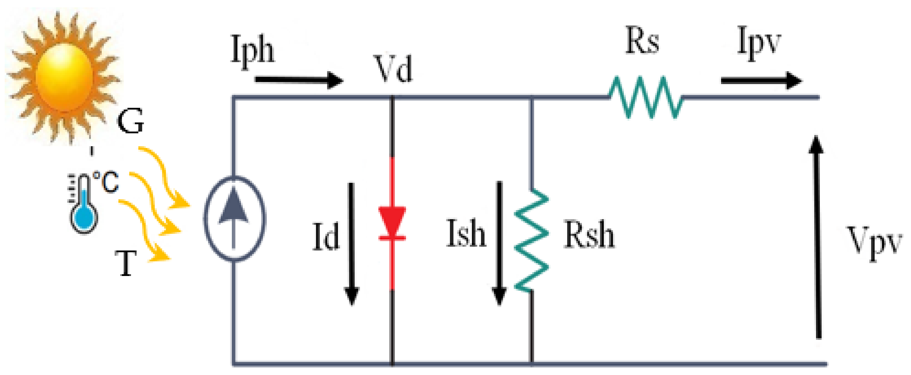
A photovoltaic module is a collection of solar cells that are connected both serially and parallelly, which produce electrical energy when exposed to light by a mechanism that converts the solar radiation absorbed into electricity [26]. It is an established fact that photovoltaic cell modeling is necessary to understand their behavior under different operating temperatures and irradiance conditions. Model of one diode (ODM) [27,28], shown in Figure 1 is the most commonly used model in the literature. Iph, Io, n, Rs, and Rsh are the five unknown parameters in this model that must be calculated. It is worth mentioning here that some manufacturers don’t include these parameters on their datasheets.

Figure 1.
Equivalent circuit representing the ODM of the pv cell.
The following nonlinear equation gives the voltage-current relationship of a PV cell [3,29]:
where Iph is the photo-current in (A), Io is the diode saturation current in (A), n is the ideality factor of the diode, Rs and Rsh are the series and the shunt resistances respectively in (Ω), T is the temperature of the PN junction in Kelvin, kB is the Boltzmann constant (1.38 × 10⁻²³ J K−1), and q is the electron charge (1.602 × 10⁻¹⁹ C).
2.2. Current-Voltage Translation to Reference Conditions
In outdoor operating conditions, it is almost impossible to reach, at the same time, standard conditions (i.e., Gref = 1000 W/m2, Tref = 25 °C). Therefore, an efficient mathematical analytical method that translates arbitrary I-V curves taken at any other temperature and irradiance than 1000 W/m2 and 25 °C can be used to obtain reference curves [30]. The expressions given in Equations (2) and (3) are used to translate the short circuit current and the open-circuit voltage at their reference values Isc,ref and Voc,ref, respectively:
where α is the current temperature coefficient, β is the voltage temperature coefficient, their value is shown in Table 1, n is the modified ideality factor which is taken equal to the value given by the manufacturer, Gmeas and Gref are measured and reference irradiance in W/m2 respectively, Tmeas and Tref are measured and reference temperature in °C.

Table 1.
Isofoton “106 W-12 V” PV module specification.
The following mathematical expressions translate every point on the measured curve (Vmeas, Imeas) to the expected point on the translated reference curve (Vref, Iref):
where ΔIsc and ΔVoc are calculated by the following relations:
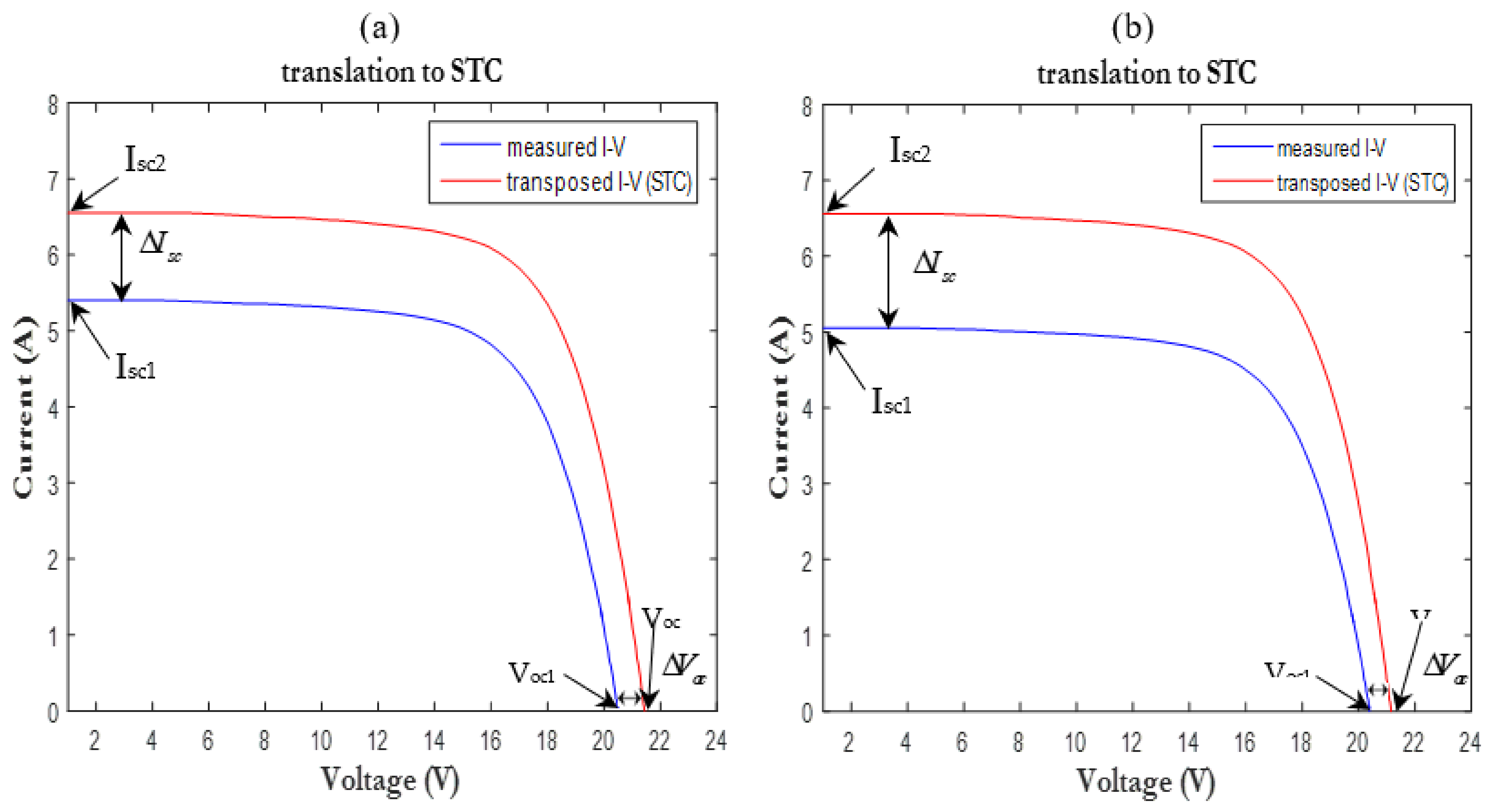
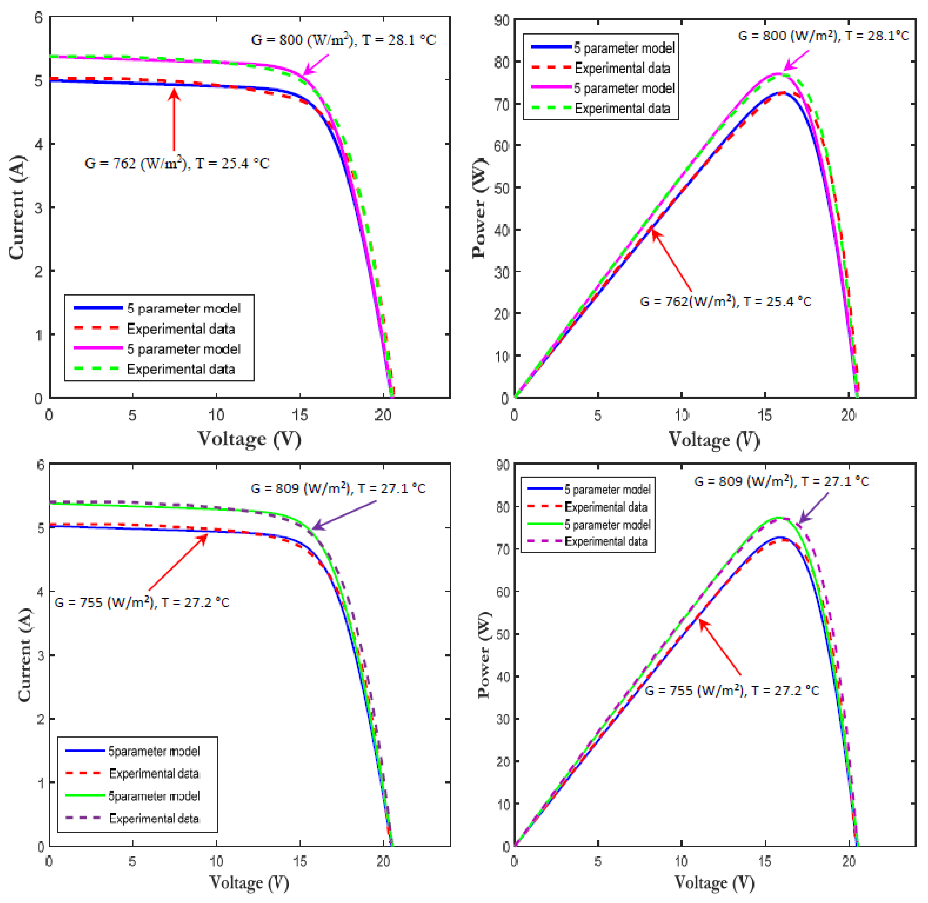
For instance, Figure 2 gives the translated curves from a measured I-V curves at (Gmeas = 755 W/m2, Tmeas = 27.2 °C) and (Gmeas = 809 W/m2, Tmeas = 27.1 °C).
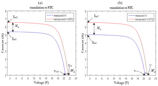
Figure 2.
Measured and translated I-V curve to reference condition (Gref = 1000 W/m2, Tref = 25 °C) at (a) (Gmeas = 809 W/m2, Tmeas = 27.1 °C), (b) (Gmeas = 755 W/m2, Tmeas = 27.2 °C) for ISOFOTON 106 PV module.
We notice that almost all the proposed numerical algorithms found in the literature give a unique parameters vector that does not correlate with the weather condition changes. The parameters found based on these algorithms are not quite accurate given that some parameters are temperature or irradiance sensitive.
2.3. Identification of Reference Parameters
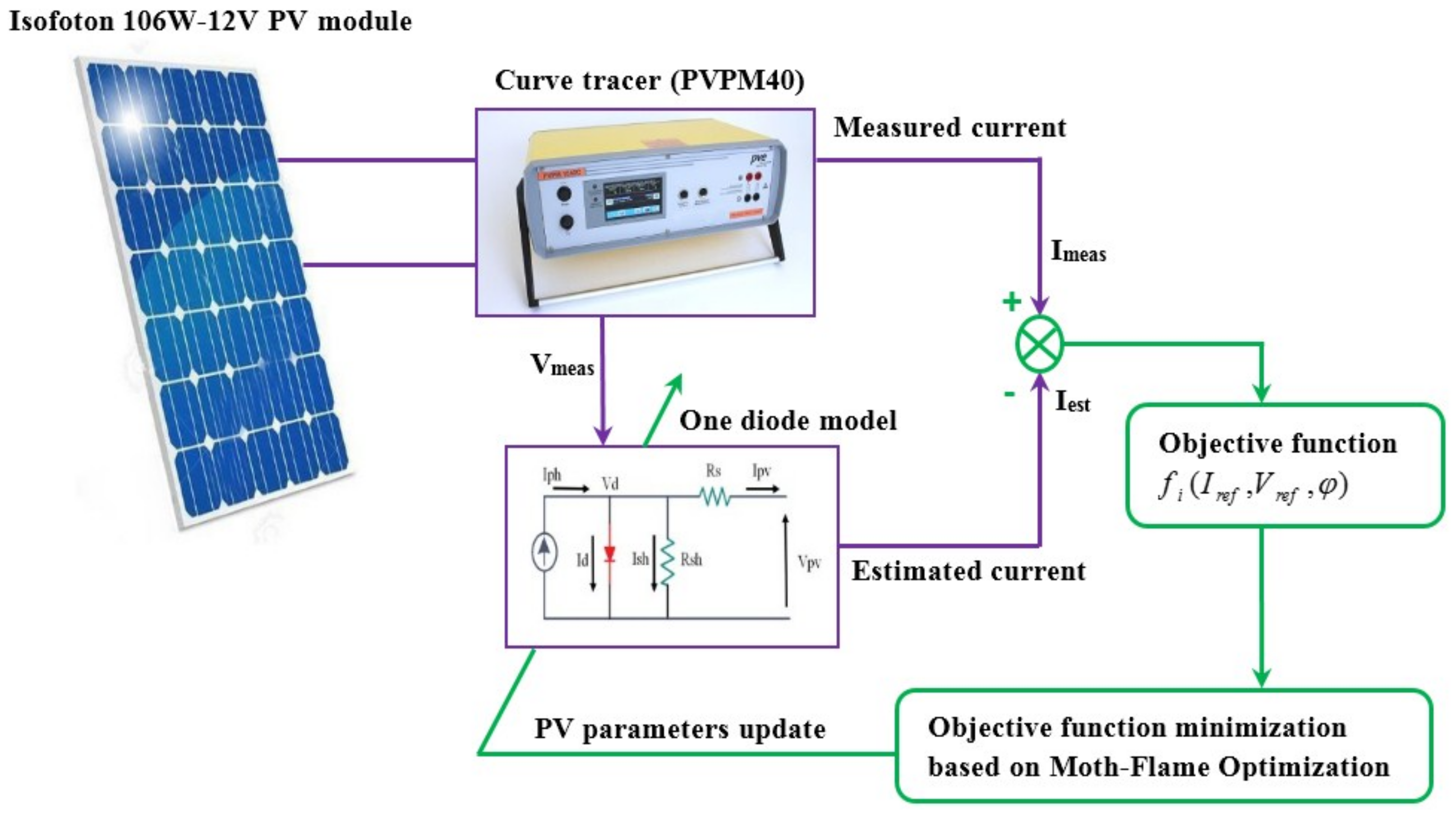
After obtaining the reference curve data from the translation process, explained in the previous section, the five unknown parameters at the reference condition can be extracted using meta-heuristic algorithms. In this study, the moth-flame optimization (MFO) algorithm, suggested by Mirjalili in 2015 [31], is chosen for this task. The basic idea of this parameters extraction concept is represented in Figure 3. The objective is to minimize the root-mean-square error (RMSE) between Iref and Iest, as given in Equation (8) where the calculated and estimated current reference values are involved [32]:
where:
where S is the number of data points. The reference current and voltage of the PV module obtained from the translated I-V curves are Iref and Vref, and φ = [Iph,ref, Io,ref, nref, Rs,ref and Rsh,ref] represents the vector of the five unknowns electrical parameters in the reference condition.

Figure 3.
Flowchart for the identification of PV reference parameters based on Moth-Flame Optimization (MFO).
2.4. PV Module Parameter Extraction Based on the MFO Algorithm
The problem of extracting the five unknown parameters in a single diode model is treated as an optimization problem based on the MFO algorithm described in reference [31]. The description and the details of using this algorithm for PV module parameter extraction purposes is given below:
In the first step, the N values of the couples (Vref and Iref) obtained by translation equations are loaded to MFO algorithm and the five parameters of single diode model are converted to vectors in order to emulate moth positions. The elements of the moths scattered in the search space are randomly initialized based on the number of search agents (moths) and the number of variables (dimensions). The number of parameters (Iph, Io, n, Rs and Rsh) in the one diode model determine the dimensions (d) of the search space where moths moves in. The random initial solutions are generated using the I function given by the following expression [31]:
In the second step, a moth updates its position at each iteration using the objective function (RMSE) as defined in Equation (8) and Vref, Iref.
In the third step, the number of flames is updated using Equation (11) given below [31]:
The fitness value is calculated at each iteration with updating the distance between the moth and the flame as described in Algorithm 1.
| Algorithm 1: Moth flame optimization (MFO) for pv module parameters extraction |
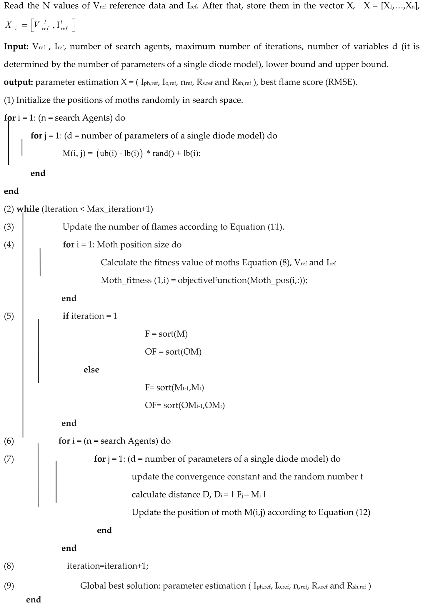 |
Each moth position is updated with respect to the flame using [31]:
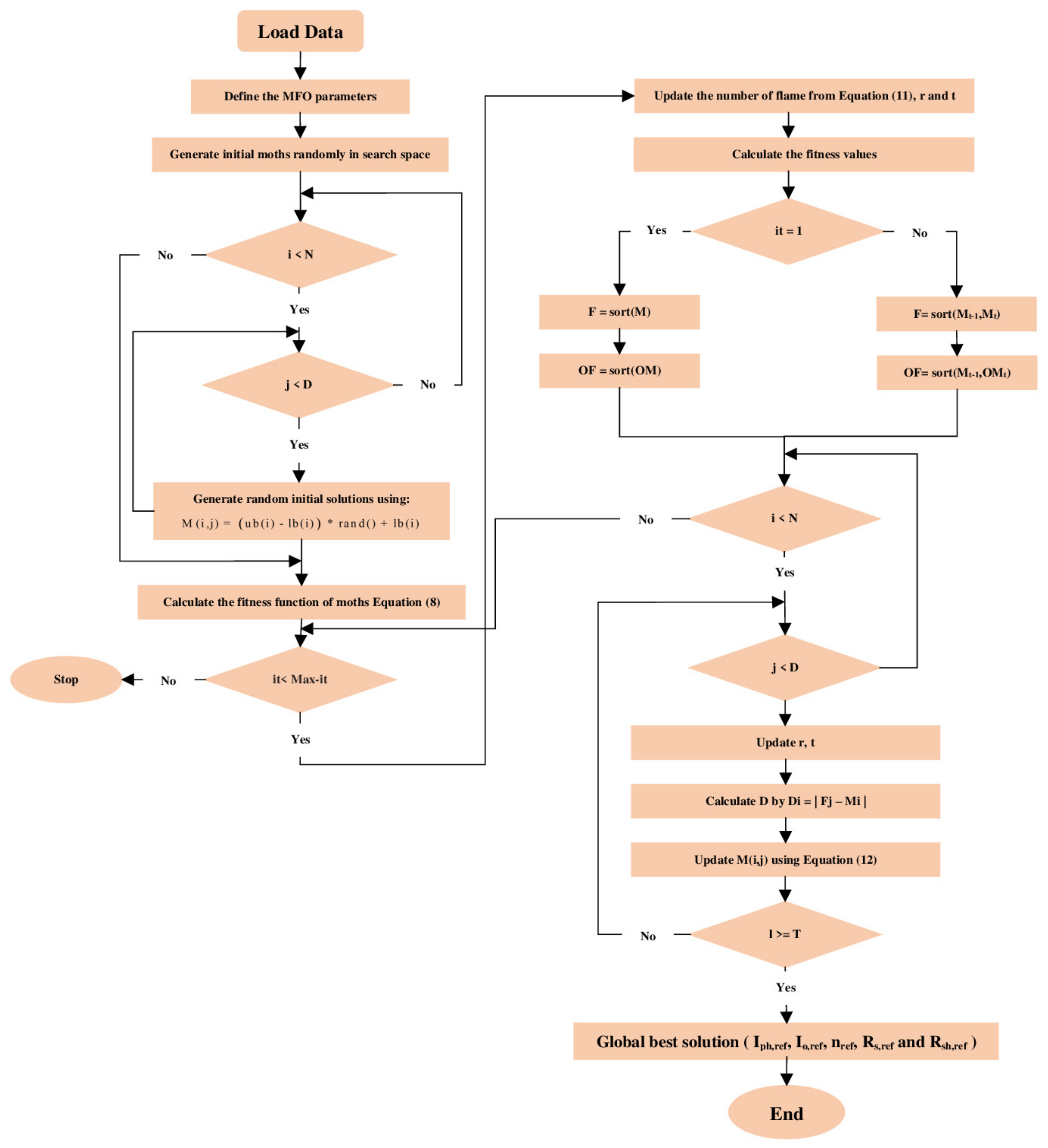
The goal of the optimization is to minimize the error function fi (Iref, Vref, φ), expressed in Equation (9), which represents the difference between the reference and estimated currents. Finally the most appropriate final solution vector X = (Iph,ref, Io,ref, nref, Rs,ref and Rsh,ref), is selected according to the minimum value of the fitness function. The flowchart of MFO algorithm used for parameter extraction of pv module is given in Figure 4.

Figure 4.
Flowchart of moth-flame optimization algorithm for parameter extraction.
2.5. Five-Parameters under Actual Operating Conditions
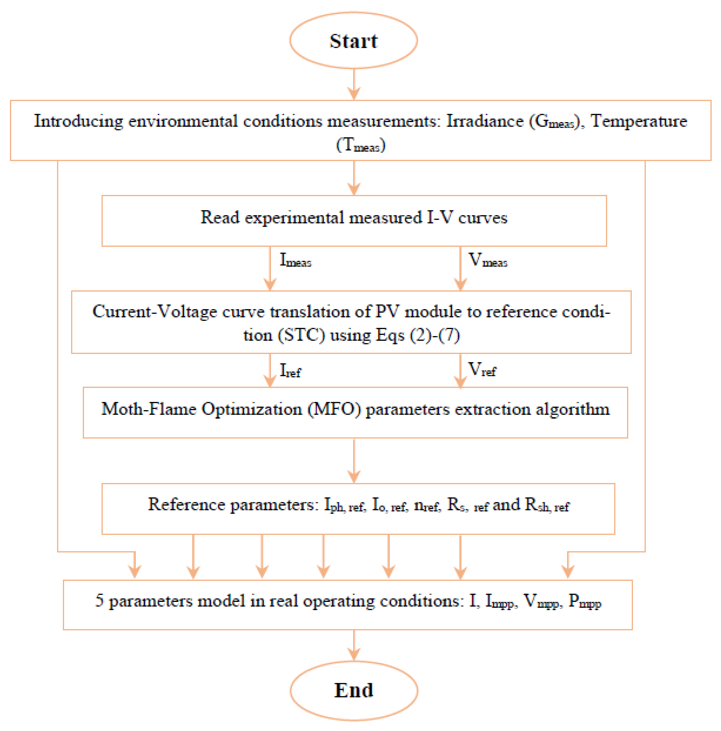
The remaining step consists to find out the I-V couples at actual conditions of temperature and solar irradiance, based on fully analytical formulas and reference parameters extracted by MFO algorithm. The analytical formulas allowing to find the five parameters as a function of temperature and irradiance are given by Equations (13)–(18) [33,34,35]. The details of the proposed approach is summarized by the flowchart shown in Figure 5.
where Iph, Io, n, Rs and Rsh are the five parameters at actual operating conditions, while the Iph,ref, Io,ref, nref, Rs,ref and Rsh,ref are the five unknown parameters at the reference conditions, Eg is the bandgap energy of the semiconductor, Eg,ref is the bandgap energy for reference conditions.
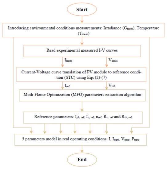
Figure 5.
Flowchart of parameters extraction of a PV module using the proposed procedure.
3. Experimental Results and Validation
3.1. Grid-Connected PV System Description
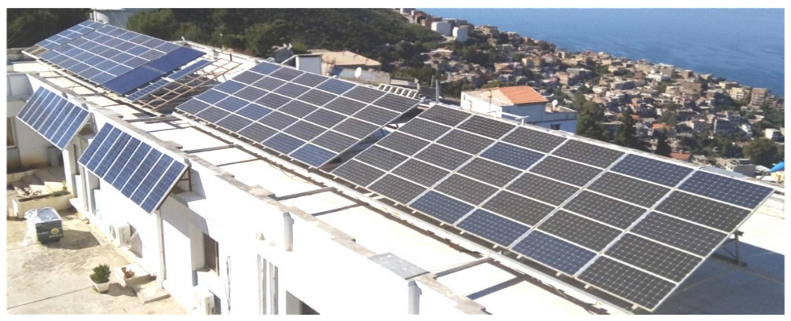
The experimental grid-connected PV system shown in Figure 6 is taken as a platform to validate the proposed parameters extractions procedure. This solar power plant consists of 90 PV modules producing 9.54 kWp of 125–450 V as DC voltage and 220 V as AC voltage. This is an array consisting of three identical PV sub-arrays producing 3.18 kW each, and each one is connected to a 2.5 kW single-phase PV inverter (IG30 from Fronius Company, Denver, CO, USA). Each sub-array contains thirteen 106 W-12 V PV modules installed in two parallel strings of 15 modules each.
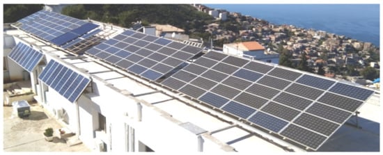
Figure 6.
Grid connected PV system, installed at CDER in Algiers, Algeria.
The electrical characteristics of the PV module are given in Table 1.
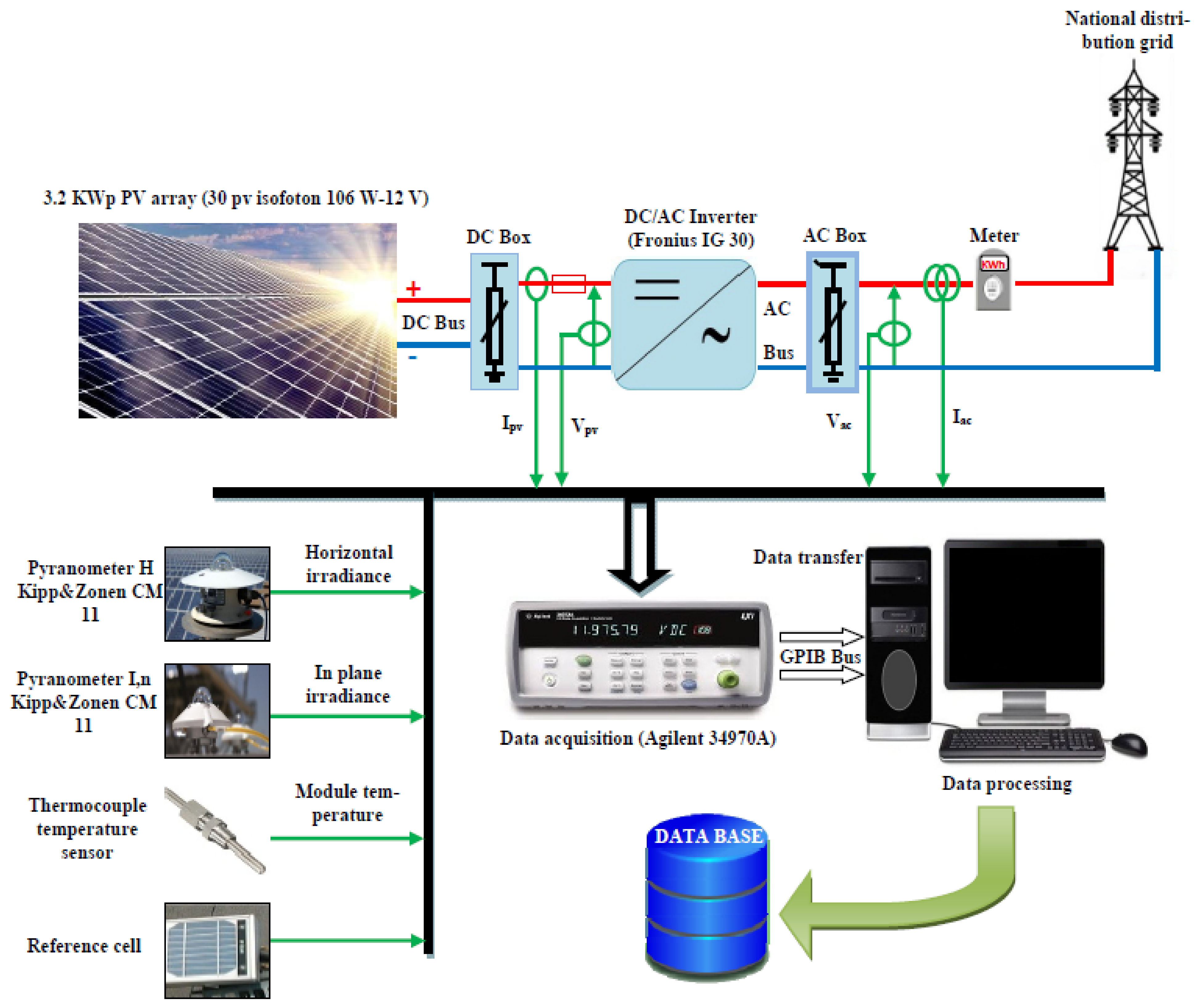
Voltage and current data for the MPP coordinates, solar radiation and temperature are collected every 1 min according to which 1440 samples are collected daily. Figure 7 shows the grid-connected PV system that was employed in this study for monitoring.

Figure 7.
Scheme of the monitoring grid connected PV system used in this study.
3.2. Reference Parameters Extraction Results
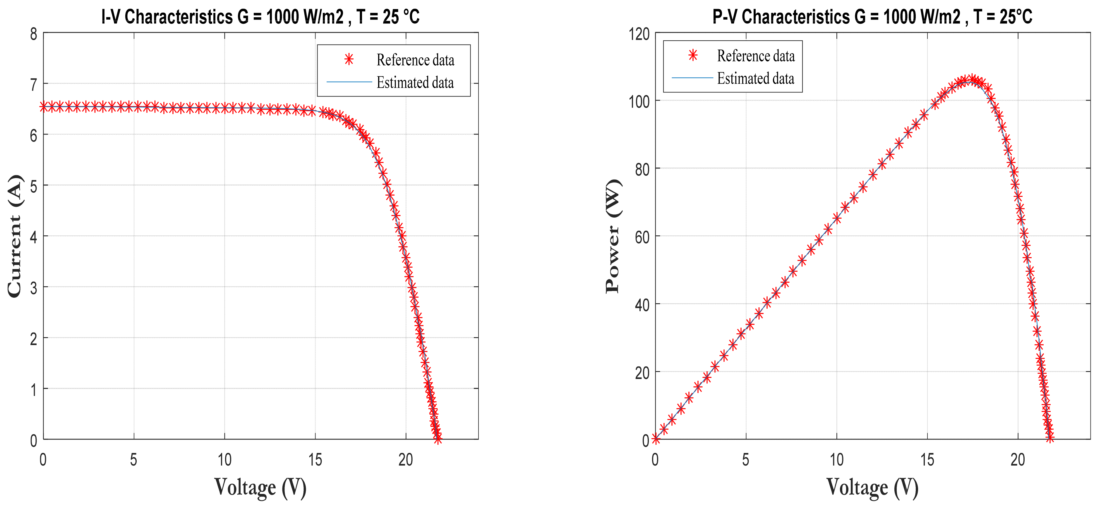
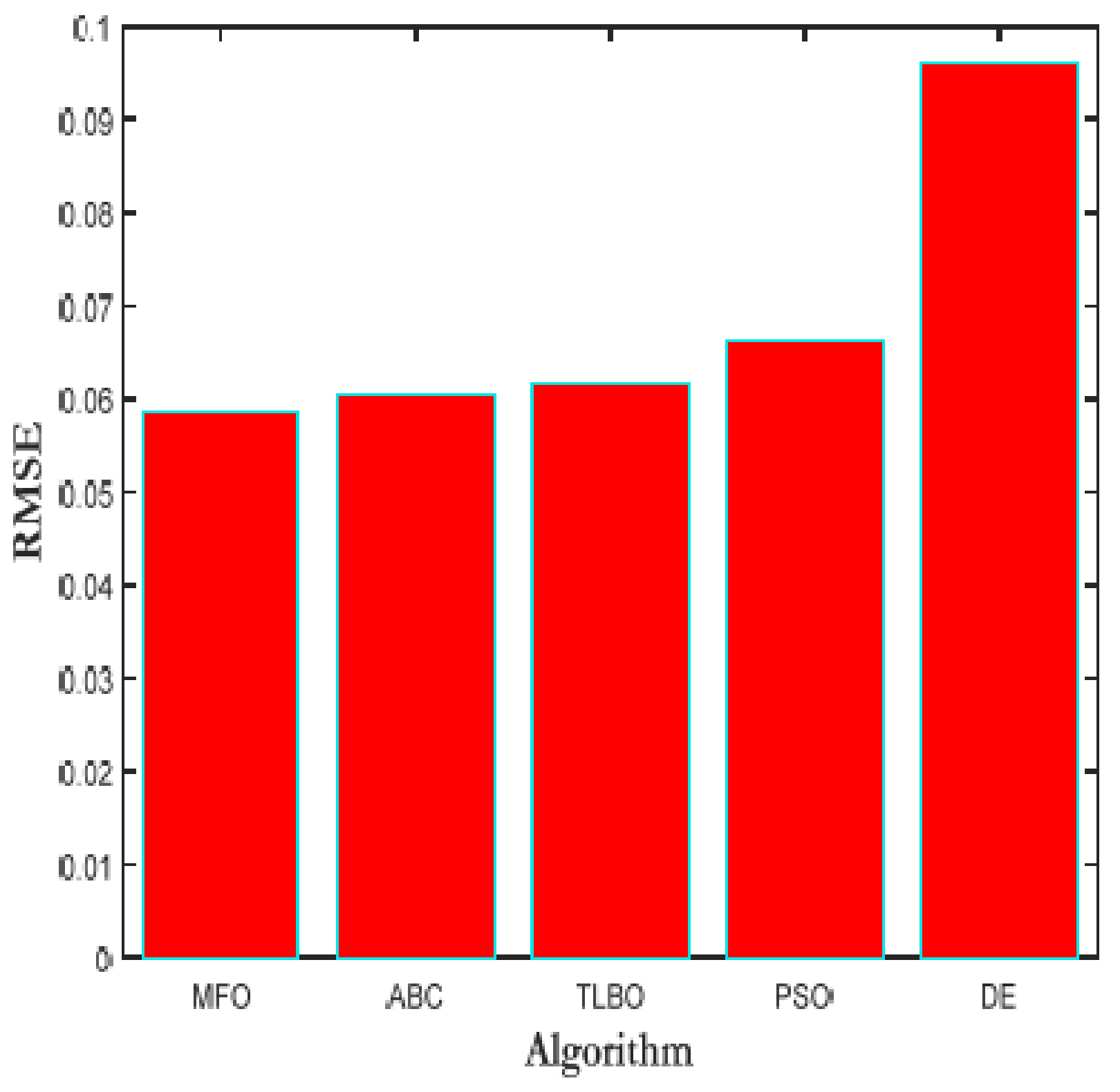
The effectiveness of PV module reference parameters extraction based on MFO algorithm is validated in the MATLAB/SIMULINK environment (From Mathworks Company). The MFO is used to estimate the unknown ODM parameters using the data obtained from the analytical translation method. Table 2 shows the five reference parameters of an Isofoton 106 W-12 V PV module (From Isofoton Company) obtained using the MFO algorithm. Figure 8 highlights the I-V curve obtained by the translation process and the estimated one where a good fit is obtained. Furthermore, the proposed algorithm is compared with four algorithms: ABC [36], PSO [37], DE [38], and TLBO [39]. This comparison is based on the reference data received through the analytical current-voltage translation procedure. The results of this comparative study are given in Table 3 in terms of the objective function values. Based on these results, it can be noticed that the best RMSE value (0.058483) is obtained using the MFO optimization algorithm (see Figure 9).
Table 2.
Parameters extracted using the MFO algorithm from the “isofoton 106 W-12 V” solar PV module.
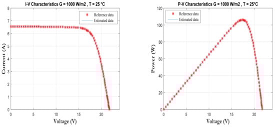
Figure 8.
Comparison between the estimated data with MFO and reference data obtained from the translation method of the I-V and P-V curves at (G = 1000 W/m2 and T = 25 °C).
Table 3.
Objective function values obtained by different algorithms.

Figure 9.
RMSE for different algorithms at reference data “G = 1000 W/m2 and T = 25 °C”.
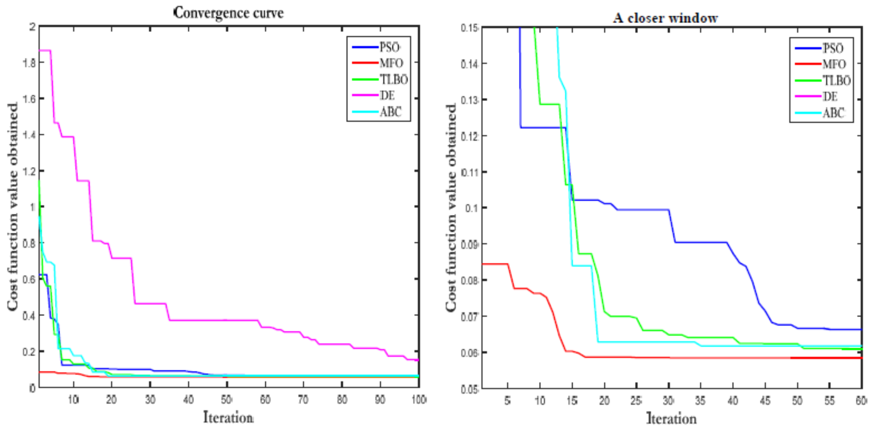
The convergence speeds of the four optimization algorithms are illustrated in Figure 10. From this figure, the MFO shows an impressive affinity speed where the convergence is reached after only 25 iterations, unlike the other algorithms that require a lot of convergence time.
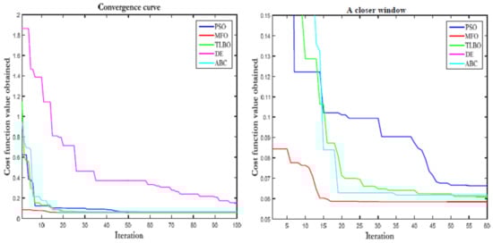
Figure 10.
Convergence curves for different optimization algorithms.
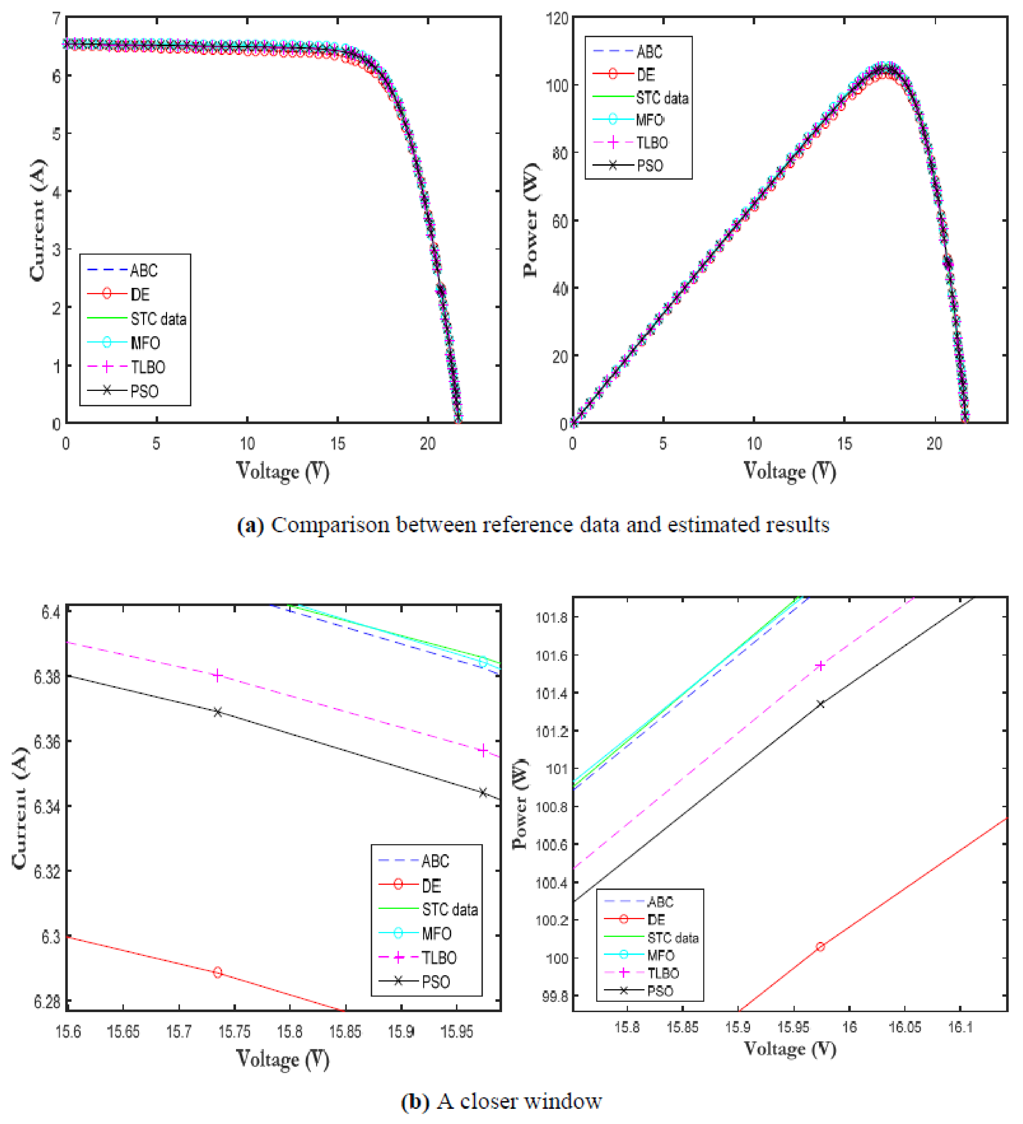
Figure 11 depicts the I-V and P-V characteristics obtained by the four optimization algorithms. It is clearly shown, in the zoomed Figure 11b, that the results obtained from the proposed algorithm are very close to the figure given by reference data under standard conditions. This result reveals that MFO algorithm is good in terms of convergence speed to an optimal solution. Furthermore, its simplicity in terms of implementation makes it highly competitive in determining the PV model parameters with high accuracy.
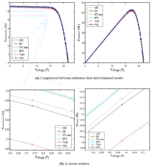
Figure 11.
(a) Comparison between reference data obtained from the translation method (STC data) and estimated results for each algorithm: I-V and P-V curves at “G = 1000 W/m2, T = 25°C”, (b) the zoom of the subfigure (a).
3.3. Accuracy of the Proposed Methodology
To check the precision of the calculated parameters to obtain the estimated I-V couples at random irradiance and temperature, a comparison between experimental I-V and P-V curves and the estimated one is performed as shown in Figure 12. The I-V curve data in this study was collected using the PVPM40 I-V curve tracer (from PVE Photovoltaik Engineering Company), as shown in the Figure 3. It can be noticed the good agreement between measurements and simulated data revealed by the recorded values of the errors indicator (see Table 4). Equation (19) is used to calculate the root mean square error between measured and calculated current.
where Imeas is the measured current value, Imodel is the 5 parameters model current and N is the number of samples.
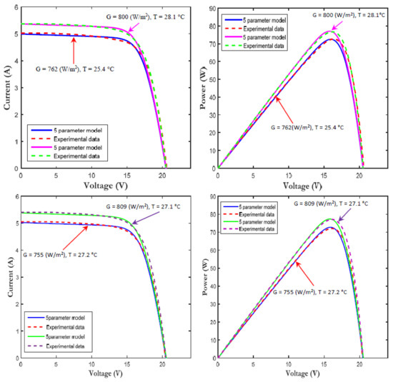
Figure 12.
Comparison between the experimental data and five-parameter model at various operating conditions.
Table 4.
RMS Errors calculated at various operating conditions.
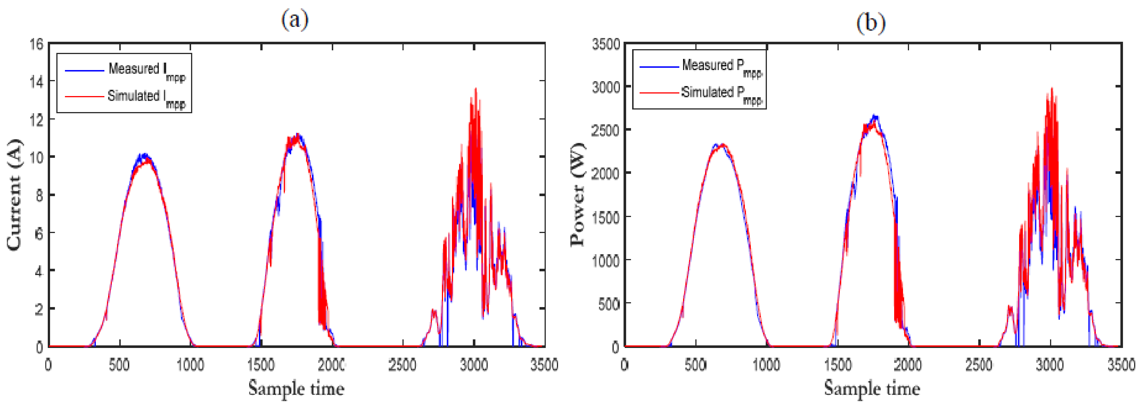
Once the five parameters at reference conditions are obtained, the resulting PV model can be used to predict time evolution of current at the maximum power point, voltage and power coordinates for the actual PV array. In Figure 13 it is shown the time evolution of both irradiance and temperature for three typical days (clear sky, semi-cloudy sky and cloudy sky). The corresponding measured and estimated current and power are reported in Figure 14.
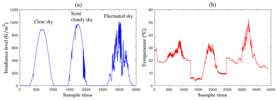
Figure 13.
Monitored irradiance (a) and Temperature (b) for three typical days (clear sky, semi-cloudy sky and cloudy sky).
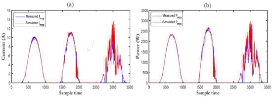
Figure 14.
(a) Measured vs estimated current at MPP, (b) measured vs estimated maximum power.
The obtained results are very close to the measured data, this can be further proved by calculating the exact difference between the measurements and simulated data by error indicators RMSE, MAPE and R2, as revealed by statistic metrics given in Table 5.
Table 5.
RMSE, R2, and MAPE for dynamic evolution of current and maximum power.
The main error metrics are given by the following expressions:
where xmpp,meas is the measured value, xmpp,sim is the correct simulated and N is the number of samples and the mean of the xmpp,meas is expressed as:
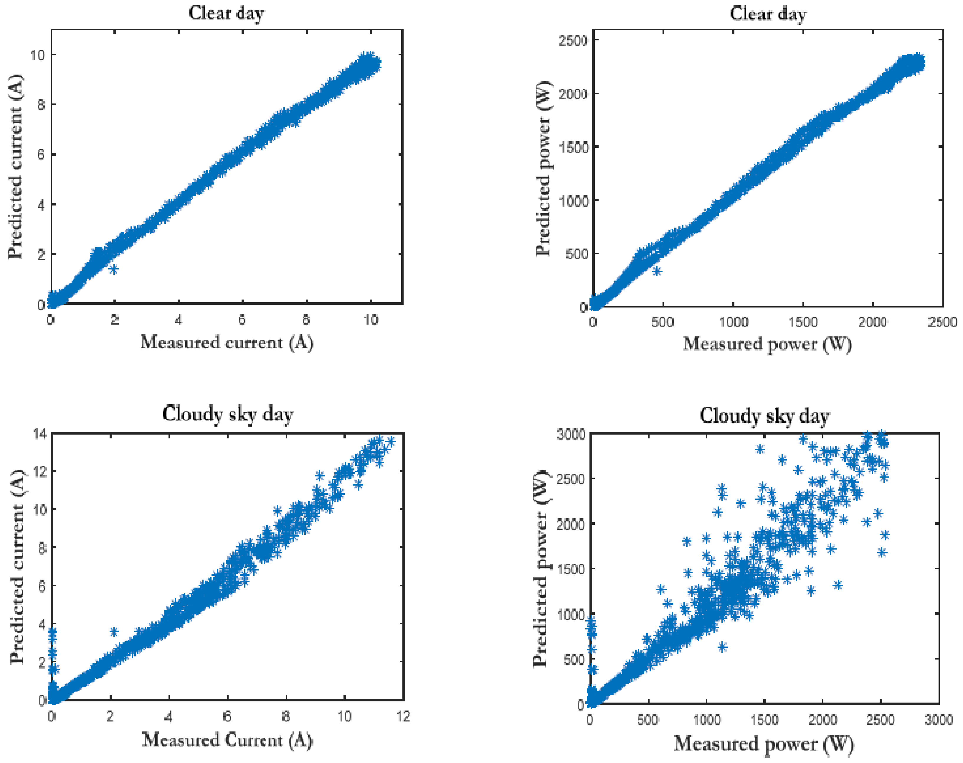
Table 6 reports the different error indicators for different daily irradiance and temperature. The results demonstrate the lowest values of these error indicators by observing the percentage of RMSE and MAPE errors obtained when using the extracted parameters from the proposed approach in the five-parameter model of the PV module. It can be seen that the obtained model reproduces the actual PV plant in a clear sky day as well as under changing climatic conditions. In Figure 15, the predicted and measured DC current and DC power are reported with good agreement between them.
Table 6.
Comparison between the measured and simulated power, current for different operating conditions.
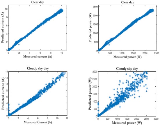
Figure 15.
Predicted and measured DC current and DC power for clear and cloudy sky day.
3.4. Comparison Study
In this section, a comparison study of the prediction model obtained by the manufacturer data, the proposed method and with those obtained by Newton-Raphson method.
In general, the manufacturer data do not provide satisfactory prediction results as the five parameters are given at standard test conditions. Particularly under changing environmental conditions, they cause noticeable deviation in the I-V curve especially in three key points, namely maximum power point (MPP), the ISC and at VOC point. Table 7 gives the comparison of the PV model parameters obtained by the proposed approach with those given by the manufacturer as well as those given by the Newton-Raphson method [40].
Table 7.
Comparison of the extracted parameters by different methods.
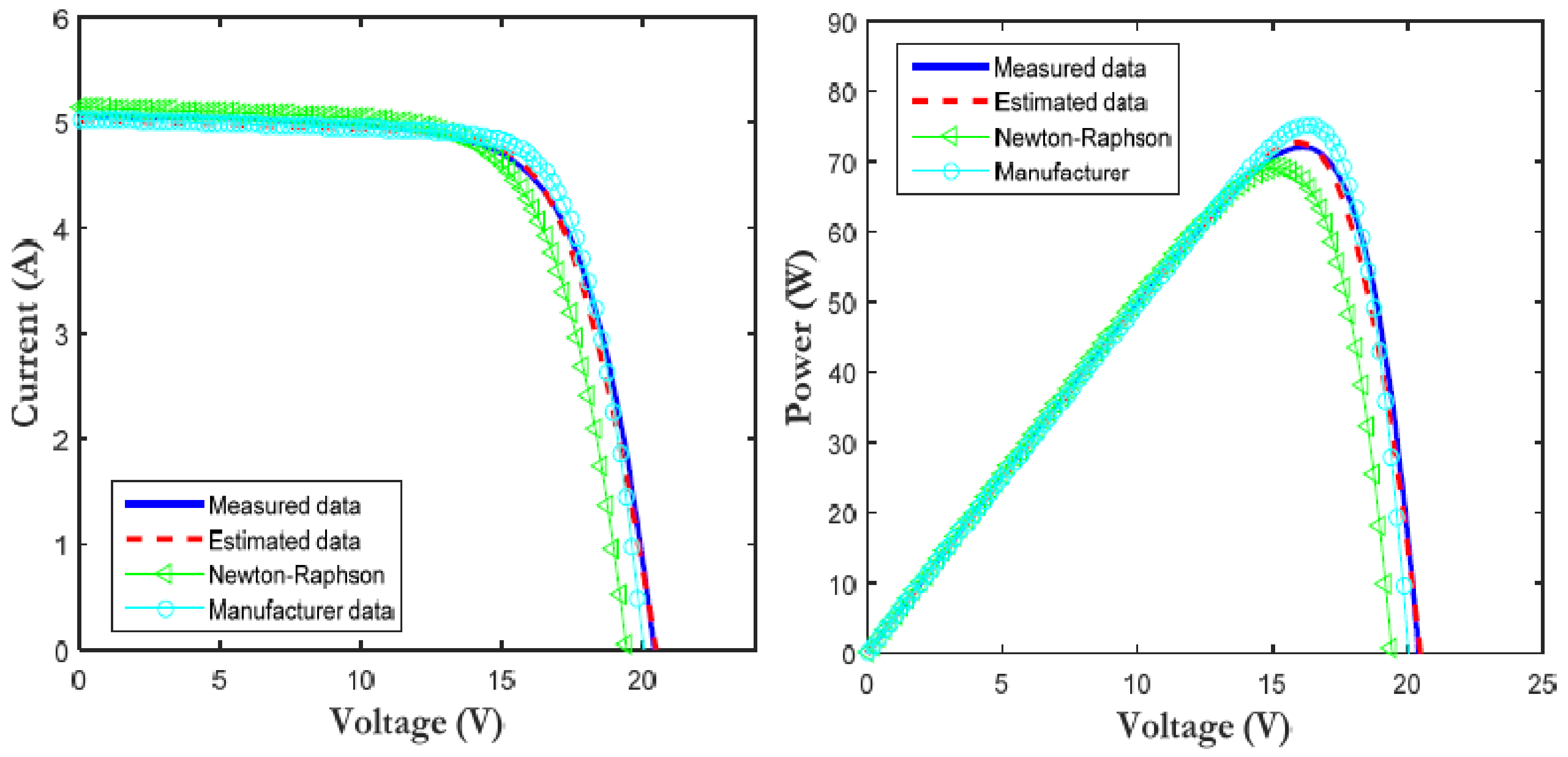
Figure 16 shows the different I-V and P-V curves obtained using the parameters given by the previously mentioned methods. The simulation is carried out under (G = 755 W/m2, T = 27.2 °C). By analyzing the curves, it seems that the results obtained by Newton-Raphson method, as well as the results obtained by parameters provided by the manufacturer, deviate significantly from the experimental curves, in particular at the maximum power point MPP, ISC and VOC. On the other hand, the I-V curves obtained by the proposed approach match the experimental curves in a way that makes them more precise than other methods. Additionally, to analyze the accuracy of the model, the root mean square (RMS) percentage is calculated for each method using Equation (19) (see Table 8).
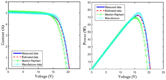
Figure 16.
Comparison between measured data, estimated, Newton-Raphson, manufacturer data: Current-Voltage and Power-Voltage curves at “G = 755 W/m2, T = 27.2 °C”.
Table 8.
RMS errors four five-parameter model.
4. Conclusions
In this paper, an improved and accurate approach to extract the five parameters of the single diode model of a PV module from the measured (I-V) curves is proposed. In this methodology, a hybrid approach was adopted where both analytical and numerical methods have been combined so that the extraction is achieved in three stages. First, the measured I-V characteristics under random conditions of irradiance and temperature are translated into standard test conditions using analytical formulas. In other words, the translation process provides a unique I-V curve at reference conditions. Then, with MFO algorithm as an optimization algorithm, the five parameters at reference conditions are extracted. These reference parameters are then used in the analytical expressions that describe PV modules at any working conditions. Unlike the developed methods in the literature, where the link of the five parameters with temperature and irradiance is not considered, the proposed methodology finds out the reference parameters using a metaheuristic optimization algorithm and then uses analytical formulations in which the irradiance and temperature are taken into account to find out the five parameters under random conditions. The estimated results obtained by the proposed approach were tested against measured static data (I-V curves) and measured dynamic data (time evolution of Impp, Vmpp and Pmpp). The results confirm the accuracy of this hybrid approach to estimate properly the five parameters and allow one to obtain an accurate model which can be used for energy prediction and fault diagnosis purposes.
Author Contributions
Conceptualization, S.A.H. and A.C.; formal analysis, A.C.; investigation, S.A.H. and A.C.; methodology, A.C. and S.M.; project administration, M.M.R. and A.M.K.; resources, S.M. and A.C.; supervision, A.C.; validation, A.C. and S.M.; visualization, S.M.; writing—original draft preparation, S.A.H.; writing—review and editing, A.C. All authors have read and agreed to the published version of the manuscript.
Funding
This research received no external funding.
Data Availability Statement
Data available on request due to restrictions eg privacy or ethical.
Acknowledgments
This work was supported in part by the “Direction Generale de la Recherche Scientifique et du Développement Technologique, DGRSDT” of Algeria.
Conflicts of Interest
The authors declare no conflict of interest.
References
- Chaibi, Y.; Allouhi, A.; Salhi, M. A simple iterative method to determine the electrical parameters of photovoltaic cell. J. Clean. Prod. 2020, 269, 122363. [Google Scholar] [CrossRef]
- Mao, M.; Zhang, L.; Huang, H.; Chong, B.; Zhou, L. Maximum power exploitation for grid-connected PV system under fast-varying solar irradiation levels with modified salp swarm algorithm. J. Clean. Prod. 2020, 268, 122158. [Google Scholar] [CrossRef]
- Chouder, A.; Silvestre, S. Automatic supervision and fault detection of PV systems based on power losses analysis. Energy Convers. Manag. 2010, 51, 1929–1937. [Google Scholar] [CrossRef]
- Dhimish, M.; Holmes, V.; Mehrdadi, B.; Dales, M. Comparing Mamdani Sugeno fuzzy logic and RBF ANN network for PV fault detection. Renew. Energy 2018, 117, 257–274. [Google Scholar] [CrossRef] [Green Version]
- Kichou, S.; Silvestre, S.; Nofuentes, G.; Torres-Ramírez, M.; Chouder, A.; Guasch, D. Characterization of degradation and evaluation of model parameters of amorphous silicon photovoltaic modules under outdoor long term exposure. Energy 2016, 96, 231–241. [Google Scholar] [CrossRef]
- Dash, V.; Bajpai, P. Power management control strategy for a stand-alone solar photovoltaic-fuel cell-battery hybrid system. Sustain. Energy Technol. Assess. 2015, 9, 68–80. [Google Scholar] [CrossRef]
- Mahmoud, Y.A.; Xiao, W.; Zeineldin, H.H. A Parameterization Approach for Enhancing PV Model Accuracy. IEEE Trans. Ind. Electron. 2012, 60, 5708–5716. [Google Scholar] [CrossRef]
- Triki-Lahiani, A.; Bennani-Ben Abdelghani, A.; Slama-Belkhodja, I. Fault detection and monitoring systems for photovoltaic installations: A review. Renew. Sustain. Energy Rev. 2018, 82, 2680–2692. [Google Scholar] [CrossRef]
- Moshksar, E.; Ghanbari, T. Adaptive Estimation Approach for Parameter Identification of Photovoltaic Modules. IEEE J. Photovolt. 2017, 7, 614–623. [Google Scholar] [CrossRef]
- De Soto, W.; Klein, S.A.; Beckman, W.A. Improvement and validation of a model for photovoltaic array performance. Sol. Energy 2006, 80, 78–88. [Google Scholar] [CrossRef]
- Villalva, M.G.; Gazoli, J.R.; Filho, E.R. Comprehensive Approach to Modeling and Simulation of Photovoltaic Arrays. IEEE Trans. Power Electron. 2009, 24, 1198–1208. [Google Scholar] [CrossRef]
- Siddique, H.A.B.; Xu, P.; De Doncker, R.W. Parameter extraction algorithm for one-diode model of PV panels based on datasheet values. In Proceedings of the 2013 International Conference on Clean Electrical Power (ICCEP), Alghero, Italy, 11–13 June 2013; pp. 7–13. [Google Scholar] [CrossRef]
- Lo Brano, V.; Orioli, A.; Ciulla, G.; Di Gangi, A. An improved five-parameter model for photovoltaic modules. Sol. Energy Mater. Sol. Cells 2010, 94, 1358–1370. [Google Scholar] [CrossRef]
- Carrero, C.; Ramírez, D.; Rodríguez, J.; Platero, C.A. Accurate and fast convergence method for parameter estimation of PV generators based on three main points of the I–V curve. Renew. Energy 2011, 36, 2972–2977. [Google Scholar] [CrossRef]
- Zagrouba, M.; Sellami, A.; Bouaïcha, M.; Ksouri, M. Identification of PV solar cells and modules parameters using the genetic algorithms: Application to maximum power extraction. Sol. Energy 2010, 84, 860–866. [Google Scholar] [CrossRef]
- Low, K.S.; Soon, J.J. Photovoltaic model identification using particle swarm optimization with inverse barrier constraint. IEEE Trans. Power Electron. 2012, 27, 3975–3983. [Google Scholar]
- Jiang, L.L.; Maskell, D.L.; Patra, J.C. Parameter estimation of solar cells and modules using an improved adaptive differential evolution algorithm. Appl. Energy 2013, 112, 185–193. [Google Scholar] [CrossRef]
- Askarzadeh, A.; Rezazadeh, A. Artificial bee swarm optimization algorithm for parameters identification of solar cell models. Appl. Energy 2013, 102, 943–949. [Google Scholar] [CrossRef]
- Oliva, D.; Cuevas, E.; Pajares, G. Parameter identification of solar cells using artificial bee colony optimization. Energy 2014, 72, 93–102. [Google Scholar] [CrossRef]
- Patel, S.J.; Panchal, A.K.; Kheraj, V. Extraction of solar cell parameters from a single current-voltage characteristic using teaching learning based optimization algorithm. Appl. Energy 2014, 119, 384–393. [Google Scholar] [CrossRef]
- Askarzadeh, A.; Dos Santos Coelho, L. Determination of photovoltaic modules parameters at different operating conditions using a novel bird mating optimizer approach. Energy Convers. Manag. 2015, 89, 608–614. [Google Scholar] [CrossRef]
- Alam, D.F.; Yousri, D.A.; Eteiba, M.B. Flower Pollination Algorithm based solar PV parameter estimation. Energy Convers. Manag. 2015, 101, 410–422. [Google Scholar] [CrossRef]
- Kang, T.; Yao, J.; Jin, M.; Yang, S.; Duong, T. A novel improved cuckoo search algorithm for parameter estimation of photovoltaic (PV) models. Energies 2018, 11, 1060. [Google Scholar] [CrossRef] [Green Version]
- Chen, X.; Yu, K.; Du, W.; Zhao, W.; Liu, G. Parameters identification of solar cell models using generalized oppositional teaching learning based optimization. Energy 2016, 99, 170–180. [Google Scholar] [CrossRef]
- Ben Messaoud, R. Extraction of uncertain parameters of double-diode model of a photovoltaic panel using Ant Lion Optimization. SN Appl. Sci. 2020, 2, 239. [Google Scholar] [CrossRef] [Green Version]
- Tatabhatla, V.M.R.; Agarwal, A.; Kanumuri, T. Performance enhancement by shade dispersion of Solar Photo-Voltaic array under continuous dynamic partial shading conditions. J. Clean. Prod. 2018, 213, 462–479. [Google Scholar] [CrossRef]
- Han, W.; Wang, H.; Chen, L. Parameters Identification for Photovoltaic Module Based on an Improved Artificial Fish Swarm Algorithm. Sci. World J. 2014, 2014, 12. [Google Scholar] [CrossRef] [PubMed] [Green Version]
- Jack, V.; Salam, Z.; Ishaque, K. Cell modelling and model parameters estimation techniques for photovoltaic simulator application: A review. Appl. Energy 2015, 154, 500–519. [Google Scholar] [CrossRef]
- Chine, W.; Mellit, A.; Lughi, V.; Malek, A.; Sulligoi, G.; Pavan, A.M. A novel fault diagnosis technique for photovoltaic systems based on artificial neural networks. Renew. Energy 2016, 90, 501–512. [Google Scholar] [CrossRef]
- Hadj Arab, A.; Chenlo, F.; Benghanem, M. Loss-of-load probability of photovoltaic water pumping systems. Sol. Energy 2004, 76, 713–723. [Google Scholar] [CrossRef]
- Mirjalili, S. Moth-flame optimization algorithm: A novel nature-inspired heuristic paradigm. Knowl.-Based Syst. 2015, 89, 228–249. [Google Scholar] [CrossRef]
- Garoudja, E.; Kara, K.; Chouder, A.; Silvestre, S. Parameters extraction of photovoltaic module for long-term prediction using artifical bee colony optimization. In Proceedings of the 2015 3rd International Conference on Control, Engineering & Information Technology (CEIT), Tlemcen, Algeria, 25–27 May 2015. [Google Scholar] [CrossRef]
- Chouder, A.; Silvestre, S.; Sadaoui, N.; Rahmani, L. Modeling and simulation of a grid connected PV system based on the evaluation of main PV module parameters. Simul. Model. Pract. Theory 2012, 20, 46–58. [Google Scholar] [CrossRef]
- Elkholy, A.; El-Ela, A.A. Optimal parameters estimation and modelling of photovoltaic modules using analytical method. Heliyon 2019, 5, e02137. [Google Scholar] [CrossRef] [PubMed]
- Tossa, A.K.; Soro, Y.M.; Azoumah, Y.; Yamegueu, D. A new approach to estimate the performance and energy productivity of photovoltaic modules in real operating conditions. Sol. Energy 2014, 110, 543–560. [Google Scholar] [CrossRef]
- Karaboga, D. An Idea Based on Honey Bee Swarm for Numerical Optimization. 2005. Available online: https://abc.erciyes.edu.tr/pub/tr06_2005.pdf (accessed on 1 January 2005).
- Kennedy, J.; Eberhart, R. Particle Swarm Optimisation. In Proceedings of the ICNN’95—International Conference on Neural Networks, Perth, Australia, 27 November–1 December 1995; pp. 1942–1948. [Google Scholar] [CrossRef]
- Rainer, S.; Kenneth, P. Differential Evolution: A Simple and Efficient Heuristic for Global Optimization over Continuous Spaces. J. Glob. Optim. 1997, 11, 341. [Google Scholar]
- Rao, R.V.; Savsani, V.J.; Vakharia, D.P. Teaching-Learning-Based Optimization: An optimization method for continuous non-linear large scale problems. Inf. Sci. 2012, 183, 1–15. [Google Scholar] [CrossRef]
- Yetayew, T.T.; Jyothsna, T.R. Parameter extraction of photovoltaic modules using Newton Raphson and simulated annealing techniques. In Proceedings of the 2015 IEEE Power, Communication and Information Technology Conference (PCITC), Bhubaneswar, India, 15–17 October 2016; pp. 229–234. [Google Scholar] [CrossRef]

Publisher’s Note: MDPI stays neutral with regard to jurisdictional claims in published maps and institutional affiliations. |
© 2021 by the authors. Licensee MDPI, Basel, Switzerland. This article is an open access article distributed under the terms and conditions of the Creative Commons Attribution (CC BY) license (https://creativecommons.org/licenses/by/4.0/).