Analysis of Complex Solid-Gas Flow under the Influence of Gravity through Inclined Channel and Comparison with Real-Time Dual-Sensor System

Abstract

Gas-solid flow is used in the chemical industry, food industry, pharmaceuticals, vehicles, and power generation. The calculation of flow has aroused great interest in contemporary industry. In recent decades, researchers have been seeking to build an effective system to monitor and calculate gas-solid flow. Attempts have been extended from computational modeling to the creation of flow pattern visualization methods and mass flow (MFR) quantification. MFR is usually studied by volume flow concentration (VFC) and velocity distribution of solid particles. A non-invasive device is used for testing MFR, in which electronic and mechanical sensors are used to balance the shortcomings related to each other. This study investigates the simulation of flow patterns to demonstrate the behavior of solid particles as they pass through the channel. The particles are allowed to slide longitudinally in the insulated tending channel. This slippage is due to the influence of natural gravity. Electronic sensor components are used to measure the velocity distribution and concentration of volumetric flow. The load cell is used as an auxiliary sensor for measuring MFR. In addition, ANSYS fluent is used to analyze streaming queries. The experimental results are related to evaluating the accuracy and relative error of the data collected from various sensors under different conditions. However, the simulation results can help explain the movement of the gas-solid mixture and can understand the cause of pipeline blockage during the slow movement of solid particles.

1. Introduction

The latest transformation in industry has driven scientists and engineers to implement new instrumentation methods in real-time tracking and computing of two-phase flow, such as solid-gas [1]. Ever tightening resources and arbitrary working environments of process plants would promote adequate instrumentation for solid particle transportation. The expression ‘gas-solid flow’ is a rate at which solid matter flows through a channel per unit time. An effective MFR calculates particles moving through the pipe by quantifying the system’s velocity profile and volumetric flow concentration. Since classical mechanics in conjunction with computer science produced an innovative environment for computational fluid dynamics (CFD), the partial differential equations for fluids that were tough to handle converted to simple algebraic equations for flow dynamics that quickly conclude the numerical solution for the situation under study [2]. The CFD works by dividing computational domains of the problem into smaller domains, setting boundary conditions for boundary nodes, and instigating estimates to generate a linear algebraic equation system that can compute the pressure, temperature, and velocity fields in the desired region. The CFD is also applied on solid particles and fluids to determine said parameters in a region [3].

Several sensing methods have been studied, including flow detectors, flow meters, and velocity and pressure sensors. However, there is already a problem with using these measurement-based sensing methods. The capacitive and electrostatic sensing techniques are more desirable and promising than other sensing techniques. There are distinct characteristics of low manufacturing cost that make them an appealing alternative to conventional approaches. These methods are non-invasive, rapid response, contact-free, non-disruptive, maintenance-free, radiation-free, and highly precise for flow measurement [4]. Capacitive sensing methods frame on electrodes. These electrodes possess single or several pairs that gain an electrical signal when an external voltage is applied. If the medium in its proximity is changed, the electric field affects the charges (dielectric constant). The amount of change the sensor creates is determined and provides knowledge about its environment. The details, including change of the particle velocity, particle flow concentration, and particle MFR, are interpreted based on the difference in capacitance values. Gas-solid flow calculations operate based on differing electrical properties of the mixture, flowing via the sensing volume [5]. Various researchers have participated in the study of capacitive sensing. These methods research the powder flow principle in the manufacturing world [6]. The VFC can calculate from the capacitance between the sensing electrodes and passage of the material via the channel in between the electrodes [7,8]. Hu et al. [9] developed a capacitive-type sensor. This sensor tests the concentration of pulverized coal for laboratory use. A stainless-steel source grid deploys to increase the sensitivity of the capacitance sensors to counteract the disadvantageous effect of the environment. However, there are drawbacks of methods for treating non-homogeneous stable particles.

Ismail et al. [10] and Holler et al. [11] focused on the advancement of capacitive sensing technologies and applying them to manufacturing. However, their capacitance sensor does not work properly at higher resolutions. Brasseur et al. [12] studied the impact of dampness and dewdrops that remain intact with sensors and induce contamination that is conductive in nature and did not correlate to findings of mechanical assembly. Bretterklieber et al. [13] explained a separate capacitance to digital conversion approach by employing IC circuits; nonetheless, analogue to digital conversion causes a delay in online tracking. Sun et al. [14] studied a pneumatic accumulation of pulverized coal in a two-phase gas-solid flow. This design uses source-grid sensing electrodes by interrelated double sample and a lock-in detector for higher and unvarying capacitance sensing in the pipe cross-section. The outcome of the flow regime in the calculation of concentration (less than 5% in the simulated environment) [14] is thus minimized. Despite this strategy, it has problems with longer run simulations.

In the early work of [15], we worked on designing real-time dual-sensors for MFR. However, this work does not cover the complicated gas-solid two-state particle flow. In addition, it does not cover comparative analysis with simulation results and real-time values. The data fusion of electrical and mechanical sensors is also not discussed.

We have summarized the key contributions of this paper as follows:

• The gas-solid flow, non-invasive, real-time measurement and monitoring are studied in this paper, including the mass flow rate (MFR) of solid particles.
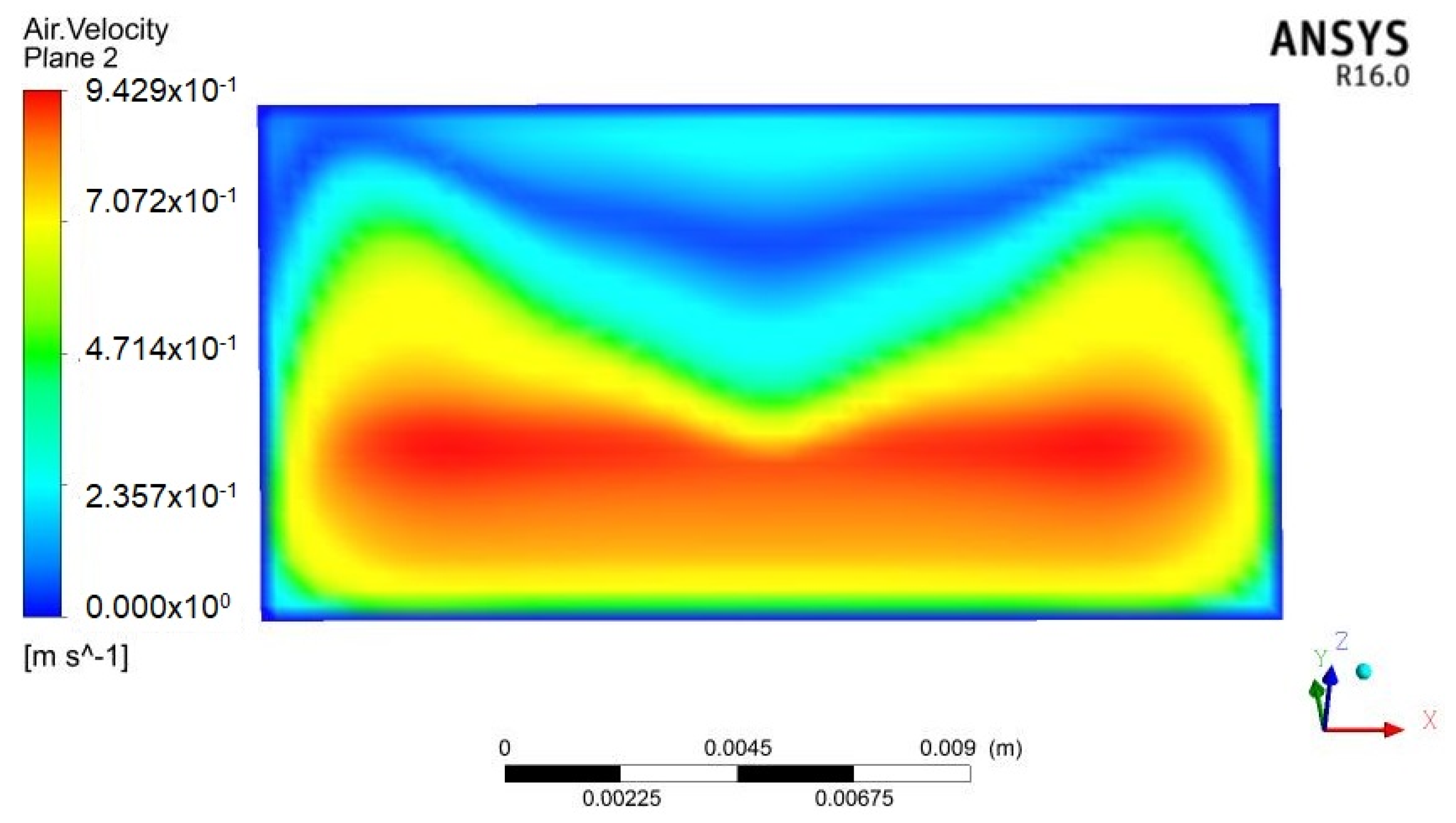
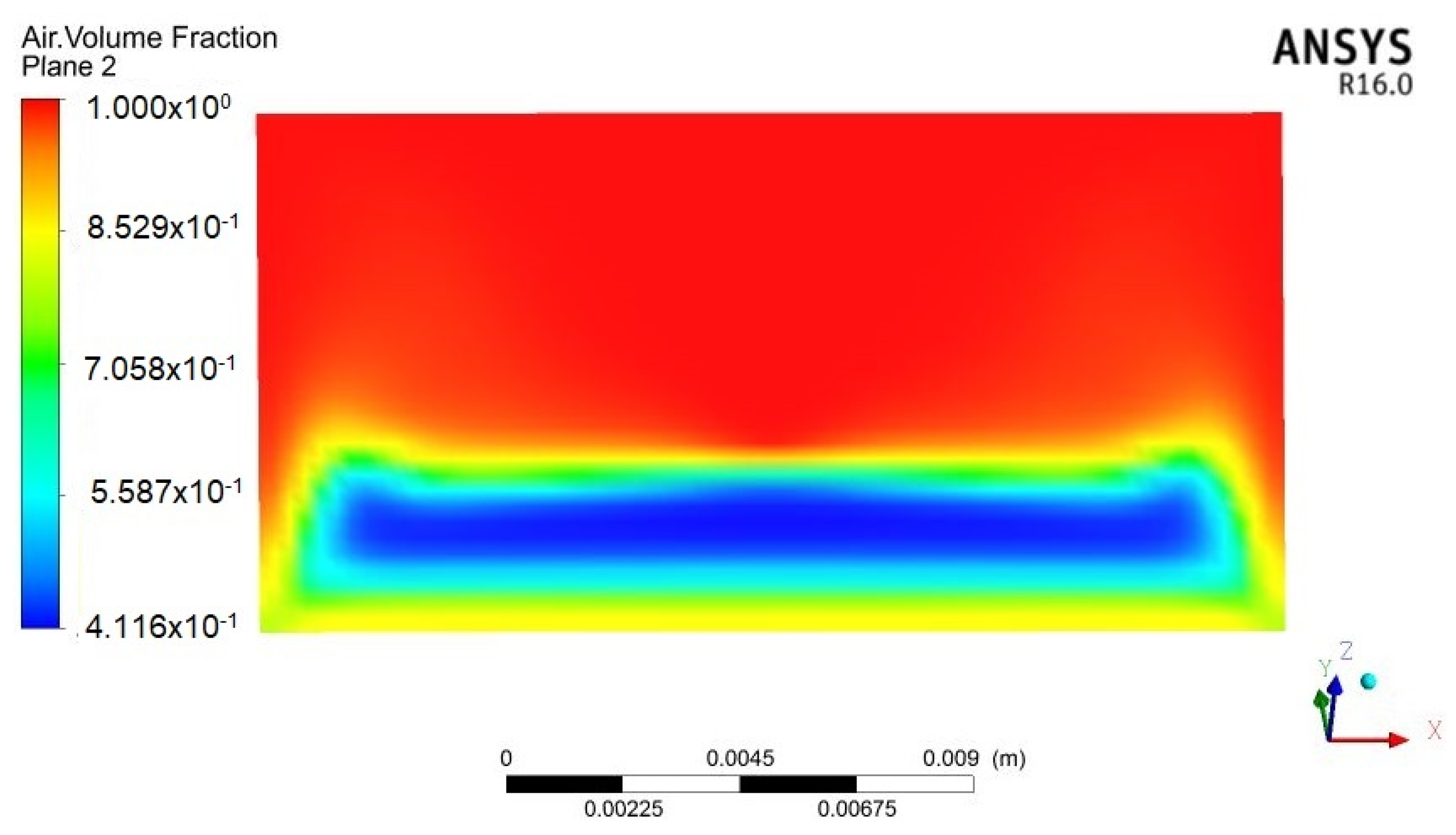
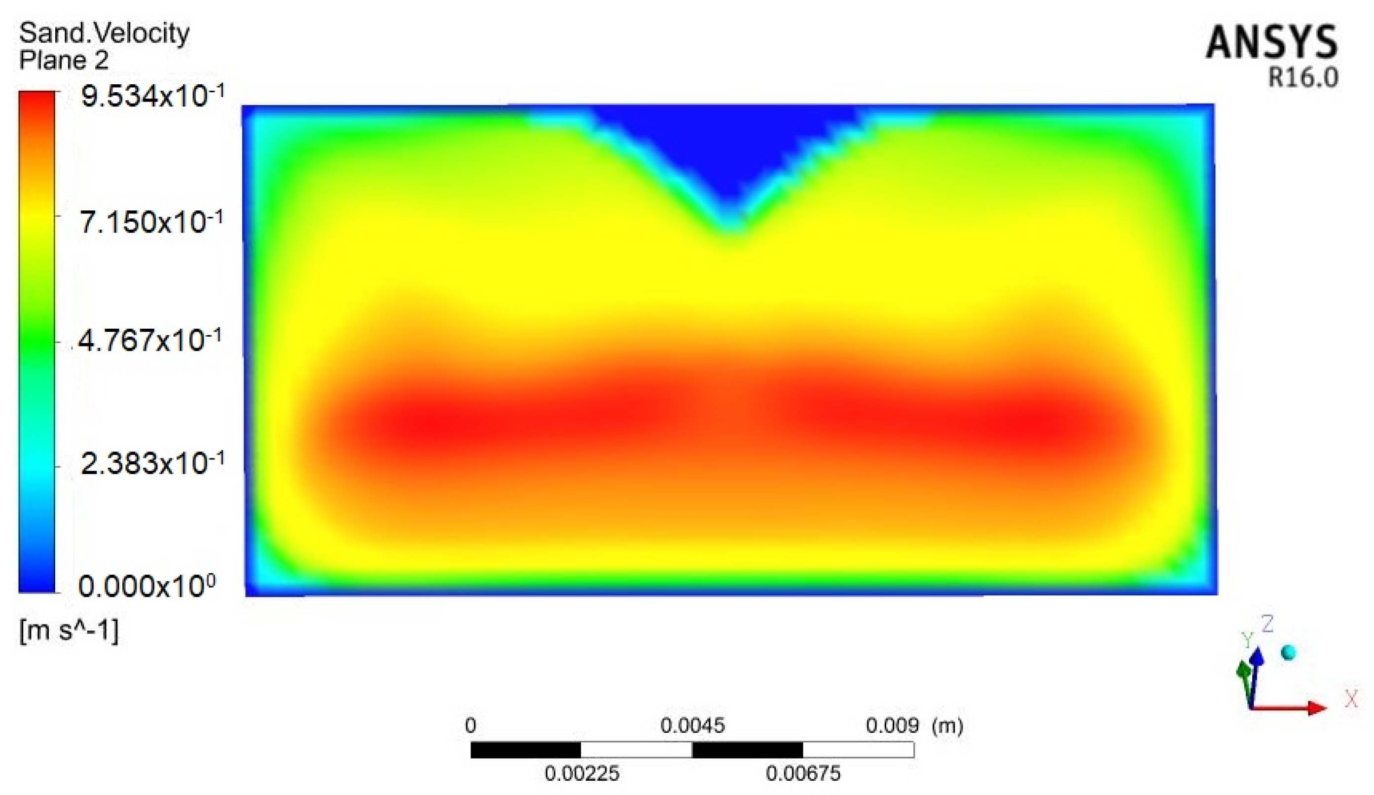
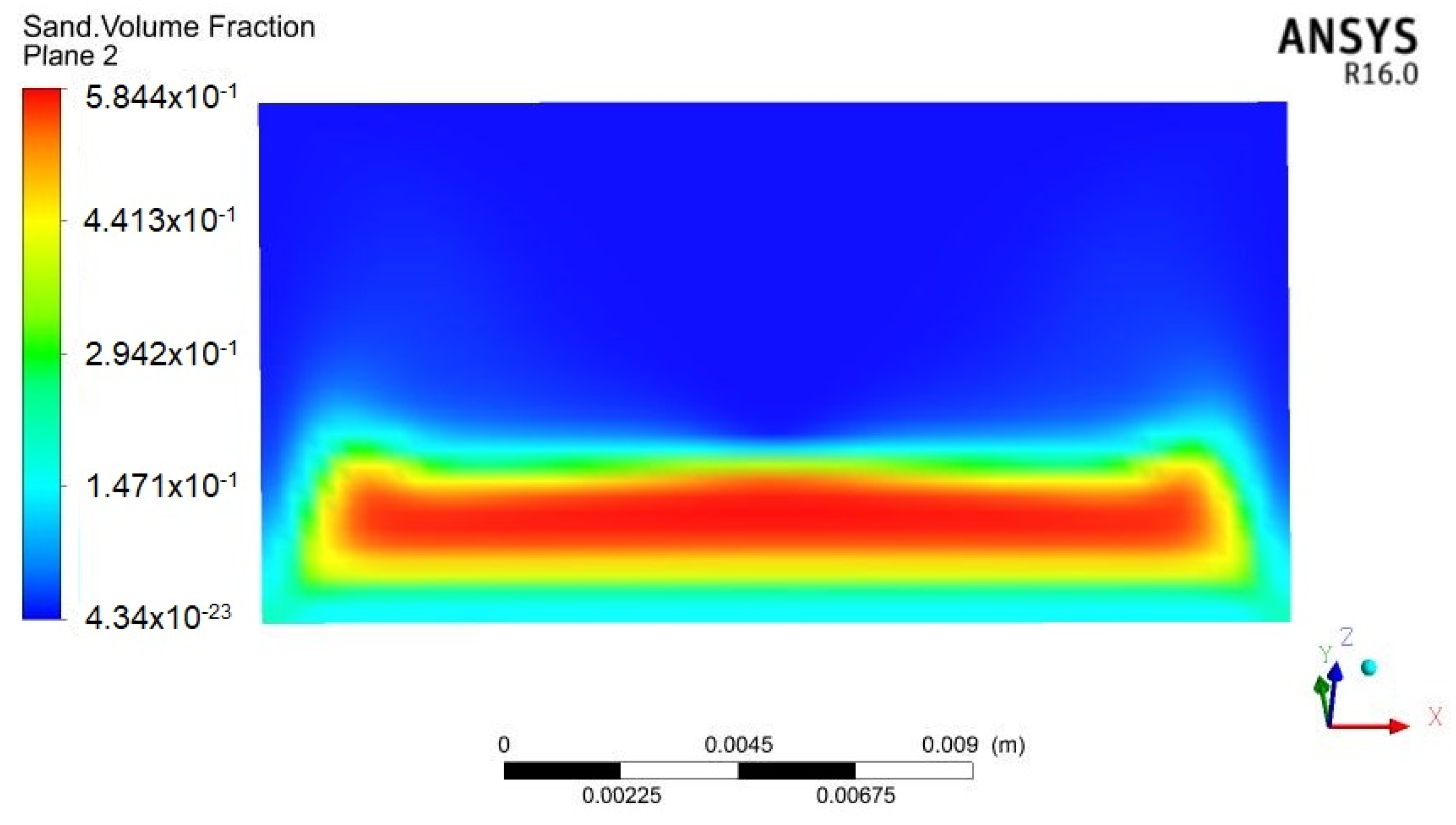
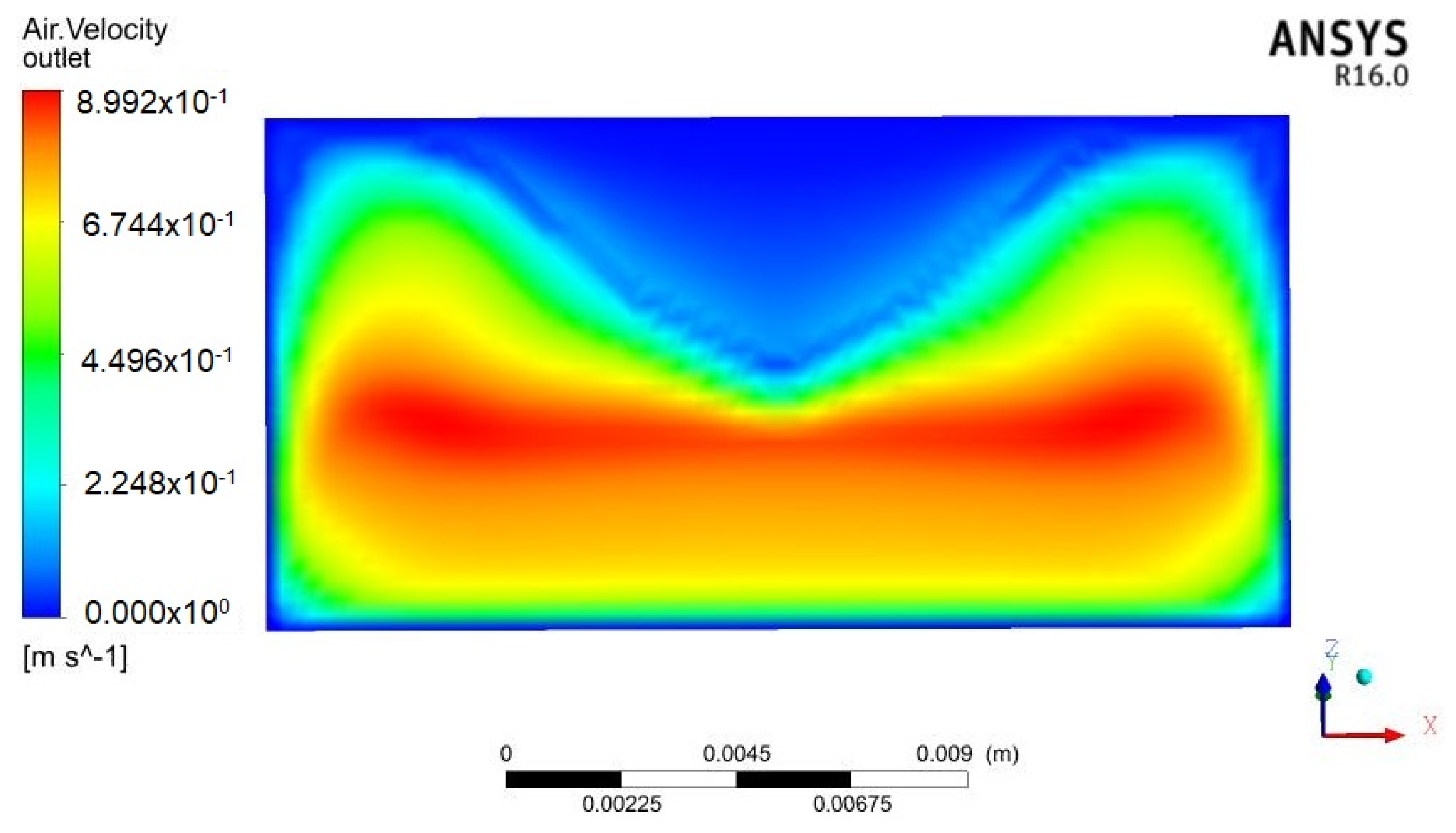
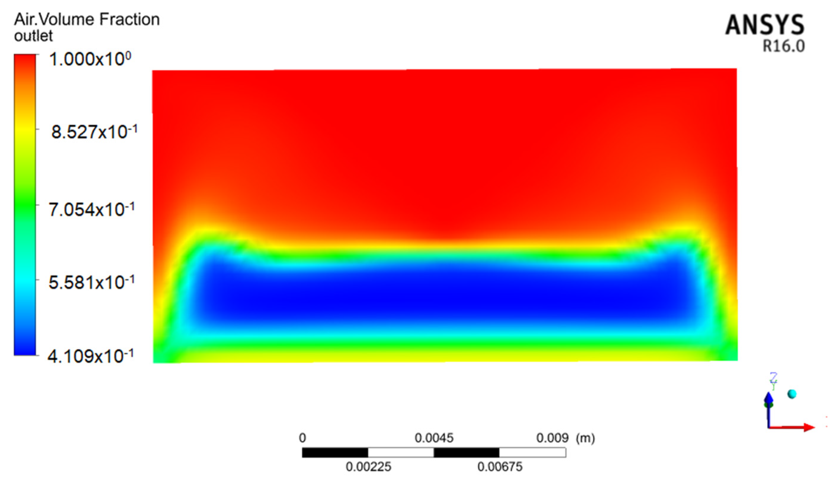
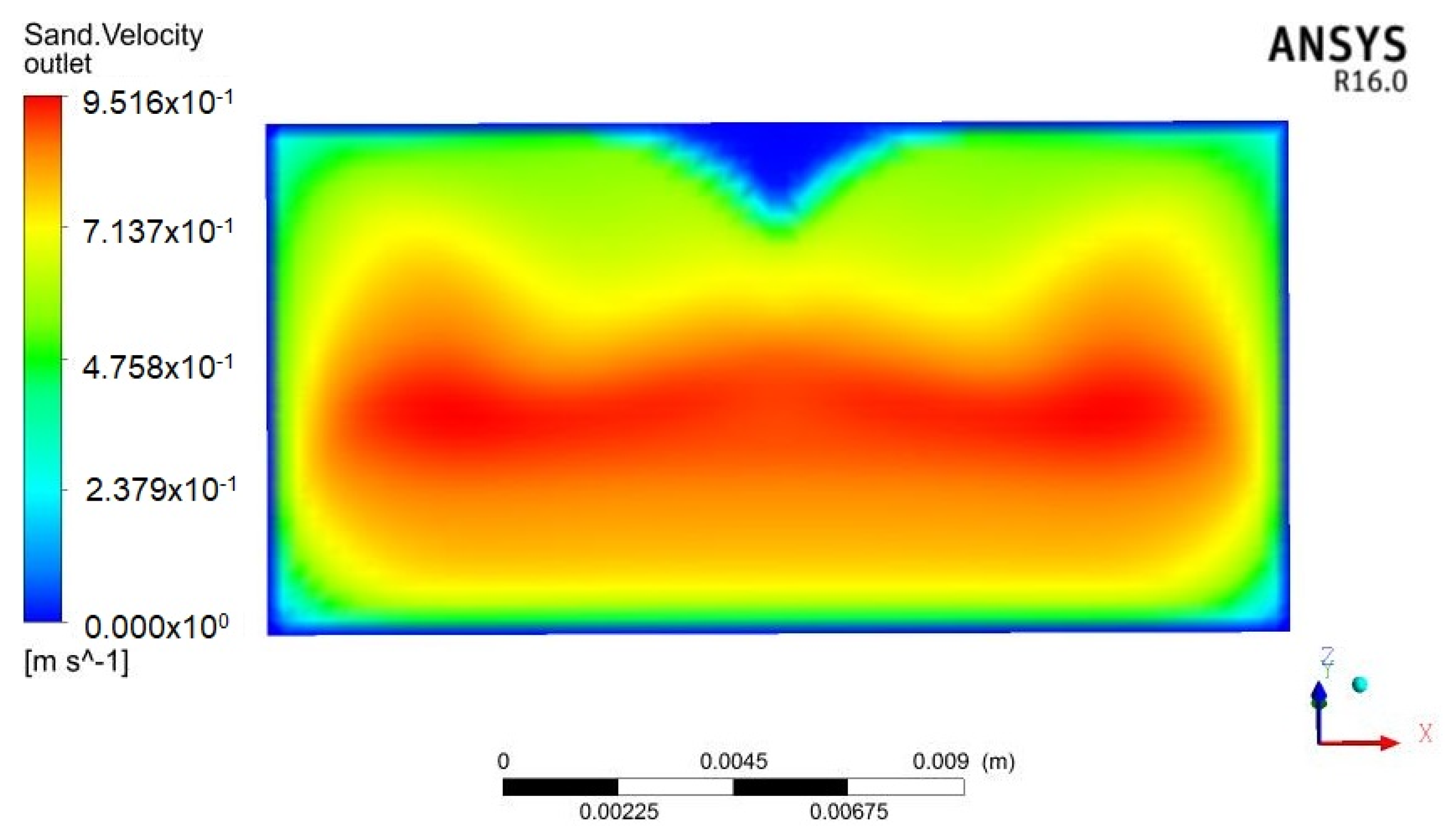
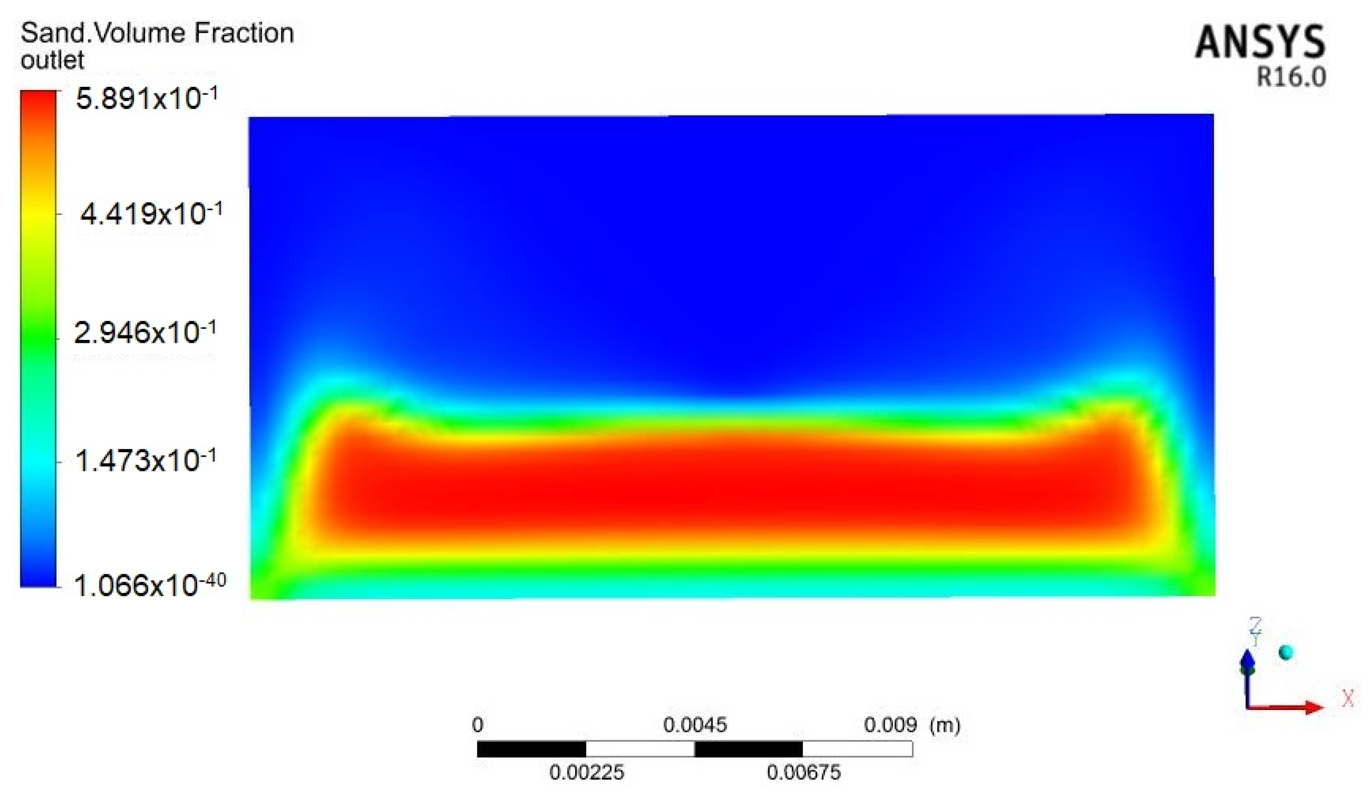
• Due to the bonding of solid particles, there is a serious problem of gas-solid flow pipe and conduit blockage in a large number of processing industries. In response to this problem, the paper uses specialized simulation tools (ANSYS R16.0 FLUENT) to study the effects of gravity on the flow of solid-state particles in the inclined channel [4] and to focus on the behavior of pneumatic sand flow in the tilt channel to provide insight into the problem of the gas-solid flow pipe and conduit blockage.
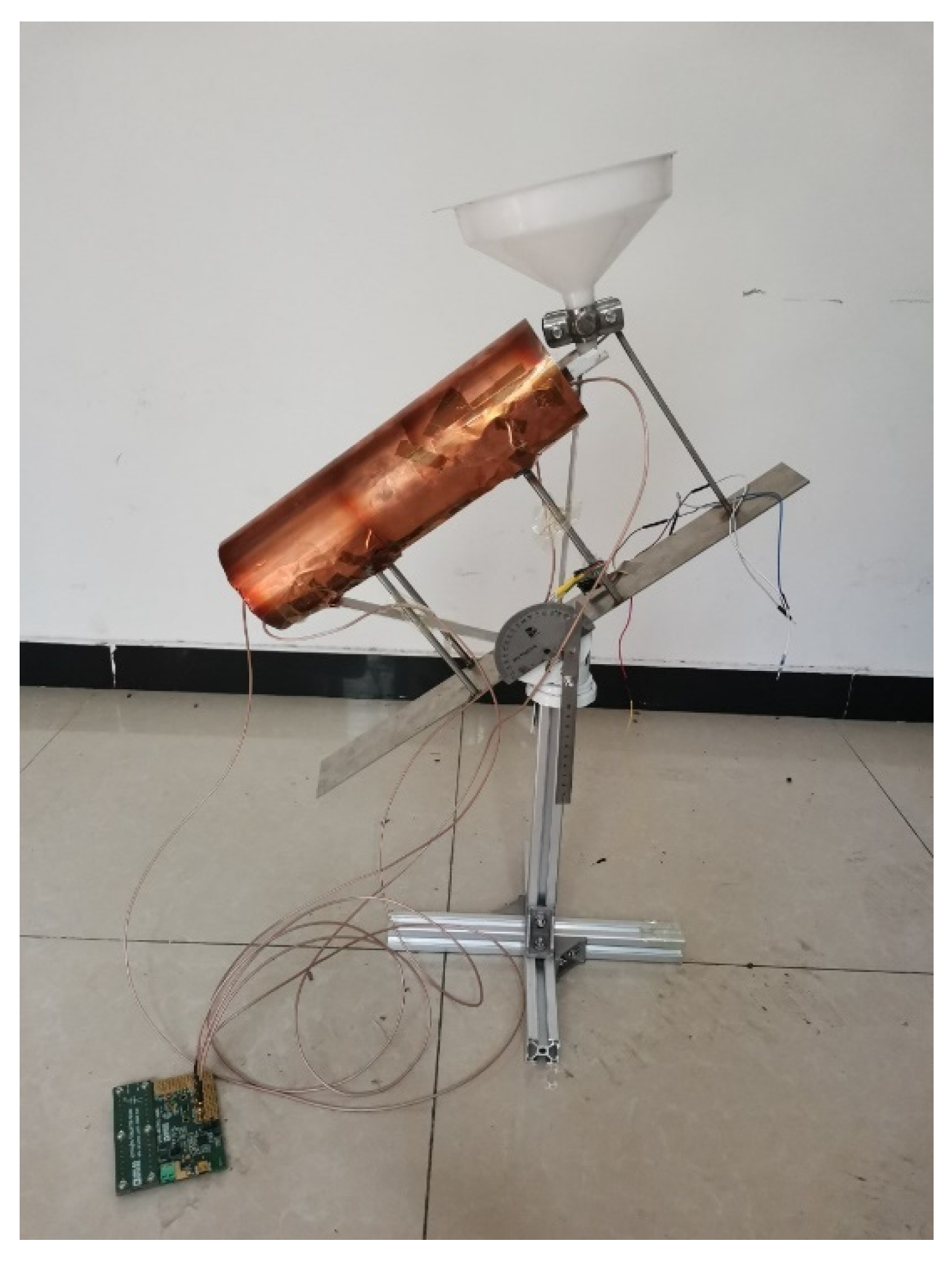
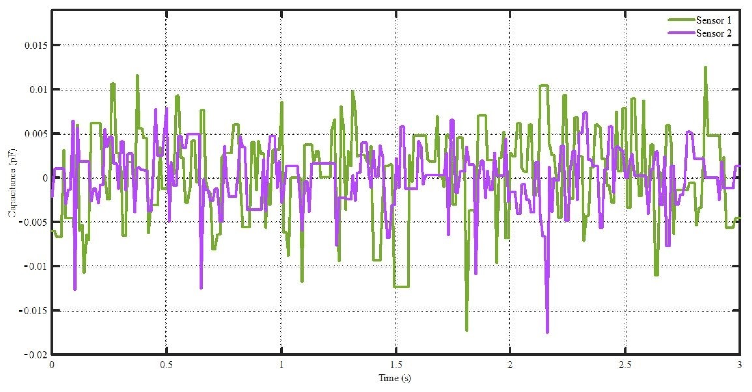
• This paper employed a dual-sensor approach (electrical and mechanical sensors) for invasive solid MFR measurement to complete a new measurement and monitoring system design using the advantages of both the sensors. Among these, the flow rate profile and volume flow concentration of solid particles are calculated based on the data collected by electrical sensors, while the MFR of solid particles is the responsibility of the mechanical load sensor.
• Data fusion was applied to the results of both sensors to enhance the accuracy closer to the true values. This arrangement consists of a load cell connected at the lower side of the tube and two capacitive electrodes situated along the channel’s walls.
• Our proposed sensor architecture compares well to alternatives and is appropriate for the proposed application in the research field.

The rest of this paper is organized as follows. Section 2 defines the measurement principle, whereas data fusion of the sensor to the actual value and solid flow simulations are explained in Section 3 and Section 4, respectively. Section 5 describes the measurement system used. Section 6 presents the results and discussion, and the paper is concluded in Section 7.

2. Measurement Principles

This research focused on the fabrication of sensors. These designed sensors apply for calculating the MFR of solid particles. There are two kinds of techniques: (1) indirect and (2) direct methods of calculation [15]. These methods are explained in subsequent sections.

2.1. Indirect Measurement (by Electrical Sensor)

The MFR of solid particles through a cross-section of a channel is calculated by applying Equation (1) [16]:

$$M\left(t\right)={\rho }_{s}A{V}_s\left(t\right){\beta }_s\left(t\right)$$

(1)

where $M$ is the MFR of the solid particles, $A$ is an area in the cross-section of the channel through which the particles flow, the average concentration of volumetric flow is depicted by ${\beta }_s\left(t\right)$, whereas the mean velocity of particles is $V_s\left(t\right)$ and for the density of the following particles, ${\rho }_s$ is employed [14,15].

2.1.1. Measurement of Velocity

The airborne solid particles flow in between the capacitive region inside sensing electrodes. These particles display changes in dielectric properties. These changes produce capacitance differences among sensing electrodes. As a result of this phenomenon, many sensors are used to study particle movement, particularly the flow of gas and solids [17,18]. This electrical sensor is either a capacitive sensor, a resistor sensor, or an electrostatic sensor. This algorithm is known as cross-correlation. Abrar et al. [15] have illustrated phenomena of cross-correlation flow utilizing capacitive sensors.

The experimental setup for this research is shown in Figure 1. Two capacitive sensors are placed on a channel. The channel has a known axial spacing, i.e., D. The sensors are time-synchronized and excited using the same signal. At the time of particle flow from the top (i.e., first) to the lower (i.e., second) sensor, the sensors show variation in the values of capacitance. These variations are measured and recorded simultaneously. During this flow, both sensors display similar variation patterns. The only difference in patterns is a time delay. The cross-correlation of output signals between the two sensors is calculated by Equation (2) [18]. The time coordinate that provides the maximum value for $C\left[m\right]$ denotes transit time, ${\tau }_{max}$, for the moving solid particles. Equation (3) [17] is used to calculate the velocity of particles.

$$C\left[m\right]=\frac{1}{L}{\displaystyle \sum }_{n=0}^{L}a\left[n\right]\cdot b\left[n+m\right]$$

(2)

$$V=\frac{D}{{\tau }_{max}}$$

(3)

In a real-time situation, an interval of sampling is very significant. Slow or fast sampling will generate a time delay, hence varying precision in the transit time calculation [19]. The sampling interval preference is based upon the characteristics of the electrodes used, the type of channel, and its geometry. Naturally, rapid sampling results in a lower relative error for the transit time calculation; nevertheless, particle flow instability can result otherwise. The time required for sample integration is also crucial for cross-correlation calculation. Typically, transit time samples are selected as at least ten times the sampling interval [20]. As the integration time increases, the transit time calculation will become more precise. Therefore, calculating the velocity is sluggish, and collecting the data takes time.

2.1.2. Concentration of Volumetric Flow

The capacitance of the electrodes in the channel varies in the case of two-phase flow, i.e., gas-solid flow in this paper. These changes in capacitance values are used to infer volumetric flow concentration through appropriate calibration and mathematical modeling. In addition, electrode geometry and dielectric material permittivity affect the capacitance value, as represented in Equation (4) [11]:

$$C=C_{0}h\left({\epsilon }_r\right)$$

(4)

where $C_0$ is the value capacitance of electrodes at the time of no or zero flow, and typically the sensor’s shape determines its values. $h\left({\epsilon }_r\right)$ is proportional to particle concentration while using parallel capacitors. A higher flow concentration results in larger capacitance values amongst the electrodes, and vice versa [21]. However, certain anomalies may result in inaccuracies. One of the main causes of errors is the inhomogeneous distribution of sensitivity among the electrodes. A pair of parallel plate capacitors is used to cover both the upper and lower surfaces of the channel. All solid particle flowing is required to pass between the sensing gap of electrodes to avoid this measurement inaccuracy.

2.2. Direct Measurement (by Mechanical Sensor)

Typically, load cells are mounted on the blow/receiving tank to determine the MFR. This strategy is not suited to large-scale conveying systems since load cells constructed for greater weight values are less precise than those premeditated for lower weight values. In case a load cell is placed at the base of a trivial, specified channel segment, the device can calculate MFR more accurately [22]. A cross-sectional MFR is computed using Equation (5) [22], where $V$ is the cross-correlation velocity and $m$ is the value of the load cell attached at the base of the known length channel, $l$, observing a steady flow.

$$MFR=\frac{m}{l}\cdot V$$

(5)

A steady-state flow of solid particles travelling lengthwise along the lower surface of a channel as a discrete dense phase material by natural gravitation can be described by Equation (5). They dispersed in case particles under observation were pneumatically carried in the air [23]. This could cause mistakes in load cell measurements. However, the dilution of suspended solid particles does not influence capacitive measurements.

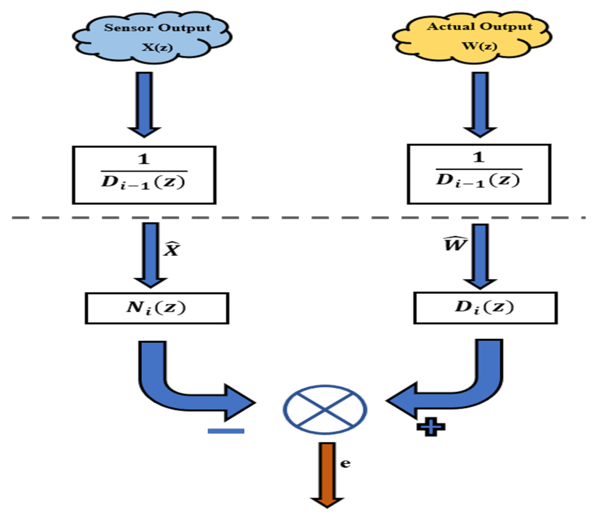
3. Data Fusion of the Sensors to the Actual Value

A load cell is placed under the receiver tank, and an actual mass flow rate is found. The linear modeling of the sensors is performed against the true value to find the correlation between the sensor output and the real value. Steiglitz-McBride et al.’s [24] iterative maximum likelihood algorithm co-relates the output of the electrical and mechanical sensor to the actual MFR. This technique is based on identifying and modeling a linear system. The system consists of the samples provided by its input and output in noise by reducing the mean square error. The transition function of the chosen model is a ratio of polynomials in $Z^{-1}$. Despite the fact that the regression equations for the optimum set of coefficients are strongly nonlinear and obstinate, it is shown that the problem can be minimized to recreate a solution of a similar linear problem [25]. The sensor’s output and the actual values relate by a rational z-transform, as shown in Equation (6) [26]:

$$\frac{Y\left(Z\right)}{U\left(Z\right)}=\frac{N\left(Z\right)}{D\left(Z\right)}$$

(6)

where $N\left(Z\right)={\alpha }_0+{\alpha }_1{Z}^{-1}+\dots +{\alpha }_{n-1}{z}^{-\left(n-1\right)}$ and $D\left(Z\right)=1+{\beta }_1{Z}^{-1}+\dots +{\beta }_n{z}^{-n}$.

If $x$ and $w$ are the finite histories of input and output samples, the mean squared error is given by:

$${\displaystyle \sum }{e}_j^2=\frac{1}{2\pi j}{\displaystyle \oint }{\left|XN-WD\right|}^2\frac{dz}{z}=min$$

(7)

where $X=X\left(z\right)=\sum x_j{z}^{-j}$ and $W=W\left(z\right)=\sum w_j{z}^{-j}$.

From Equation (7) [26], the mean square error between the sensor output and the system’s actual output is given as follows:

$${\displaystyle \sum }{e}_j^2=\frac{1}{2\pi j}{\displaystyle \oint }{\left|X\frac{N}{D}-W\right|}^2\frac{dz}{z}=min$$

(8)

Equation (8) [26] is a highly nonlinear regression problem. Steiglitz-McBride’s iterative technique minimizes the mean square error using linear regression, as shown in Equation (9) [27]. The procedure for minimizing error is graphically illustrated in Figure 2.

$${\displaystyle \oint }{\left|X\frac{N_i}{D_{i-1}}-W\frac{D_i}{D_{i-1}}\right|}^2\frac{dz}{z}={\displaystyle \oint }{\left|X\frac{N_i}{D_i}-W\right|}^2{\left|\frac{D_i}{D_{i-1}}\right|}^2\frac{dz}{z}=min$$

(9)

where $i=1,2,3\dots$ and $D_0=1$.

4. Solid Flow Simulation

According to the Euler–Lagrangian model, solid particles sliding on an inclined surface behave as discrete dense phases [26]. The fluid phase of air is a continuous medium, whereas the particle phase is discrete. There are three types of particle motion: immediate collision, particle momentum, and suspension motion, which are regulated by drag force. The Navier-Stokes (NS) equation [27] of the continuous medium explains the particle motion using the trajectory of every particle, which can be calculated using Equation (10) [27]:

$$\frac{d{u}_p}{dt}=F_D\left(u-u_p\right)+\frac{g_x\left({\rho }_p+\rho \right)}{{\rho }_p}+F_x$$

(10)

where $u_p$ is solid particle velocity, $u$ is the velocity of fluid-air, ${\rho }_p$ is the particle density, the density of the fluid is represented by $\rho$, and the gravity that influenced the particle is denoted as $g_x$. The three terms on the right-hand side of the equation explain the drag of the unit mass particle, the resultant of gravity, and the buoyant force [15,26], and the last term is a resultant force of other additional forces. The drag force, $F_D$, can be calculated using Equation (11) [27]. The correlation to calculate $C_D$ is given by Equation (12) [27].

$$F_D=\frac{3\mu C_{D}R{e}_p}{4{\rho }_P{d}_P^2}$$

(11)

$$C_D=a_1+\frac{a_2}{R{e}_P}+\frac{a_3}{R{e}_P^2}$$

(12)

where $a_1,a_{2,}{a}_3$are constants and $R{e}_P$ is the Reynolds number of the particle [27]. Another approach for multiphase flow is a two-fluid model in which each phase has different flow characteristics and considers a continuous medium. Both phases can penetrate one another, and the forces couple with the model based upon the Euler framework [28]. The continuity equation for the fluid phase is given by Equation (13) [28]:

$$\frac{\partial \left({\alpha }_q{\rho }_q\right)}{\partial t}+\nabla .\left({\alpha }_q{\rho }_q\overrightarrow{v_q}\right)={\displaystyle \sum }_{P=1}^n{\dot{m}}_{Pq}$$

(13)

where ${\alpha }_q$ is the volume fraction of phase $q$, ${\rho }_q$is the physical density of phase $q$, $\overrightarrow{v_q}$ is the speed of phase $q$, and ${\dot{m}}_{Pq}$ is the mass transfer flux from phase $p$ to phase $q$.

$$\frac{\partial \left({\alpha }_q{\rho }_q{\overrightarrow{V}}_q\right)}{\partial t}+\nabla .\left({\alpha }_q{\rho }_q\overrightarrow{V_q}\right)=-{\alpha }_q\nabla P+\nabla .\stackrel{=}{{\tau }_q}+{\displaystyle \sum }_{P=1}^n\left(\overrightarrow{R_{pq}}+{\dot{m}}_{pq}\overrightarrow{V_{pq}}\right)+{\alpha }_q{\rho }_q\left({\overrightarrow{F}}_q+\overrightarrow{F_{lift,q}}+\overrightarrow{F_{Vm,q}}\right)$$

(14)

where $\stackrel{=}{{\tau }_q}$ is the pressure strain tensor of phase $q$, ${\overrightarrow{F}}_q$is the external volume force, for the lifting force, ${\overrightarrow{F}}_{lift,q}$, and another force that plays its part is virtual mass force, $\overrightarrow{F_{Vm,q}}$. There is a force $\overrightarrow{R_{pq}}$ that is responsible for the interaction force between the phases, shred pressure is denoted as$P$ in all phases, and ${\overrightarrow{V}}_{pq}$ is the speed difference between the two phases [29].

4.1. Simulation Analysis

To simulate the flow of air-solid particles in a 3D rectangular inclined channel, ANSYS R16.0 FLUENT was used. The dimensions of the rectangular channel inclined at an angle of 50° were set as 1 × 2 × 33 cm³.

Table 1. Channel and solid particle values.

	Dimension/Property	Value
Channel	Length	33 cm
	Width	2 cm
Solid Particles	Height	1 cm
	Inclination	50°
	Density	2500 kg/m3
	Viscosity	0.001003 kg/m.s,
	Diameter	0.111 mm
	Packing limit	0.6
	Velocity	0.47 m/s

shows the characteristics of the solid particles and the simulation test channel. Initially, a coarser mesh of low resolution, later converted by a fine mesh, was created, with 569,121 nodes and 528,000 elements. The mesh was autogenerated and rectangular in shape. Since the channel was also rectangular, non-overlapping rectangular mesh elements of high resolution did not require any editing in the proposed structure. For modeling the flow of air-solid particles: steady-state, pressure-based, and under the influence of gravity, a multiphase Eulerian model with standard k-ε viscosity, standard wall function in the Near-Wall treatment list, and mixture in the Turbulence Multiphase Model list was used throughout the simulation. New material sand created a density of 2500 kg/m³, viscosity of 0.001003 kg/m.s, and a granular solid particle diameter size of 0.111 mm. The granular viscosity was selected, and granular bulk viscosity was set according to Rao et al. [30], while the packing limit was adjusted to 0.6 for phase interactions. The air and solid particles’ inlet speed was set at 0.47 m/s. The walls were assigned nonslip conditions. The inlet volume fraction of the granular solid particles is selected as 20%. The outlet boundary conditions were set at 100% outflow. The simulation ran for 1400 iterations, and the residuals converged to straight lines [31,32]. The inlet and outlet mass flow rates for the solid and the air are shown in

Table 2. Mass flow rate for sand and air.

	Measurement Points	Flow(kg/s)
Sand-MFR	Inlet	0.047
	Outlet	−0.06980251
	Net	−0.02280251
	Inlet	9.212002 × 10−05
Air-MFR	Outlet	−8.094581 × 10−05
	Net	1.1174421 × 10−05

. The sign conventions indicate the flow towards (+) and out of (−) the consideration plane.

4.2. Simulation Analysis

The pneumatically conveyed solid particles in a rectangular inclined channel were observed at two different planes, one in the center of the channel and one in the outlet. The volume fraction and velocity pattern of both air and solid particles were observed to investigate the flow pattern of the air-solid flow. The velocity and volume fraction of the air are evenly distributed at the inlet of the channel. The air velocity at the inlet is 0.47 m/s, and its volume fraction is 80%, which was evenly distributed.

The air velocity is significant in the dense phased solid particles region. Notably, in the location where the air and solid particles interact, the air molecules accelerate due to the flow of solid particles, and the velocity of 0.94 m/s exceeds the inlet velocity of 0.47 m/s. However, as it proceeds further towards the top wall, the velocity decreases, as shown in Figure 3. It is evident from Figure 4 that under the influence of gravity, the solid particle settles at the bottom wall. As a result, the significant portion of the plane occupied by the air volume fraction varies from 41% in the dense phased solid powder region to approximately 100% in the plane. The velocity and volume fraction profile of the solid particles at plane 2 is shown in Figure 5 and Figure 6, respectively. The concentration of the particles sliding in an inclined plane is maximum at the bottom surface, at 58.8%. The reason is the effect of gravity [33]. However, a negligibly low concentration of particles is suspended in the space of the plane. The velocity in the highly concentrated region is 0.73 m/s and further accelerates up to 0.95 m/s in the area of the air–solid interaction, as shown in Figure 6. Figure 7 and Figure 8 show the air velocity and volume fraction at the outlet, respectively. The volume concentration of the air at the bottom surface is 41.09%. The concentration in the rest of the plane is close to 100%. However, a regular, well-defined velocity pattern follows by air at the outlet. The velocity is maximum in the center, 0.89 m/s, and decreases as it moves upwards in the channel. Figure 9 and Figure 10 show the velocity and the volume fraction of sand particles in the outlet (sand particles act as solid particles in the given scenario). It is clear from Figure 10 that the volume fraction of sand particles along the lower surface is 58.91%. A negligibly low concentration of the solid particles is suspended in the remaining plane, which is carried away by air.

Similar to the air velocity profile, the solid particles also exhibit a well-defined regular pattern of the velocity profile, as shown in Figure 9. The region of the air–solid interaction offers the maximum velocity of 0.951 m/s. However, the suspended negligible small concentration of the particles shows a comparatively low velocity, as shown in Figure 9. Therefore, their impact on the mass flow rate measurement is ignorable since its concentration is too low. Numerical simulation of pneumatic flow is important to the visualization of solid flow [34]. Choking flow pipes and ducts because of cohesiveness is a big issue in the process industry [35,36]. Simulation results show the effect of gravity on the movement of the particles. However, the concentration of the suspended particles was low compared to the sliding particles at the bottom surface, but the moving air tends to suspend the solid particles. Based upon Figure 6 and Figure 10 from the simulation analysis, we observed that the volume fraction and the velocity of the solid particles do not remain constant along the z-axis. Instead of using a circular channel, a rectangular channel was used to ensure that all the velocity and volume fraction variations are within the upper and lower surface. Additionally, the electrodes of the electric sensors will be attached to the lower and upper surfaces to guarantee that particles must flow between the electrodes only [37].

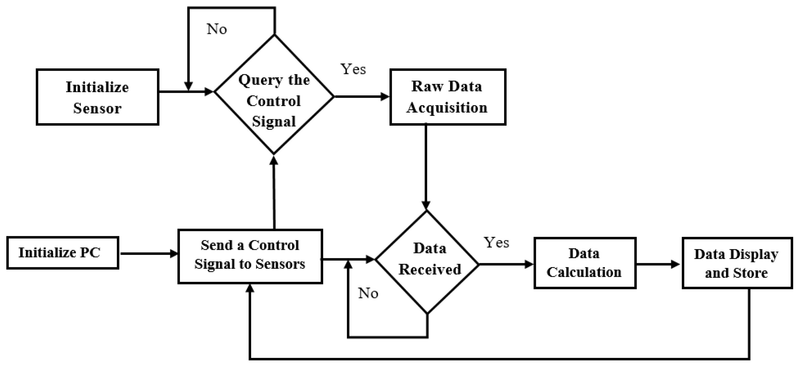
5. Measurement System

The MFR of pneumatically flowing solid particles is directly related to the MFR of the tapping line, which is directly related to the MFR of densely concentrated solid particles flowing down the inclined surface. Dilute phase flow measurement in terms of variations in capacitance is hard to trace. Hence, the air is removed, and the densely concentrated sample as a fraction of actual flow is measured, which affords substantial variations in capacitance values as solid particles flow through it [31]. This observable sensor section of the channel is not physically in direct contact with the rest of the system. In addition to that, two assumptions were ensured. First, the opening inlet aperture of the sensor channel is wide enough to accumulate all the incoming particles inside. Second, the air gap is at a minimum to avoid the variations in the load cell readings due to the hammering effect of the solid particles, which are presumed to be approximately zero [14].

The inclination angle of the observable channel is adjustable. It is set above the angle of repose to ensure all particles eventually slide down under gravity, and no layer exists permanently at the bottom. However, the velocity so obtained is an average value approximation. In real MFR, the velocity in the center is higher than the particles sliding along the bottom surface, observing more friction. Thus, the weighing system serves as a second, more precise measurement tool for the MFR.

Design of Instrument

Basically, there are three parts to the electrical capacitive sensor-based system. A sensor assembly, a data-gathering system, and a computer to store readings and for analysis are all required. The suggested measurement system is schematically depicted in Figure 1, with a rectangular channel with an upper and lower surface equipped with two capacitive sensors, one upstream and one downstream. The time-synchronized data collecting technique, as well as an algorithm for cross-correlation, enables the determination of particle velocity. Additionally, the upstream sensor is employed to determine the volumetric flow concentration. Both sensors have copper electrodes. Sensors 1 and 2 have a surface area of 2 × 2 and 2 × 1 cm², respectively. However, the electrodes are only 0.2 mm thick. The sensors are coupled to a 1 × 2 × 33 cm³ inclined rectangular channel that adjusts to the desired angle. The sensors’ centers are separated by 11.5 cm, as shown in Figure 11. To protect the electrodes from extraneous electromagnetic interference, they are encased in a metallic shield connected to the shared ground. The Eval-AD7746EBZ is a CDC, i.e., capacitance to digital converter, and is employed in conjunction with the Arduino interface for the sending and storing of capacitance values in an attached computer system [12,32].

It is a more accurate force sensor since the alloy-steel structure and unique dimensions of load cells contribute to their ability to withstand shock loads above its maximum measuring capability. The load cell is also protected from irreparable damage as a result of excessive loading. The load cell employed in the suggested design has a resolution of 1 g and can measure up to 500 g. Different measurement ranges are possible for load cells. However, there is a trade-off in terms of sensitivity. For the purpose of improving weight measurement accuracy, high-value strain gauges with accuracy flexions are employed. The load cell is affixed to a lower side of the channel under observation. Its use is to determine sand mass that exists along the channel’s length—the load cell is connected to the computer via the integrated circuit HX711. Load cell and capacitive sensors’ data are time-synchronized, allowing for accurate measurements [33]. Figure 12 illustrates the measurement technique’s flow chart. PC software, capacitive sensor circuits, and load cells initialize, and then a control signal is sent through microcontrollers to Eval-AD7746EBZ and HX711 simultaneously.

6. Results and Discussions

Many iterations of the experiment were performed to assess the efficacy of the multiple sensory arrangements that are suggested in this work. These iterations helped to choose the suitable distance between the electrodes, the dependency of the flow rate of the particles on the angle of inclination, and the range of the angle of inclination that generates a calculatable flow rate, since the instruments have a finite sampling rate. The channel is allowed to flow with bristlier dry sand with a typical particle diameter of 0.4 mm, a density of 2600 kg/m³, and a dielectric constant of less than or equal to 25, whereas less than or equal to 30 is tolerable to flow inside the channel. When the channel’s angle of repose-inclination was less than 50 degrees, the flow did not begin. The following parameters were calculated using data from electrical and mechanical sensors. Although the results obtained are very presentable, it was noted that sand particles in place of coal particles were used in experimental studies to reduce heap in the laboratory.

6.1. Design of Instrument

Capacitance values for the sensors were calculated as sand particles pass over the channel. Sensor 1 has an average value of 0.5229 pF, while sensor 2 has an average value of 0.4597 pF. Additionally, the amplitude of sensor 1’s variation in capacitance values is significantly greater than sensor 2’s variation in capacitance values [34]. While the rate of change remains the same, the pattern of variation in capacitance stays constant, consisting of a time delay. The difference of amplitude in mean readings and the variation of capacitive values are because sensor 1 is near twice the dimension of sensor 2. However, the comparison in the behavior indicates that whole sand flowing from the first sensor is likewise flowing with a temporal delay through the second sensor.

The normalized signals from the electric sensors are shown in Figure 13. Since for external electromagnetic interference, even with shielding, some noise is reduced by normalizing both signals, therefore, Equation (15) is used to normalize the electrical sensor output signals:

$$a{[n]}_{nor}=a\left[n\right]-\stackrel{\_\_\_\_\_}{a\left[n\right]}$$

(15)

where $\stackrel{\_\_\_\_\_}{a\left[n\right]}$ is the mean value of all output signal samples during the duration of the timeframe. The cross-correlation function between the normalized outputs of the sensors is calculated using Equation (2). A frame length of ±15 instants and a sample interval of 10 ms are used when setting the sampling rate.

The outcome of the cross-correlation of the normalized results of sensors 1 and 2 is shown in Figure 14. At the sixth instant, the greatest peak of the output signal arrives. As can be seen, the sand particles require an average of 60 milliseconds to move from sensor 1 to sensor 2. According to Equation (3), the velocity mean of the sand particles is 1.916 m/s.

6.2. Concentration of Volumetric Flow

Sand particle volumetric flow concentration is explained as a ratio of sand particle volume to the entire volume of the sensing zone during flow. The percentage (%) appears as an expression. The capacitive sensor must be calibrated initially to establish the link amongst the volumetric concentration and the capacitive measurements [35]. Determining the volume occupied by a particular mass involves finding the mass and density of the sand particles. Dividing it by a sensing region, total volume yields volumetric concentration data for a given mass of sand particles. A noted mass of sand particles presented amongst the parallel plates of sensor 1 is shown in

Table 3. Calibration parameters for average capacitance and volumetric concentration.

Capacitance (pF)	Mass (kg)	Volumetric Concentration (%)
0.49501	0	0
0.79612	0.0031	28.851
1.20063	0.0053	48.081
1.38101	0.0082	76.921
1.40193	0.0101	96.151

as mean capacitance values and volumetric concentration.

The MATLAB R2018a Curvefitting Tool (cftool) was employed to investigate a mathematical relation for volumetric concentration as a function of capacitive values using the calibration data presented in Equation (16):

$$\beta \left(c\right)=398.1c^3-1068c^2+969.1c-266.4$$

(16)

We used Equation (16) and the capacitance variation data from the first sensor for sand particles flowing through the channel, and calculated volumetric flow concentration of sand particles as shown in Figure 15. Only a very low concentration of sand particles (β < 10%) was present in the channel. For example, employing Equation (1) and values for ${\rho }_s$ = 2600 kg/m³, $A$ = 4 cm² (4 × 10⁴ m²), and $V_s\left(t\right)$ = 1.916 m/s (${\rho }_{s}A{V}_s\left(t\right)$ = K = 1.9844 kg/s), the MFR is given by Equation (17):

$$M\left(t\right)\cong K\beta \left(t\right)$$

(17)

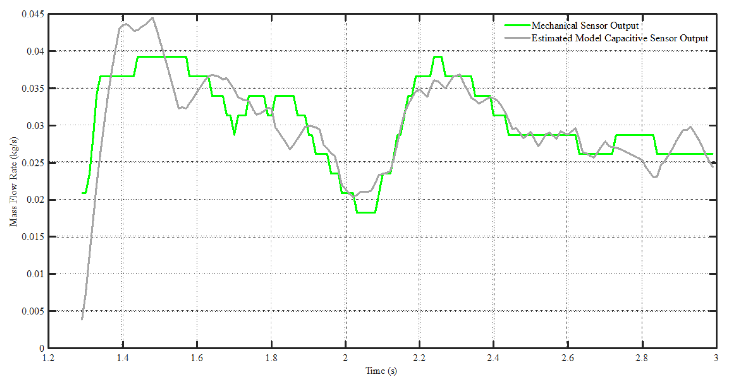
6.3. Measurements of Mechanical Sensor

The MFR measurement was obtained by plugging Equation (5) into the load cell. It is critical to note here that the MFR obtained from Equation (5) is an approximation of the average value at the channel’s cross-section. Its accuracy is based on the length of the channel being observed, which might vary widely.

Employing electrical and mechanical sensors both at the same time, Figure 16 compares the MFR measurement for the specific flow of sand particles from a channel. It is interesting to observe that the capacitor sensor assembly exhibits many variances. Among the specific reasons is the presence of a low-level noise signal during the concentration measurement. Another thing to remember is that the volume of the under-examination region is quite trivial. Thus, the constantly varying volume fraction of sand particles instils concentration variations that ultimately result in changes in MFR measurements [36,37]. However, the mechanical sensor’s results are relatively consistent. The reason for this is due to the small resolution of the load cell measurement and the mass being averaged across the channel length. The velocity utilized to calculate the MFR using a mechanical sensor is also derived from the capacitive sensor component.

At the initial start of the flow, the results cannot be in the same range because the electrical sensor measures instantaneously as the sand particles flow through it, as shown in Figure 16. However, the load cell reading is built up as the sand particles start filling up the length of the channel. Once it is filled up, the results become of the same range. By reducing the length of the channel, the load cell measurement results for MFR should be improved [38]. However, shortening the distance between electrical sensors may result in signal interference. Regarding the length of the channel, there will always be a compromise with the accuracy of both the sensors.

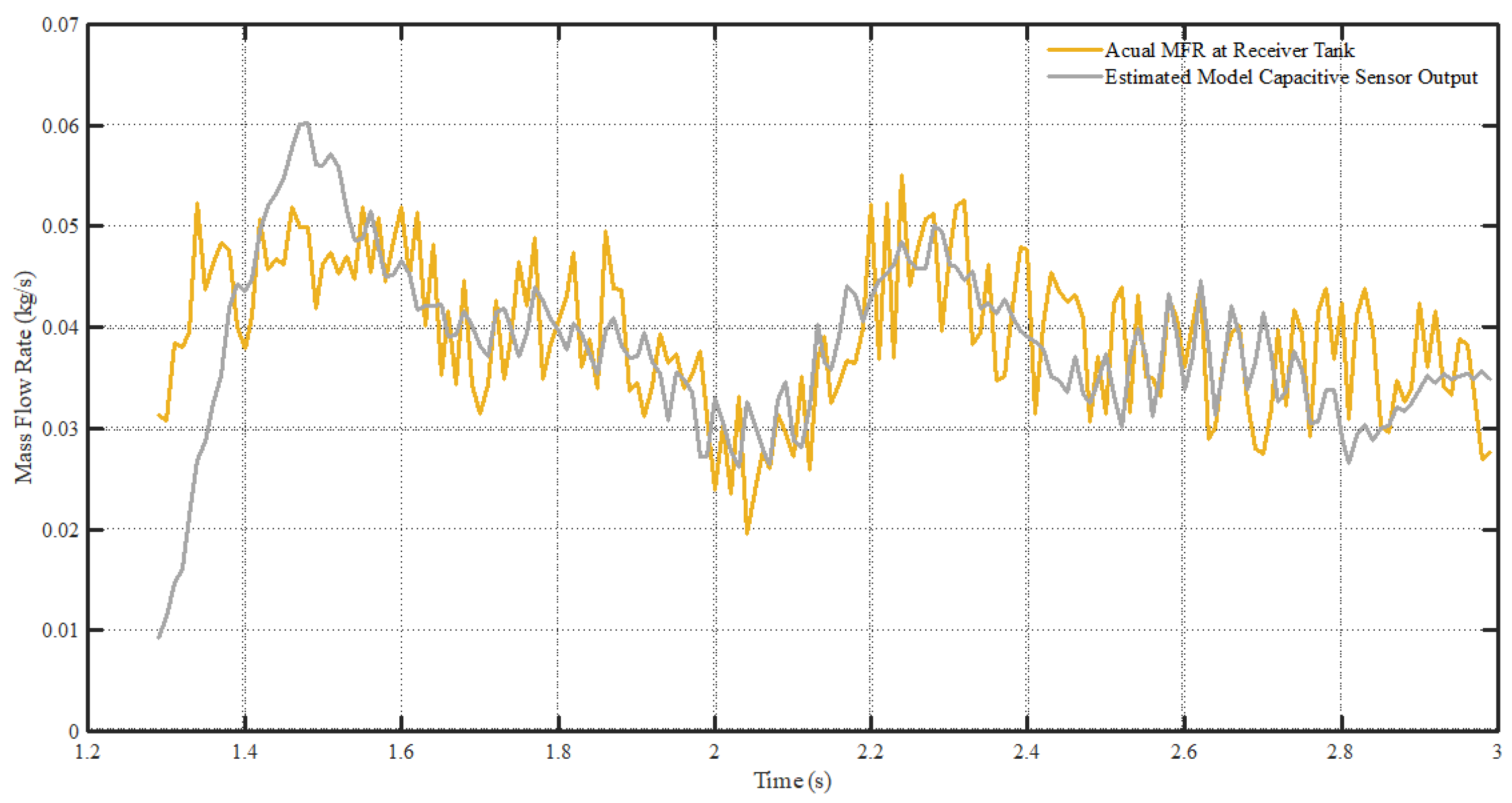
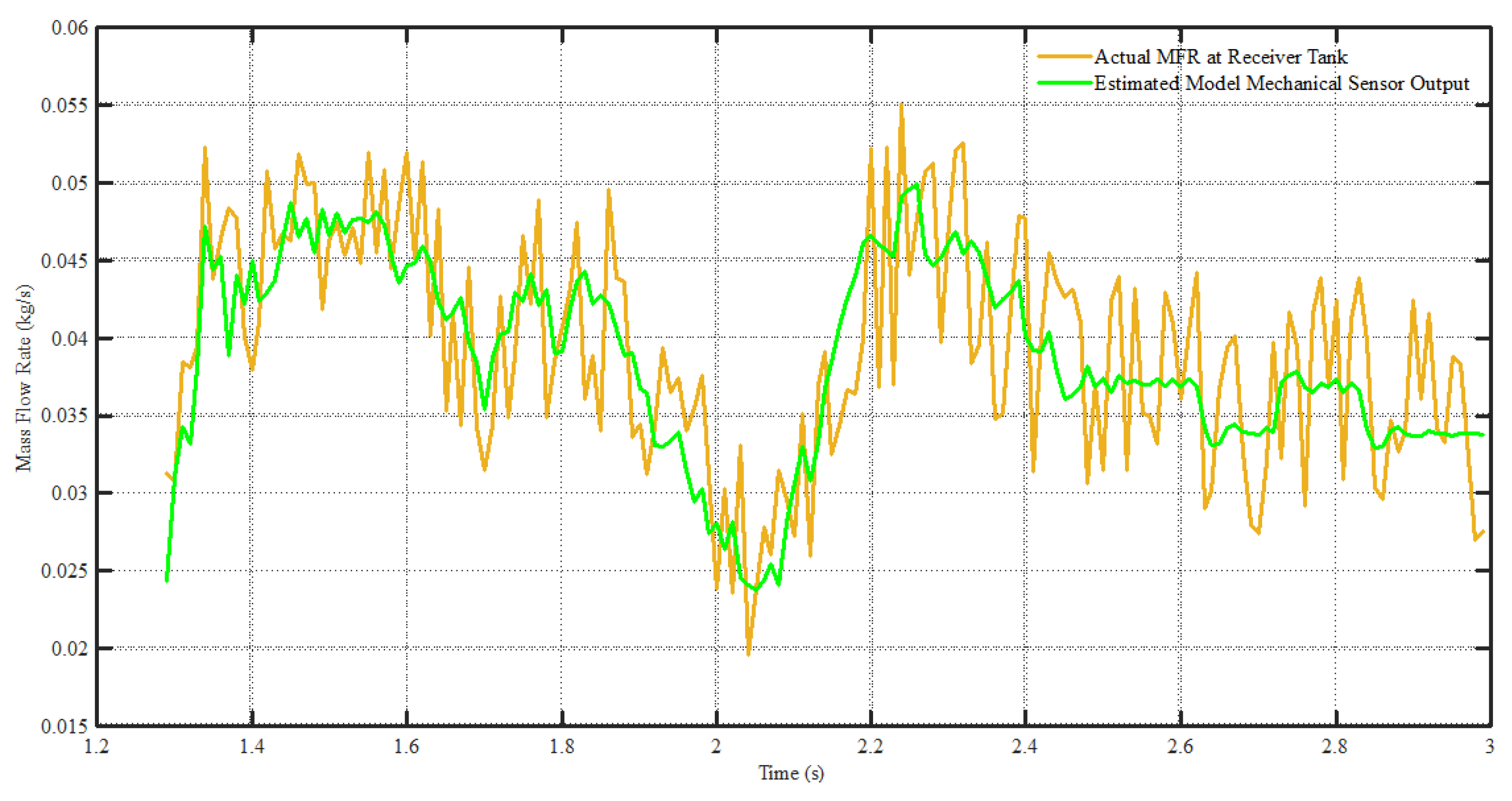
6.4. Data Fusion of Sensors to the Real MFR

A load cell is placed under the receiver tank to calculate the actual MFR. The data from all three sensors are time-synchronized. Figure 17 shows the MFR from an electrical sensor, mechanical sensor, and actual value.

The MFR at the outlet computed in the simulation was −0.06980251, as shown in Table 2. This numerical value is in accordance with real-time experimental results of MFR of the electrical sensor, mechanical sensor, and actual values shown in Figure 17. The MFR values in Figure 17 are between 0.04 and 0.07. The negative sign of the simulation result explains the direction of flow, i.e., outwards. Hence, the simulation results are validated by the experimental results of this research work.

Using Equations (6) and (9), the relationship between the sensors and the relationship between the real MFR $M_A\left(z\right)$ and the sensor’s output was found using MATLAB R2018a. The linear modeling between the electrical, $M_C\left(z\right),$and mechanical sensor, $M_M\left(z\right),$ outputs using Steiglitz-McBride’s iteration is given by Equation (18) and is shown in Figure 18.

$$M_M\left(z\right)\left[1-5.75 Z^{-1}+14.04Z^{-2}-19.12Z^{-3}+16.31Z^{-4}-9.68Z^{-5}+4.46Z^{-6}-1.54Z^{-7}+0.27Z^{-8}\right]=M_C\left(z\right)\left[0.1004-0.47Z^{-1}+0.90Z^{-2}-0.87Z^{-3}+0.42Z^{-4}-0.08Z^{-5}\right]$$

(18)

It is essential to mention here that only the steady flow of sand particles considered the initial few (130) samples of the data ignored when the output of the mechanical sensor was rising, because the channel did not fill with sand particles.

The actual MFR, $M_A\left(z\right)$, modeled as electrical sensor MFR output, $M_C\left(z\right)$, is shown in Figure 19, and the relationship between them is given by Equation (19):

$$M_A\left(z\right)\left[1-2.25 Z^{-1}+0.834Z^{-2}+1.23Z^{-3}-1.59Z^{-4}+1.28Z^{-5}+0.37Z^{-6}-1.65Z^{-7}+0.76Z^{-8}\right]=M_C\left(z\right)\left[0.21-0.41Z^{-1}+0.05Z^{-2}+0.30Z^{-3}-0.15Z^{-4}\right]$$

(19)

Similarly, the actual MFR, $M_A\left(z\right)$, modeled as mechanical sensor MFR output, $M_M\left(z\right)$, is shown in Figure 20, and the relationship between them is given by Equation (20):

$$M_A\left(z\right)\left[1-0.44Z^{-1}-0.58Z^{-2}+0.63Z^{-3}-0.39Z^{-4}-0.36Z^{-5}+0.39Z^{-6}-0.17Z^{-7}\right]=M_M\left(z\right)\left[1.17-0.20Z^{-1}-0.82Z^{-2}+0.16Z^{-3}-0.22Z^{-4}\right]$$

(20)

Figure 20 correlates actual MFR values with the mechanical sensor and capacitor sensor. In the case of mechanical sensors, the changes in the readings are very slow, so in order to model the mechanical sensor value to the real value, it required previous samples of both the mechanical sensor and real values in order to minimize the error through an iterative process. However, the variation in the electrical sensor values is quite frequent, in accordance with the real values, but is accompanied by external noise/disturbance, as shown in Figure 19. The iterative error reduction process required previous samples of both real values and sensor values to predict the current sensor value closer to the actual value with the least possible error.

7. Conclusions

This work used electrical and mechanical sensors to demonstrate the instrumentation system used to measure the flow of sand in the channel. The instrument system was designed to deal with many well-known problems related to measuring the MFR of pulverized coal in furnaces. Using electrical and mechanical sensors with hardware and software components, the results were quantifiable and comparable. The calibration of the mass flow load cell was performed on an autonomous load cell that measures the collective mass in the receiving tank during a specified time period. It is also important to emphasize that mechanical and electrical sensors complement each other by compensating for each other’s limitations. When sand particles pass through the air pneumatically, the mass of suspended particles is not visible on the load cell connected to the bottom of the channel. Therefore, in this case, the data of the electronic sensor will be more accurate. Therefore, if the sand particles are not uniform, the fluctuation of the capacitance cannot be used to estimate the flow concentration, since the non-uniformity of the sand has no effect on the MFR measurement based on the load cell. Nevertheless, the results of this study confirmed that the design has the potential to be suitable for the intended application field.

References

1. Cui, H.; Grace, J.R. Pneumatic Conveying of Biomass Particles: A Review. China Particuology 2006, 4, 183–188. [Google Scholar] [CrossRef]
2. Xie, H.; Tan, L.; Liu, J.; Chen, H.; Yang, H. Numerical and Experimental Investigation on Opening Direction Steady Axial Flow Force Compensation of Converged Flow Cartridge Proportional Valve. Flow Meas. Instrum. 2018, 62, 123–134. [Google Scholar] [CrossRef]
3. Tominaga, Y.; Okaze, T.; Mochida, A. Wind Tunnel Experiment and CFD Analysis of Sand Erosion/Deposition Due to Wind around an Obstacle. J. Wind Eng. Ind. Aerodyn. 2018, 182, 262–271. [Google Scholar] [CrossRef]
4. Zheng, Y.; Liu, Q. Review of Techniques for the Mass Flow Rate Measurement of Pneumatically Conveyed Solids. Meas. J. Int. Meas. Confed. 2011, 44, 589–604. [Google Scholar] [CrossRef]
5. Sen, S.; Das, P.K.; Dutta, P.K.; Maity, B.; Chaudhuri, S.; Mandal, C.; Roy, S.K. PC-Based Gas-Solids Two-Phase Mass Flowmeter for Pneumatically Conveying Systems. Flow Meas. Instrum. 2000, 11, 205–212. [Google Scholar] [CrossRef]
6. Zhang, W.; Wang, C.; Yang, W.; Wang, C.H. Application of Electrical Capacitance Tomography in Particulate Process Measurement—A Review. Adv. Powder Technol. 2014, 25, 174–188. [Google Scholar] [CrossRef]
7. McKee, S.L.; Dyakowski, T.; Williams, R.A.; Bell, T.A.; Allen, T. Solids Flow Imaging and Attrition Studies in a Pneumatic Conveyor. Powder Technol. 1995, 82, 105–113. [Google Scholar] [CrossRef]
8. Xia, H.; Kan, R.; Xu, Z.; He, Y.; Liu, J.; Chen, B.; Yang, C.; Yao, L.; Wei, M.; Zhang, G. Two-Step Tomographic Reconstructions of Temperature and Species Concentration in a Flame Based on Laser Absorption Measurements with a Rotation Platform. Opt. Lasers Eng. 2017, 90, 10–18. [Google Scholar] [CrossRef]
9. Hu, H.L.; Xu, T.M.; Hui, S.E.; Zhou, Q.L. A Novel Capacitive System for the Concentration Measurement of Pneumatically Conveyed Pulverized Fuel at Power Stations. Flow Meas. Instrum. 2006, 17, 87–92. [Google Scholar] [CrossRef]
10. Ismail, B.; Ahmed, W. Innovative Techniques For Two-Phase Flow Measurements. Recent Patents Electr. Eng. 2010, 1, 1–13. [Google Scholar] [CrossRef]
11. Holler, G.; Fuchs, A.; Hrach, D. Flow Velocity Determination in Cryogenic Media by Means of Capacitive Sensing. In Proceedings of the 3rd International Conference on Sensing Technology, Taipei, Taiwan, 30 November–3 December 2008; pp. 472–476. [Google Scholar]
12. Brasseur, G.; Brandstätter, B.; Zangl, H. State of the Art of Robust Capacitive Sensors. In Proceedings of the 1st International Workshop on Robotic Sensing, 2003, ROSE’ 03, Oorebo, Sweden, 3–6 October 2003. [Google Scholar]
13. Bretterklieber, T.; Zangl, H.; Holler, G.; Hrach, D.; Hammerschmidt, D.; Motz, M. Vielseitig Anwendbare Auswerteeinheit Für Robuste Kapazitive Sensoren. Elektrotechnik Inf. 2008, 125, 132–137. [Google Scholar] [CrossRef]
14. Sun, M.; Liu, S.; Lei, J.; Li, Z. Mass Flow Measurement of Pneumatically Conveyed Solids Using Electrical Capacitance Tomography. Meas. Sci. Technol. 2008, 19, 19. [Google Scholar] [CrossRef]
15. Abrar, U.; Shi, L.; Jaffri, N.R.; Short, M.; Hasham, K. Electrical and Mechanical Sensor-Based Mass Flow Rate Measurement System: A Comparative Approach. In Proceedings of the 2020 4th International Conference on Robotics and Automation Sciences (ICRAS), Wuhan, China, 12–14 June 2020; IEEE: Wuhan, China, 2020. [Google Scholar]
16. Zheng, Y.; Liu, Q. Review of Certain Key Issues in Indirect Measurements of the Mass Flow Rate of Solids in Pneumatic Conveying Pipelines. Measurement 2010, 43, 727–734. [Google Scholar] [CrossRef]
17. Yan, Y.; Byrne, B.; Woodhead, S.; Coulthard, J. Velocity Measurement of Pneumatically Conveyed Solids Using Electrodynamic Sensors. Meas. Sci. Technol. 1995, 6, 515–537. [Google Scholar] [CrossRef]
18. Zhang, W.; Wang, C.; Wang, Y. Parameter Selection in Cross-Correlation-Based Velocimetry Using Circular Electrostatic Sensors. IEEE Trans. Instrum. Meas. 2010, 59, 1268–1275. [Google Scholar] [CrossRef]
19. Ortmanns, M.; Buhmann, A.; Manoli, Y.; Achour, H. Interface Circuits. In Reference Module in Materials Science and Materials Engineering; Elsevier: Amsterdam, The Netherlands, 2016. [Google Scholar]
20. Zhang, M.; Ma, L.; Soleimani, M. Magnetic Induction Tomography Guided Electrical Capacitance Tomography Imaging with Grounded Conductors. Meas. J. Int. Meas. Confed. 2014, 53, 171–181. [Google Scholar] [CrossRef] [Green Version]
21. Jaffri, N.R.; Almogren, A.; Ahmad, A.; Abrar, U.; Radwan, A.; Khan, F.A. Iterative Algorithms for Deblurring of Images in Case of Electrical Capacitance Tomography. Math. Probl. Eng. 2021, 2021, 1–11. [Google Scholar] [CrossRef]
22. Gajewski, J.B. Electrostatic Nonintrusive Method for Measuring the Electric Charge, Mass Flow Rate, and Velocity of Particulates in the Two-Phase Gas-Solid Pipe Flows–Its Only or as Many as 50 Years of Historical Evolution. IEEE Trans. Ind. Appl. 2008, 44, 1418–1430. [Google Scholar] [CrossRef]
23. Li, J.; Fu, F.; Li, S.; Xu, C.; Wang, S. Velocity Characterization of Dense Phase Pneumatically Conveyed Solid Particles in Horizontal Pipeline through an Integrated Electrostatic Sensor. Int. J. Multiph. Flow 2015, 76, 198–211. [Google Scholar] [CrossRef]
24. Steiglitz, K.; McBride, L. A Technique for the Identification of Linear Systems. IEEE Trans. Automat. Contr. 1965, 10, 461–464. [Google Scholar] [CrossRef]
25. Jia, Y.; Chernyshev, V.; Skliar, M. Ultrasound Measurements of Segmental Temperature Distribution in Solids: Method and Its High-Temperature Validation. Ultrasonics 2016, 66, 91–102. [Google Scholar] [CrossRef] [Green Version]
26. Zhang, S.; Chen, L.; Meng, Z.; Zhang, G. Numerical Research of Magnetohydrodynamics Buoyant Flow in Dual Functional Lead Lithium Fusion Blanket. Fusion Eng. Des. 2019, 149, 111331. [Google Scholar] [CrossRef]
27. Zhao, Y.; Wang, Y.; Yao, J.; Fairweather, M. Reynolds Number Dependence of Particle Resuspension in Turbulent Duct Flows. Chem. Eng. Sci. 2018, 187, 33–51. [Google Scholar] [CrossRef]
28. Gerber, S.; Oevermann, M. A Two Dimensional Euler–Lagrangian Model of Wood Gasification in a Charcoal Bed—Part I: Model Description and Base Scenario. Fuel 2014, 115, 385–400. [Google Scholar] [CrossRef]
29. Pietrzak, M.; Płaczek, M. Void Fraction Predictive Methods in Two-Phase Flow across a Small Diameter Channel. Int. J. Multiph. Flow 2019, 121, 103115. [Google Scholar] [CrossRef]
30. Rao, S.M.; Zhu, K.; Wang, C.H.; Sundaresan, S. Electrical Capacitance Tomography Measurements on the Pneumatic Conveying of Solids. Ind. Eng. Chem. Res. 2001, 40, 4216–4226. [Google Scholar] [CrossRef]
31. Orak, İ.; Koçyiğit, A. The Thickness Effect of Insulator Layer between the Semiconductor and Metal Contact on C-V Characteristics of Al/Si3N4/p-Si Device. Pamukkale Univ. J. Eng. Sci. 2017, 23, 536–542. [Google Scholar] [CrossRef] [Green Version]
32. Huang, Z.; Zhu, J.; Lu, L. An AD7746-Based Data Acquisition System for Capacitive Pressure Sensor in Weather Detection Application. Key Eng. Mater. 2011, 483, 461–464. [Google Scholar] [CrossRef]
33. Che, H.Q.; Wu, M.; Ye, J.M.; Yang, W.Q.; Wang, H.G. Monitoring a Lab-Scale Wurster Type Fluidized Bed Process by Electrical Capacitance Tomography. Flow Meas. Instrum. 2018, 62, 223–234. [Google Scholar] [CrossRef] [Green Version]
34. Xul, L.; Carter, R.M.; Yan, Y. Mass Flow Measurement of Fine Particles in a Pneumatic Suspension Using Electrostatic Sensing and Neural Network Techniques. In Proceedings of the 2005 IEEE Instrumentationand Measurement Technology Conference Proceedings, Ottawa, ON, Canada, 16–19 May 2005; pp. 17–19. [Google Scholar]
35. Szpica, D. The Determination of the Flow Characteristics of a Low-Pressure Vapor-Phase Injector with a Dynamic Method. Flow Meas. Instrum. 2018, 62, 44–55. [Google Scholar] [CrossRef]
36. Yan, Y. Mass Flow Measurement of Bulk Solids in Pneumatic Pipelines. Meas. Sci. Technol. 1996, 7, 1687–1706. [Google Scholar] [CrossRef]
37. Gagliano, S.; Stella, G.; Bucolo, M. Real-Time Detection of Slug Velocity in Microchannels. Micromachines 2020, 11, 241. [Google Scholar] [CrossRef] [PubMed] [Green Version]
38. Klinzing, G.E. Historical Review of Pneumatic Conveying. Kona Powder Part. J. 2018, 2018, 150–159. [Google Scholar] [CrossRef] [Green Version]
Figure 1. Experimental setup for this research.
Electronics 10 02849 g001
Figure 2. Iterative procedure for minimizing error.
Electronics 10 02849 g002
Figure 3. Air velocity at plane 2.
Electronics 10 02849 g003
Figure 4. Air volume fraction at plane 2.
Electronics 10 02849 g004
Figure 5. Sand velocity at plane 2.
Electronics 10 02849 g005
Figure 6. Sand volume fraction at plane 2.
Electronics 10 02849 g006
Figure 7. Air velocity at the outlet.
Electronics 10 02849 g007
Figure 8. Air volume fraction at the outlet.
Electronics 10 02849 g008
Figure 9. Sand velocity at the outlet.
Electronics 10 02849 g009
Figure 10. Sand volume fraction at the outlet.
Electronics 10 02849 g010
Figure 11. (a) Channel for solid particle flow. (b) Actual capacitive electrodes for the experimental setup.
Electronics 10 02849 g011
Figure 12. Flow chart to explain sensor data acquisition system layout.
Electronics 10 02849 g012
Figure 13. The normalized output of electric sensors.
Electronics 10 02849 g013
Figure 14. Cross-correlation between two electric sensors.
Electronics 10 02849 g014
Figure 15. Volumetric flow concentration of sand particles using an electric sensor.
Electronics 10 02849 g015
Figure 16. MFR of sand particles measured by electrical and mechanical sensors.
Electronics 10 02849 g016
Figure 17. MFR from the electrical sensor, mechanical sensor, and actual value.
Electronics 10 02849 g017
Figure 18. MFR mechanical sensor as a function of MFR capacitive sensor.
Electronics 10 02849 g018
Figure 19. Actual MFR as a function of the MFR capacitive sensor.
Electronics 10 02849 g019
Figure 20. Actual MFR as a function of the MFR mechanical sensor.
Electronics 10 02849 g020