Output-Based Tracking Control for a Class of Car-Like Mobile Robot Subject to Slipping and Skidding Using Event-Triggered Mechanism

Abstract

This paper presents an output-based tracking controller for a class of car-like mobile robot (CLMR) subject to slipping and skidding. The slipping and skidding are regarded as external disturbances, and an event-triggered extended state observer (ET-ESO) is utilized to recover the velocities as well as to estimate the uncertainties and disturbances. The constrained longitudinal velocity is established, conforming to the traffic flow theory on the kinematic level. The velocity control law and heading angle control law are developed on the dynamic level, respectively. The input to state stability (ISS) of the closed-loop system is analyzed via cascade theory. Simulation results are given to demonstrate the effectiveness of the proposed tracking controller for CLMR subject to slipping and skidding.

1. Introduction

With the increasingly widespread application of robotics, wheeled mobile robots (WMRs) tracking control problems have been studied in the past two decades. Automatic braking, adaptive cruise control and platooning control of intelligent connected vehicle have attracted the attention of many researchers, while stability and control performance are the prerequisites for practical tasks, such as farm vehicles, logistics transportation, search and rescue, hospital tasks and so on [1,2,3,4,5,6,7,8].

A variety of control strategies is utilized to achieve optimized performance. In [7,8,9,10], path following and tracking control schemes were respectively developed for CLMRs and four-wheeled WMR by using the back-stepping method. In order to obtain the global optimal solution, neural-dynamic online optimization-based model predictive control (MPC) schemes were presented for the path tracking problem and formation control of CLMR in [11,12]. In [13,14], hierarchical fuzzy decentralized sliding mode controllers (SMCs) were developed for the CLMR trajectory tracking, where the mathematical model was no longer required and the motor dynamics were sufficiently considered in the controller design. The model uncertainties and external disturbances were estimated by using linear ESO and compensated on the kinetic level. It is worth noting that the conditions of non-skidding and non-slipping should be satisfied in the aforementioned result [9,10,11,13,14]. However, the assumptions cannot be met when the CLMR works in the environments, such as on the icy roads, the wet roads, and the forestry roads. The stability and performance may consequently no longer be guaranteed. To address the slipping and skidding problem, tracking controllers were presented for WMRs with longitudinal and lateral slippage based on improved linear active disturbance rejection control (ADRC) in [15], a disturbance observer in [16] and the reinforcement learning method in [17]. In the existing results [12,15,16,17], the virtual velocity input or given velocity is unlimited, which means that negative longitudinal velocity may come out during movement. Noting that it violates the traffic flow theory in the application of WMRs such as logistics system and self-driving automobile, which intensifies the potential collision risk, it is highly desirable to develop a tracking control scheme with velocity constraints.

Another challenge in the tracking control of CLMR is to obtain the desired performance with the least resources in the presence of model uncertainties and disturbances, including least sensors and communication bandwidth. In [7,8], skidding and slipping were handled as input-additive and unmatched perturbations of kinematics and dynamics. The CLMR’s posture, velocities and perturbations were measured by using a real-time kinematic global positioning system (RTK-GPS) and other aiding sensors. ESOs were widely adopted to estimate the total disturbances recently. In [18], a robust tracking controller was proposed for Type (2,0) WMR with unknown skidding and slipping by using a generalized ESO approach. In [19,20,21,22,23,24,25,26,27,28], output feedback-based control schemes were established for autonomous surface vehicles. ESOs were utilized to recover the unknown velocities and to estimate the total disturbances as well as the unavailable sideslip angle. In [29,30], event-triggered ESOs were utilized to recover the dynamic positioning vessels velocities and the total disturbances from position-heading sensors, such as GNSS and the inertial measurement unit. Since the measurements were transmitted only at the event-triggered instants, the sensor-to-observer communication is remarkably reduced. From a practical perspective, it is rewarding to investigate the tracking control of CLMR with skidding and slipping based on the output information and event-triggered mechanism.

Based on the above observations, this paper considers the constrained tracking control for a class of CLMR subject to slipping and skidding. The slipping and skidding are regarded as external disturbances, and an ET-ESO is utilized to recover the velocities as well as to estimate the uncertainties and disturbances. Longitudinal velocity is established conforming to the traffic flow theory on the kinematic level. The velocity control law and heading angle control law are subsequently developed on the dynamic level. Simulation results are given to demonstrate the effectiveness of the proposed tracking controller for CLMRs subject to slipping and skidding. The main contributions of the proposed constrained tracking control scheme are outlined as follows. (1) In contrast to the GPS-based control scheme in [7,8] and neural-network-based control scheme in [12,17], the proposed control scheme is more efficient to implement in practical application. Especially, with the proposed ET-ESO, the velocity can be recovered, and the disturbances can be compensated in the presence of skidding and slipping. (2) In contrast to the robust tracking controller in [7,12,15,16], the constrained longitudinal velocity is established, conforming to the traffic flow theory, and negative velocity can be avoided, which is very significant for energy saving and safety in some applications. (3) In contrast to the tracking control in [13,14,15,16], a dynamic controller is also involved in the proposed output-based tracking controller for CLMR.

The remainder of this paper is organized as follows. Section 2 presents some preliminaries and the problem formulation. The development of an ESO-based controller is described in Section 3. Section 4 provides analysis for the cascade close-loop system. Section 5 gives an example for illustrations. Section 6 concludes the paper.

Throughout the paper, ${\Re }^{m\times n}$ denotes the set of all $m\times n$ real matrices. $∥·∥$ denotes the Euclidean norm, ${\lambda }_{min}(·)$, and ${\lambda }_{max}(·)$ denote the minimum and maximum eigenvalues of a matrix, respectively.

2. Preliminaries and Problem Formulation

2.1. Dynamic Model of CLMR

CLMRs are widely adopted in complicated working conditions, such as heavy-load transport and uneven pavement surface. Considering the kinematic perturbations caused by wheel slipping and skidding [7,8], the kinematic model of CLMR shown in Figure 1 is generally described as follows:

$$\left\{\begin{array}{c}\dot{p}=J\left(\psi \right)v,\hfill \\ \dot{\psi }=[\frac{tan(\theta +{\delta }_1)}{L},\frac{-1}{L}]v,\hfill \\ \dot{\theta }=\omega ,\hfill \end{array}\right.$$

(1)

where $p={[x,y]}^T\in {\Re }^2$ denotes the CLMR’s position in the global frame; $\psi \in \Re$ denotes the CLMR’s heading angle;

$$J\left(\psi \right)=\left[\begin{array}{cc}cos\left(\psi \right)& -sin\left(\psi \right)\\ sin\left(\psi \right)& cos\left(\psi \right)\end{array}\right],$$

is the rotation matrix; $v={[v_x,v_y]}^T\in {\Re }^2$ denotes the velocity vector consisting of the longitudinal linear velocity $v_x$ and lateral velocity $v_y$; $L\in \Re$ denotes the CLMR’s wheelbase; $\theta \in \Re$ denotes the CLMR’s front steering angle; $\omega \in \Re$ denotes the rotational velocity of the front steering wheel; and ${\delta }_1\in \Re$ denotes the front slip angle.

The kinematic perturbations due to wheel skidding and slipping are characterized by $\{{\delta }_1,v_y,{\delta }_v\}$ with the following relations:

$$\left\{\begin{array}{c}{\delta }_2=arctan{v}_y/v_x,\hfill \\ v_x=r_w{\omega }_w-{\delta }_v,\hfill \end{array}\right.$$

(2)

where ${\delta }_2\in \Re$ denotes the rear slip angle, ${\delta }_v\in \Re$ denotes the longitudinal slip velocity, $r_w\in \Re$ denotes the radius of rear wheel, and ${\omega }_w\in \Re$ denotes the rotational velocity of rear wheel. The perturbations $\{{\delta }_1,v_y,{\delta }_v\}$ can be classified as follows: (1) ${\delta }_1$ and ${\delta }_v$ are input additive, and (2) $v_y$ is unmatched.

The dynamic of CLMR with the Euler–Lagrange formalism is subsequently given by the body velocity equation:

$$\dot{v}=M^{-1}{\tau }_v+g_v,$$

(3)

and the following steering wheel rotation equation:

$$\dot{\omega }=J_w^{-1}{\tau }_w+g_w,$$

(4)

where $M=diag\{m,m\}\in {\Re }^{2\times 2}$, and $m\in \Re$ denotes the mass of CLMR; $g_v={[g_{vx},g_{vy}]}^T=-C(p,v)v-G\left(p\right)+{\tau }_{dv}$, $C(p,v)\in {\Re }^{2\times 2}$ denotes the Coriolis, centrifugal and damping matrix in total; $G\left(p\right)\in {\Re }^2$ denotes the gravitational vector; ${\tau }_{dv}\in {\Re }^2$ denotes the nonlinear term with uncertainties and external disturbances; $J_w\in \Re$ denotes the front wheel’s moment of inertia; and ${\tau }_v={[{\tau }_x,{\tau }_y]}^T\in {\Re }^2$ and ${\tau }_w\in \Re$ denote the input vector for linear movement and wheel rotation, respectively.

For the reference point $p_r={[x_r,y_r]}^T$ on the trajectory, the tracking errors are defined as

$$\left\{\begin{array}{c}{e}_x=x-x_r,\hfill \\ e_y=y-y_r.\hfill \end{array}\right.$$

(5)

Noting that the lateral input force is unmatched, due to the under-actuated characteristic of CLMR, it can only be stabilized by developing kinematic control laws $[v_x,\theta ]$, and the input force satisfies ${\tau }_y=0$. According to the controller design and analysis in [18], an assumption is stated as follows.

Assumption 1.

The derivatives of $g_v$ and $g_w$ are bounded, such that $∥g_v∥+\left|g_w\right|\le g\ast$ with $g\ast \in \Re$ being a positive constant.

2.2. Control Objective

On one hand, the position-heading information is globally measured by global sensors such as the Beidou navigation positioning system integrated with the inertial measurement unit (IMU) or the simultaneous localization and mapping (SLAM) in most practical applications. Considering the fact that the slipping and skidding cannot be precisely measured, it is necessary to develop a tracking controller for CLMRs by using the output feedback method. On the other hand, the longitudinal velocity should be non-negative during the movement according to traffic flow theory, especially for the platoon control of CLMRs.

The control objective is to develop an output feedback-based controller for the CLMRs with (1), (3) and (4), such that the following hold:

(1) The CLMR is driven to track a given trajectory even when slipping occurs, i.e., $\underset{t\to \infty }{lim}∥p-p_r∥\le {\sigma }_1$;

(2) The CLMR moves at the desired velocity even when skidding occurs, and negative velocity should be avoided, i.e., $\underset{t\to \infty }{lim}\left|v-v_r\right|\le {\sigma }_2$ and $v_x\ge 0$;

(3) Both the unmeasured velocities v and the total disturbances are recovered by using the measured position-heading information, and the sensor-to-controller communication times should be distinctly reduced while retaining acceptable performance.

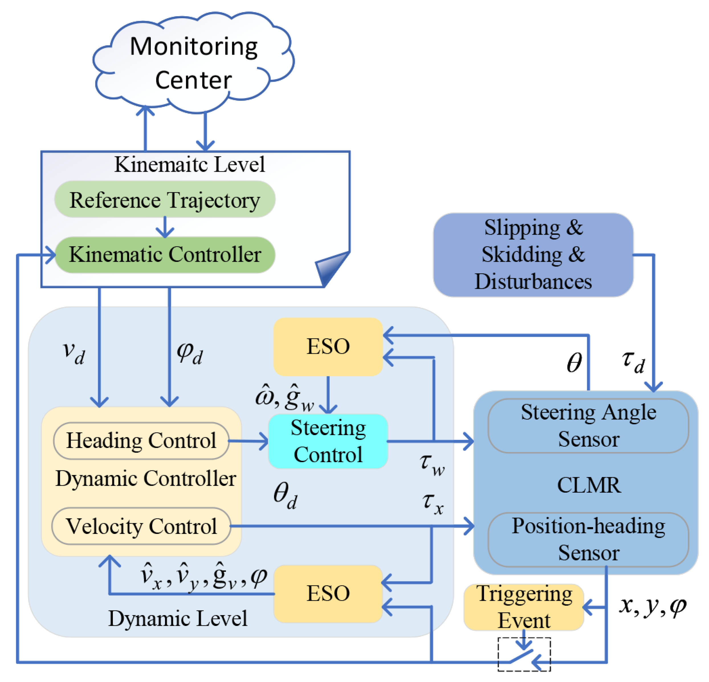
3. Controller Design

Control laws are established for velocity and heading, respectively, in this section. The scheme diagram of the proposed controller is depicted in Figure 2.

3.1. Kinematic Controller for Position

The derivative along (5) is given by the following:

$$\left\{\begin{array}{c}{\dot{e}}_x=\dot{x}-{\dot{x}}_r,\hfill \\ {\dot{e}}_y=\dot{y}-{\dot{y}}_r.\hfill \end{array}\right.$$

(6)

The virtual control inputs is proposed as follows:

$$\left\{\begin{array}{c}{v}_{xd}={\dot{x}}_r-k_{ax}tanh\left(k_{bx}{e}_x\right),\hfill \\ v_{yd}={\dot{y}}_r-k_{ay}tanh\left(k_{by}{e}_y\right).\hfill \end{array}\right.$$

(7)

Thus, the kinematic command is given by the following:

$$\left\{\begin{array}{c}{v}_d=\sqrt{v_{xd}^2+v_{yd}^2},\hfill \\ {\psi }_d=arctan(v_{yd}/v_{xd}).\hfill \end{array}\right.$$

(8)

In a practical system, the input signals cannot be selected arbitrarily [31]. Benefiting from the characteristic of the tanh function, the virtual inputs $v_{xd}$ and $v_{yd}$ are bounded. It renders that $v_d$ and ${\psi }_d$ are bounded, such that $0<v_{dmin}\le v_d\le v_{dmax}$ and ${\psi }_d\le {\psi }_{dmax}$.

3.2. Dynamic Controller for Velocity

In order to recover the velocities and total disturbances by using the position-heading information, an ET-ESO is proposed as follows:

$$\left\{\begin{array}{c}\breve{p}=\widehat{p}-\overline{p},\hfill \\ \dot{\widehat{p}}=-\frac{3}{\epsilon }\breve{p}+J\left(\psi \right)\widehat{v},\hfill \\ \dot{\widehat{v}}=-\frac{3}{{\epsilon }^2}{J}^T\left(\psi \right)\breve{p}+{\widehat{g}}_v+M^{-1}\tau ,\hfill \\ {\dot{\widehat{g}}}_v=-\frac{1}{{\epsilon }^3}{J}^T\left(\psi \right)\breve{p},\hfill \\ Q\left(t\right)=(p\left(t_k\right)-p\left(t\right))/{\epsilon }^2,\hfill \\ \overline{p}=p\left(t_k\right),t_k=inf\{t\in \Re |\parallel Q\left(t\right)\parallel \ge q\}\hfill \end{array}\right.$$

(9)

where $\widehat{p}$, $\widehat{v}$, ${\widehat{g}}_v\in {\Re }^2$ denote the estimate for p, v and $g_v$ respectively; $\overline{p}$ denotes the position-heading information transmitted at the time instant $t_k$ when the event-triggering condition is satisfied; $\epsilon$ and q are positive constants to be designed.

Subsequently, we define a velocity error as follows:

$$e_v={\widehat{v}}_x-v_d,$$

(10)

Its time derivative is given by the following:

$${\dot{e}}_v={\widehat{g}}_{vx}+m^{-1}{\tau }_x-{\dot{v}}_d,$$

(11)

The input toque for velocity control is given by the following:

$${\tau }_x=m\left(-{\widehat{g}}_{vx}+{\dot{v}}_d-\frac{k_v{e}_v}{\sqrt{e_v^2+{\xi }_v^2}}\right),$$

(12)

where $k_v$ and ${\xi }_v\in \Re$ are positive controller parameters.

3.3. Dynamic Controller for Heading

Step 1: Define a heading error as the following:

$$e_{\psi }=\psi -{\psi }_d.$$

(13)

The time derivative is obtained as follows:

$${\dot{e}}_{\psi }=\frac{tan\left(\theta \right)v_x}{L}-\frac{v_y}{L}-{\dot{\psi }}_d.$$

(14)

Letting $u_{\psi }=tan\left(\theta \right)$, the virtual input for the heading angle is given by the following:

$$u_{\psi d}=\left({\dot{\psi }}_d+\frac{{\widehat{v}}_y}{L}-\frac{k_{\psi }{e}_{\psi }}{\sqrt{e_{\psi }^2+{\xi }_{\psi }^2}}\right)\frac{L}{{\widehat{v}}_x},$$

(15)

where $k_{\psi }$ and ${\xi }_{\psi }\in \Re$ are positive controller parameters.

Thus, the desired steering angle is given by the following:

$${\theta }_d=arctan\left(u_{\psi d}\right).$$

(16)

Step 2: An ESO for the steering is developed as follows:

$$\left\{\begin{array}{c}\tilde{\theta }=\widehat{\theta }-\theta ,\hfill \\ \dot{\widehat{\theta }}=-{\beta }_1^{\theta }\tilde{\theta }+\widehat{\omega },\hfill \\ \dot{\widehat{\omega }}=-{\beta }_2^{\theta }\tilde{\theta }+{\widehat{g}}_w+J_w^{-1}{\tau }_w,\hfill \\ {\dot{\widehat{g}}}_w=-{\beta }_3^{\theta }\tilde{\theta },\hfill \end{array}\right.$$

(17)

where $\widehat{\theta }$, $\widehat{\omega }$, ${\widehat{g}}_w\in \Re$ denote the estimate of the state $\theta$, $\omega$, $g_w$, respectively; ${\beta }_1$, ${\beta }_2$ and ${\beta }_3\in \Re$ are the positive observer gain.

Step 3: Define the steering angle error as follows:

$$e_{\theta }=\widehat{\theta }-{\theta }_d.$$

(18)

The time derivative is obtained as follows:

$${\dot{e}}_{\theta }=\widehat{\omega }-{\dot{\theta }}_d,$$

(19)

The virtual input is given by the following:

$${\omega }_d={\dot{\theta }}_d-\frac{k_{\theta }{e}_{\theta }}{\sqrt{e_{\theta }^2+{\xi }_{\theta }^2}},$$

(20)

where $k_{\theta }$ and ${\xi }_{\theta }\in \Re$ are positive controller parameters.

Step 4: Define the steering angle velocity error as follows:

$$e_{\omega }=\widehat{\omega }-{\omega }_d.$$

(21)

The time derivative is obtained as follows:

$${\dot{e}}_{\omega }=\dot{\widehat{\omega }}-{\dot{\omega }}_d={\widehat{g}}_w+J_w^{-1}{\tau }_w-{\dot{\omega }}_d.$$

(22)

The control input for steering is given by the following:

$${\tau }_w=J_w\left(-{\widehat{g}}_w+{\dot{\omega }}_d-\frac{k_{\omega }{e}_{\omega }}{\sqrt{e_{\omega }^2+{\xi }_{\omega }^2}}\right),$$

(23)

where $k_{\omega }$ and ${\xi }_{\omega }\in \Re$ are positive controller parameters.

4. Stability Analysis

The closed-loop system consists of the ESO error dynamic (9) and (17) and tracking error dynamics (10), (18) and (21). The stability of the closed-loop system is analyzed in this section.

To facilitate the analysis the stability of system (9), the estimate errors are defined as $\tilde{p}=\widehat{p}-p$, $\tilde{v}=\widehat{v}-v$ and $\tilde{g}={\widehat{g}}_v-g_v$. Letting

$$\left\{\begin{array}{c}{z}_1\left(t\right)=\tilde{p}\left(\epsilon t\right)/{\epsilon }^2,\hfill \\ z_2\left(t\right)=\tilde{v}\left(\epsilon t\right)/\epsilon ,\hfill \\ z_3\left(t\right)={\tilde{g}}_v\left(\epsilon t\right),\hfill \end{array}\right.$$

(24)

the following is obtained:

$$\left\{\begin{array}{c}{\dot{z}}_1\left(t\right)=-3z_1\left(t\right)-3Q\left(t\right)+J\left(\psi \right)z_2\left(t\right),\hfill \\ {\dot{z}}_2\left(t\right)=-3J^T\left(\psi \right)z_1\left(t\right)-3J^T\left(\psi \right)Q\left(t\right)+z_3\left(t\right),\hfill \\ {\dot{z}}_3\left(t\right)=-J^T\left(\psi \right)z_1\left(t\right)-J^T\left(\psi \right)Q\left(t\right)-\epsilon {\dot{g}}_v.\hfill \end{array}\right.$$

(25)

Noting that the Zeno phenomenon is excluded from the finite-time event-triggered ESO in (9) by the property of sample data and Proposition 1 in [30]. Thus, the stability of the event-triggered ESO should be investigated herein.

Define $Z\left(t\right)={[z_1{\left(t\right)}^T,z_2{\left(t\right)}^T,z_3{\left(t\right)}^T]}^T\in {\Re }^6$, then the error dynamic (25) can be written as follows:

$$\dot{Z}\left(t\right)=A_{0}Z\left(t\right)-B_1\epsilon {\dot{g}}_v-HCQ\left(t\right),$$

(26)

where $A_0=\left[\begin{array}{ccc}3I_2& J\left(\psi \right)& 0_2\\ -3J^T\left(\psi \right)& 0_2& I_2\\ -J^T\left(\psi \right)& 0_2& 0_2\end{array}\right], B_1=\left[\begin{array}{c}{0}_2\\ 0_2\\ I_2\end{array}\right], C=\left[\begin{array}{c}3I_2\\ 3I_2\\ I_2\end{array}\right],$ and $H=\left[\begin{array}{ccc}{I}_2& 0_2& 0_2\\ 0_2& J^T\left(\psi \right)& 0_2\\ 0_2& 0_2& J^T\left(\psi \right)\end{array}\right]$.

Using a block-diagonal transformation $E_1=FZ\left(t\right)$ with $F=diag\{J^T\left(\psi \right),I_2,I_2\}$, the derivative along (26) is obtained as follows:

$$\begin{array}{c}{\dot{E}}_1=A_1{E}_1+\dot{\psi }{S}_T{E}_1-B_1\epsilon {\dot{g}}_v+H^{\prime }CQ\left(t\right),\hfill \end{array}$$

(27)

where $H^{\prime }=diag\{J^T\left(\psi \right),J^T\left(\psi \right),J^T\left(\psi \right)\}$, $S_T=\left[\begin{array}{ccc}{S}^T& & \\ & 0_2& \\ & & 0_2\end{array}\right]$, $A_1=\left[\begin{array}{ccc}-3I_2& I_2& 0_2\\ -3I_2& 0_2& I_2\\ -I_2& 0_2& 0_2\end{array}\right]$ and $S=\left[\begin{array}{cc}0& -1\\ 1& 0\end{array}\right]$.

It can be seen that $A_1$ is a Hurwitz matrix; there exists a positive matrix $P_1$ satisfying the following simultaneous Lyapunov inequalities [32,33].

$$\left\{\begin{array}{c}{A}_1^T{P}_1+P_1{A}_1+{\rho }_{1}I\le {\overline{r}}^{\ast }(S_T^T{P}_1+P_1{S}_T),\hfill \\ A_1^T{P}_1+P_1{A}_1+{\rho }_{1}I\le -{\overline{r}}^{\ast }(S_T^T{P}_1+P_1{S}_T),\hfill \end{array}\right.$$

(28)

where ${\rho }_1\in \Re$ is a positive constant and ${\overline{r}}^{\ast }\in \Re$ is a bound for $\dot{\psi }$.

The following theorem summarizes the stability result for the proposed event-triggered ESO.

Theorem 1.

Under assumption 1, the ESO subsystem: $[{\dot{g}}_v,Q]\mapsto \left[E_1\right]$ is ISS.

Proof. 

Consider a Lyapunov candidate function as follows:

$$V_1\left(t\right)=\frac{1}{2}{E}_1^T{P}_1{E}_1,$$

(29)

The time derivation of (29) is given by the following:

$$\begin{array}{ccc}\hfill {\dot{V}}_1\left(t\right)& =& \frac{1}{2}{E}_1^T(A_1^T{P}_1+P_1{A}_1+\dot{\psi }(P_1{S}_T+S_T^T{P}_1))E_1-E_1^T{P}_1{B}_1\epsilon {\dot{g}}_v-E_1^T{P}_1{H}^{\prime }CQ\left(t\right)\hfill \\ \hfill & \le & -\frac{{\rho }_1}{2}{∥E_1∥}^2+\epsilon ∥E_1∥∥P_1{B}_1∥\left|{\dot{g}}_v\right|+∥E_1∥∥P_{1}C∥∥Q\left(t\right)∥\hfill \end{array}$$

(30)

Since

$$∥E_1∥\ge \frac{2\epsilon ∥P_1{B}_1{\dot{g}}_v∥+2∥P_{1}C∥∥Q\left(t\right)∥}{{\rho }_1{\overline{\sigma }}_1},$$

(31)

it renders

$${\dot{V}}_1\left(t\right)\le -\frac{{\rho }_1}{2}(1-{\overline{\sigma }}_1){∥E_1∥}^2,$$

(32)

where $0<{\overline{\sigma }}_1<1$. Hence the ET-ESO subsystem (9) with the inputs being ${\dot{g}}_v$ and $\parallel Q\left(t\right)\parallel$ is ISS, and the following holds:

$$∥E_1∥\le max\left\{{\overline{\kappa }}_1(∥E_1\left(0\right)∥,t),\sqrt{\frac{{\lambda }_{max}\left(P_1\right)}{{\lambda }_{min}\left(P_1\right)}}\frac{2\left(\parallel P_1{B}_1\parallel \parallel {\dot{g}}_v\parallel +\parallel P_{1}C\parallel \parallel Q\left(t\right)\parallel \right)}{{\rho }_1{\overline{\sigma }}_1}\right\},$$

(33)

where ${\overline{\kappa }}_1$ is a $\mathcal{K}-\mathcal{L}$ function. □

Theorem 2.

Under assumption 1, the ESO subsystem $\left[{\dot{g}}_w\right]\mapsto \left[E_2\right]$ is ISS.

Proof. 

Letting $E_2={[\tilde{\theta },\tilde{\omega },\widetilde{g_w}]}^T$, it is obtained the following:

$${\dot{E}}_2=A_2{E}_2+B_2{\dot{g}}_w.$$

(34)

where $A_2=\left[\begin{array}{ccc}-{\beta }_1^{\theta }& 1& 0\\ -{\beta }_2^{\theta }& 0& 1\\ -{\beta }_3^{\theta }& 0& 0\end{array}\right]$ and $B_2=\left[\begin{array}{c}0\\ 0\\ -1\end{array}\right]$.

Since $A_2$ is a Hurwitz matrix, there exists positive matrix $P_2$ satisfying the following inequation.

$$A_2^T{P}_2+P_2{A}_2\le -{\rho }_2{I}_3.$$

(35)

Consider a Lyapunov candidate function as follows:

$$V_2\left(t\right)=\frac{1}{2}{E}_2^T{P}_2{E}_2,$$

(36)

The time derivative is obtained as follows:

$${\dot{V}}_2\left(t\right)=\frac{1}{2}{E}_2^T(A_2^T{P}_2+P_2{A}_2)E_2+E_2^T{P}_2{B}_2{\dot{g}}_w\le -\frac{{\rho }_2}{2}{∥E_2∥}^2+∥E_2∥∥P_2{B}_2∥\left|{\dot{g}}_w\right|.$$

(37)

Since $∥E_2∥\ge \frac{2∥P_2{B}_2∥\left|{\dot{g}}_w\right|}{{\rho }_2{\overline{\sigma }}_2}$, it renders the following:

$${\dot{V}}_2\left(t\right)\le -\frac{{\rho }_2}{2}(1-{\overline{\sigma }}_2){∥E_2∥}^2,$$

(38)

where $0<{\overline{\sigma }}_2<1$. Hence, the ESO subsystem with the inputs being ${\dot{g}}_w$ is ISS, and

$$∥E_2∥\le max\left\{{\overline{\kappa }}_2(∥E_2\left(0\right)∥,t),\sqrt{\frac{{\lambda }_{max}\left(P_2\right)}{{\lambda }_{min}\left(P_2\right)}}\frac{2∥P_2{B}_2{\dot{g}}_w∥}{{\rho }_2{\overline{\sigma }}_2}\right\},$$

(39)

where ${\overline{\kappa }}_2$ is a $\mathcal{K}-\mathcal{L}$ function. □

Theorem 3.

Under assumption 1, the dynamic subsystem with the error dynamic (10), (18) and (21): $[\tilde{v},\tilde{\psi }]\mapsto [e_v,e_{\theta },e_{\omega }]$ is ISS.

Proof. 

Consider a Lyapunov candidate function as follows:

$$V_3\left(t\right)=\frac{1}{2}(e_v^2+e_{\theta }^2+e_{\omega }^2)$$

(40)

Take the time derivative of $V_3\left(t\right)$, it renders the following:

$${\dot{V}}_3\left(t\right)=-K_v{e}_v^2-\frac{3}{{\epsilon }^2}{J}^T\left(\psi \right)\tilde{p}{e}_v-K_{\theta }{e}_{\theta }^2-{\beta }_1^{\theta }\tilde{\theta }{e}_{\theta }-K_{\omega }{e}_{\omega }^2-{\beta }_2^{\theta }\tilde{\theta }{e}_{\theta }.$$

(41)

where $K_v=\frac{k_v}{\sqrt{e_v^2+{\xi }_v^2}}$, $K_{\theta }=\frac{k_{\theta }}{\sqrt{e_{\theta }^2+{\xi }_{\theta }^2}}$, $K_{\omega }=\frac{k_{\omega }}{\sqrt{e_{\omega }^2+{\xi }_{\omega }^2}}$.

Letting $E_3={[e_v,e_{\theta },e_{\omega }]}^T$, $K_{c1}=diag\{K_v,K_{\theta },K_{\omega }\}$ and $K_{c2}=diag\{\frac{3}{{\epsilon }^2}{J}^T\left(\psi \right)\tilde{p},{\beta }_1^{\theta }\tilde{\theta },{\beta }_2^{\theta }\tilde{\theta }\}$; therefore, (41) can be transformed as follows:

$${\dot{V}}_3\left(t\right)\le -{\lambda }_{min}\left(K_{c1}\right){∥E_3∥}^2+\frac{3}{{\epsilon }^2}∥E_1∥∥E_3∥+({\beta }_1^{\theta }+{\beta }_2^{\theta })∥E_2∥∥E_3∥.$$

(42)

Since

$${\dot{E}}_3\ge \frac{\frac{3}{{\epsilon }^2}∥E_1∥+({\beta }_1^{\theta }+{\beta }_2^{\theta })∥E_2∥}{{\lambda }_{min}\left(K_{c1}\right){\overline{\sigma }}_3},$$

(43)

it renders the following:

$${\dot{E}}_3\le -{\lambda }_{min}\left(K_{c1}\right)(1-{\overline{\sigma }}_3){∥E_3∥}^2$$

(44)

where $0<{\overline{\sigma }}_3<1$.

According to Theorems 1 and 3, the dynamic subsystem is ISS. The ultimate bound of the dynamic tracking error is obtained as follows:

$$∥E_3∥\le max\left\{{\overline{\kappa }}_3(∥E_3\left(0\right)∥,t),\frac{\frac{3}{{\epsilon }^2}∥E_1∥+({\beta }_1^{\theta }+{\beta }_2^{\theta })∥E_2∥}{{\lambda }_{min}\left(K_{c1}\right){\overline{\sigma }}_3}\right\},$$

(45)

where ${\overline{\kappa }}_3$ is a $\mathcal{K}-\mathcal{L}$ function. □

Theorem 4.

Consider the CLMR with (1), (3) and (4), the ESO (9) and (17), the control law (7), (12) and (23), if assumption 1 is satisfied, the closed-loop system is globally asymptotically stable with the bounded input.

Proof. 

Consider the radially unbounded Lyapunov candidate function as follows:

$$V_s\left(t\right)=k_{ax}ln(cosh\left(k_{bx}{e}_x\right))+k_{ay}ln(cosh\left(k_{by}{e}_y\right))+\frac{1}{2}{e}_{\psi }^2,$$

(46)

Taking the time derivative of $V_s\left(t\right)$, one has the following:

$${\dot{V}}_s\left(t\right)=k_{ax}tanh\left(k_{bx}{e}_x\right)k_{bx}{\dot{e}}_x-\frac{k_{\psi }}{\sqrt{e_{\psi }^2+{\xi }_{\psi }^2}}{e}_{\psi }^2+k_{ay}tanh\left(k_{by}{e}_y\right)k_{by}{\dot{e}}_y.$$

(47)

Substituting (7) into (6), one has the following:

$$\left\{\begin{array}{cc}\hfill {\dot{e}}_x=& -k_{ax}tanh\left(k_{bx}{e}_x\right)+v_d(cos\psi -cos{\psi }_d),\hfill \\ \hfill {\dot{e}}_y=& -k_{ay}tanh\left(k_{by}{e}_y\right)+v_d(sin\psi -sin{\psi }_d).\hfill \end{array}\right.$$

(48)

For the sake of simplicity, letting

$$\left\{\begin{array}{cc}\hfill m_1& =k_{ax}tanh\left(k_{bx}{e}_x\right),m_2=v_d(cos\psi -cos{\psi }_d),\hfill \\ \hfill m_3& =k_{ay}tanh\left(k_{by}{e}_y\right),m_4=v_d(sin\psi -sin{\psi }_d),\hfill \end{array}\right.$$

(49)

it renders

$$\begin{array}{cc}\hfill {\dot{V}}_s\left(t\right)& =k_{bx}{m}_1(-m_1+m_2)+k_{by}{m}_3(-m_3+m_4)-\frac{k_{\psi }}{\sqrt{e_{\psi }^2+{\xi }_{\psi }^2}}{e}_{\psi }^2\hfill \\ \hfill & =-k_{bx}(m_1^2-m_1{m}_2+\frac{m_2^2}{4})+\frac{k_{bx}{m}_2^2+k_{by}{m}_4^2}{4}-k_{by}(m_3^2-m_3{m}_4+\frac{m_4^2}{4})-\frac{k_{\psi }}{\sqrt{e_{\psi }^2+{\xi }_{\psi }^2}}.\hfill \end{array}$$

(50)

According to the trigonometric formula, the following inequalities hold:

$$\left|cos\psi -cos{\psi }_d\right|=\left|2sin\frac{\psi +{\psi }_d}{2}sin\frac{\psi -{\psi }_d}{2}\right|\le 2\left|sin\frac{\psi -{\psi }_d}{2}\right|\le \left|\psi -{\psi }_d\right|,$$

(51)

and

$$\left|sin\psi -sin{\psi }_d\right|=\left|2cos\frac{\psi +{\psi }_d}{2}sin\frac{\psi -{\psi }_d}{2}\right|\le 2\left|sin\frac{\psi -{\psi }_d}{2}\right|\le \left|\psi -{\psi }_d\right|.$$

(52)

It renders the following:

$$\left\{\begin{array}{cc}\hfill \left|m_2\right|& \le v_d\left|e_{\psi }\right|\le v_{dmax}\left|e_{\psi }\right|,\hfill \\ \hfill \left|m_4\right|& \le v_d\left|e_{\psi }\right|\le v_{dmax}\left|e_{\psi }\right|.\hfill \end{array}\right.$$

(53)

Therefore, the following inequality holds:

$$(k_{bx}{m}_2^2+k_{by}{m}_4^2)/4-\frac{k_{\psi }}{\sqrt{e_{\psi }^2+{\xi }_{\psi }^2}}\le \left(\frac{k_{bx}+k_{by}}{4}{v}_{dmax}^2-\frac{k_{\psi }}{\sqrt{e_{\psi }^2+{\xi }_{\psi }^2}}\right)e_{\psi }^2\le 0$$

(54)

with the condition

$$k_{\psi }\ge \frac{k_{bx}+k_{by}}{4}{v}_{dmax}^2\sqrt{e_{\psi max}^2+{\xi }_{\psi }^2}.$$

(55)

As a result, it is obtained as follows:

$$\dot{V}\left(t\right)\le -k_{bx}{(m_1-m_2/2)}^2-k_{by}{(m_3-m_4/2)}^2\le 0,$$

(56)

which means the tracking errors $e_x$, $e_y$ and $e_{\psi }$ converge to a compact set with a arbitrary radius of $\delta$. □

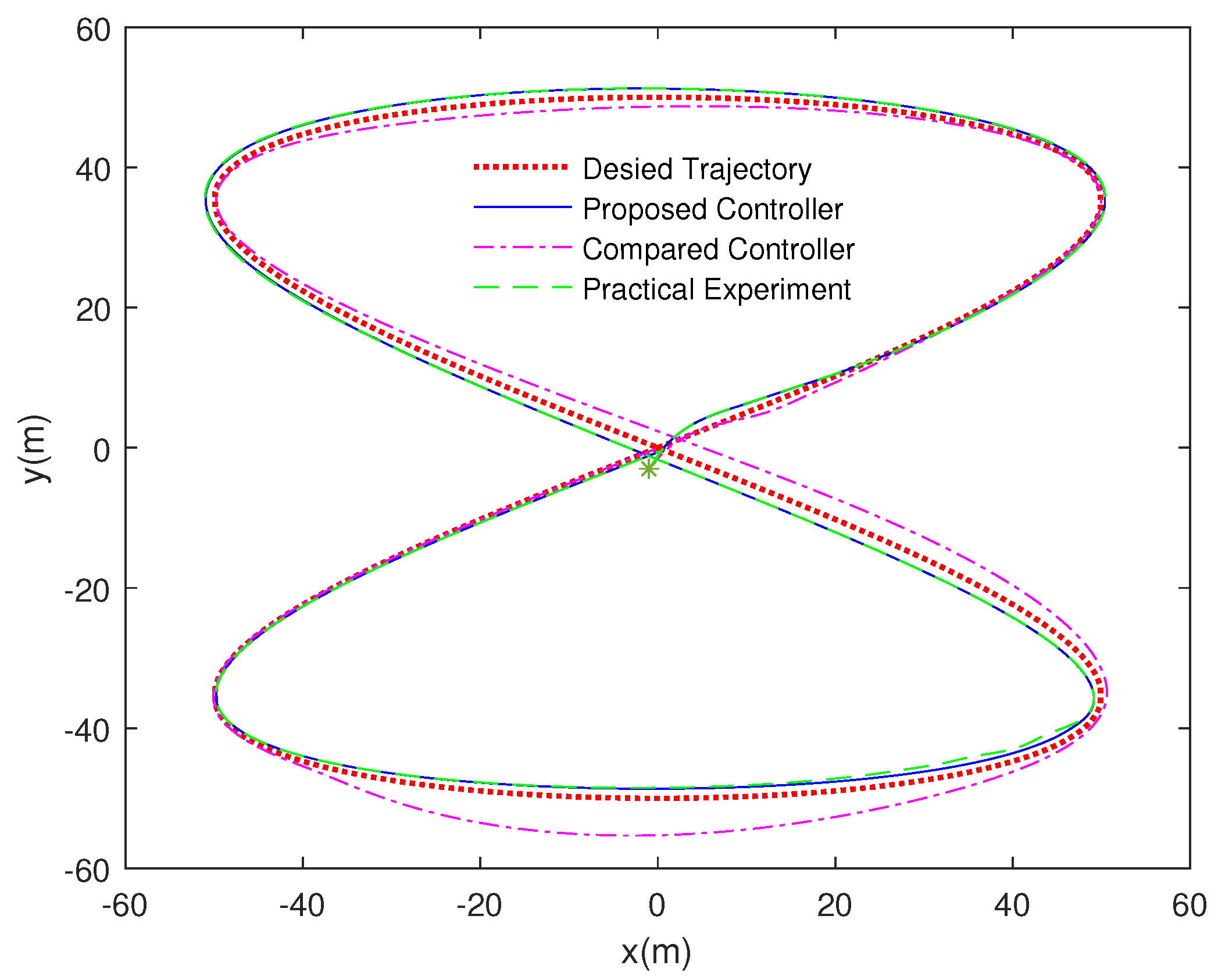
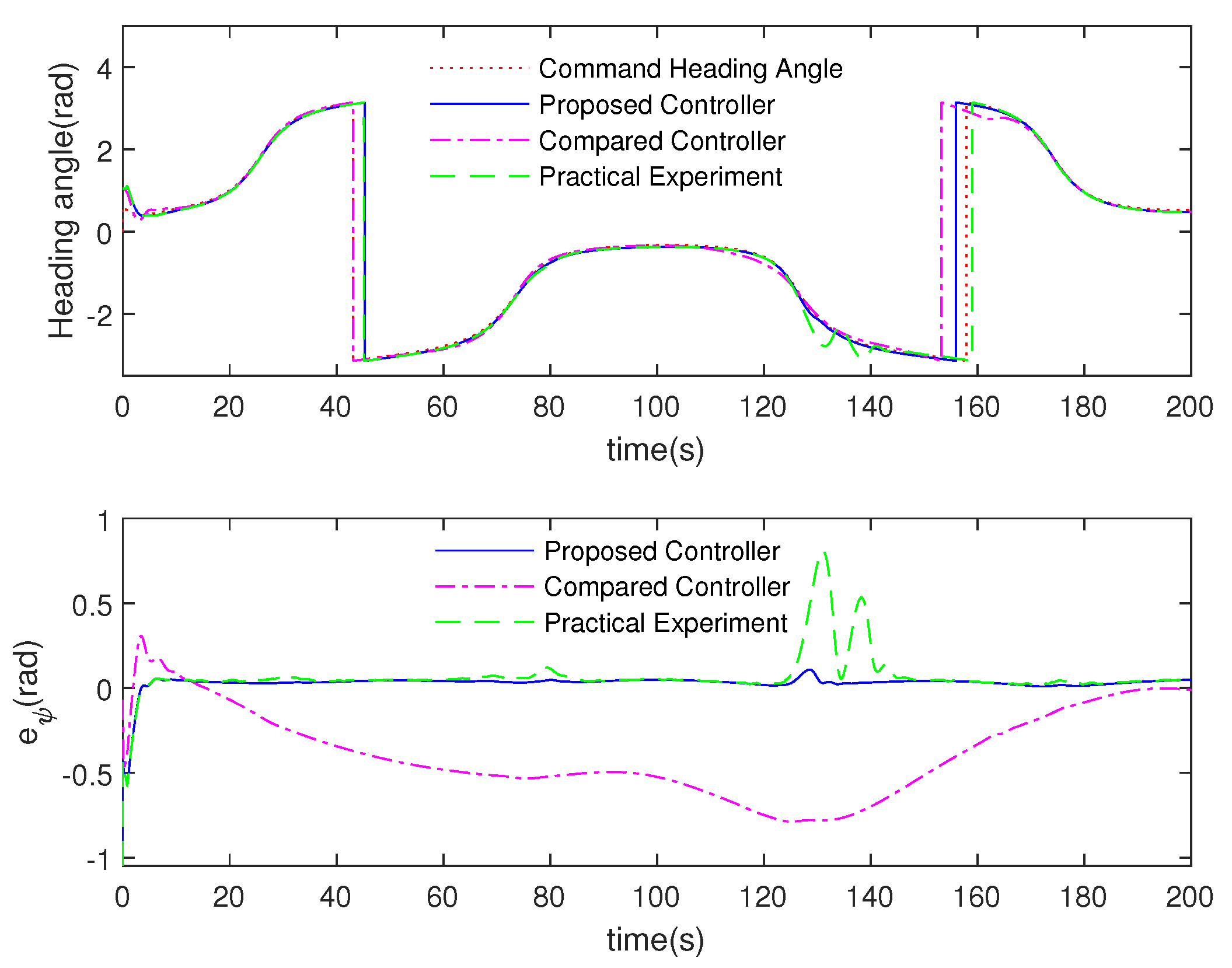
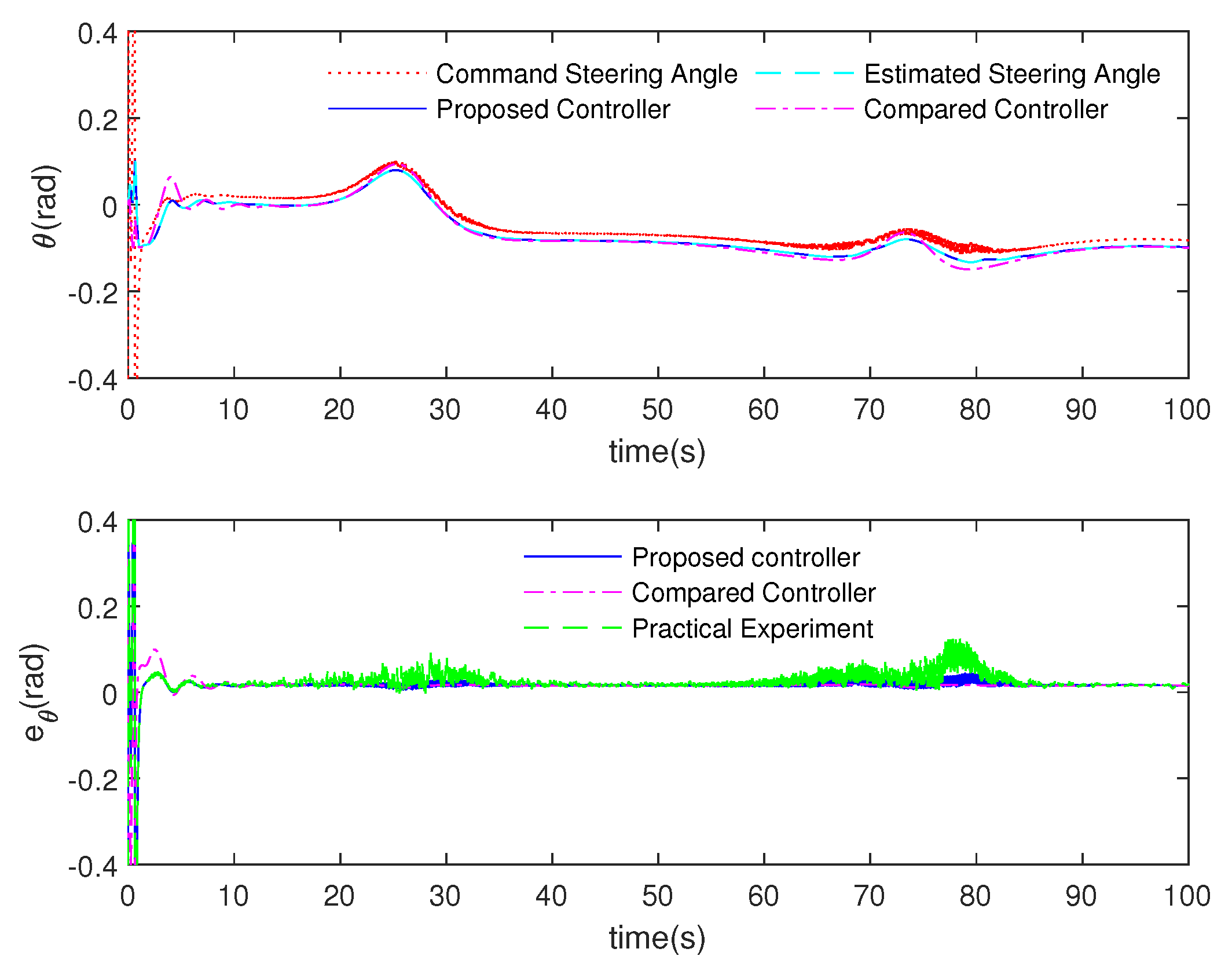
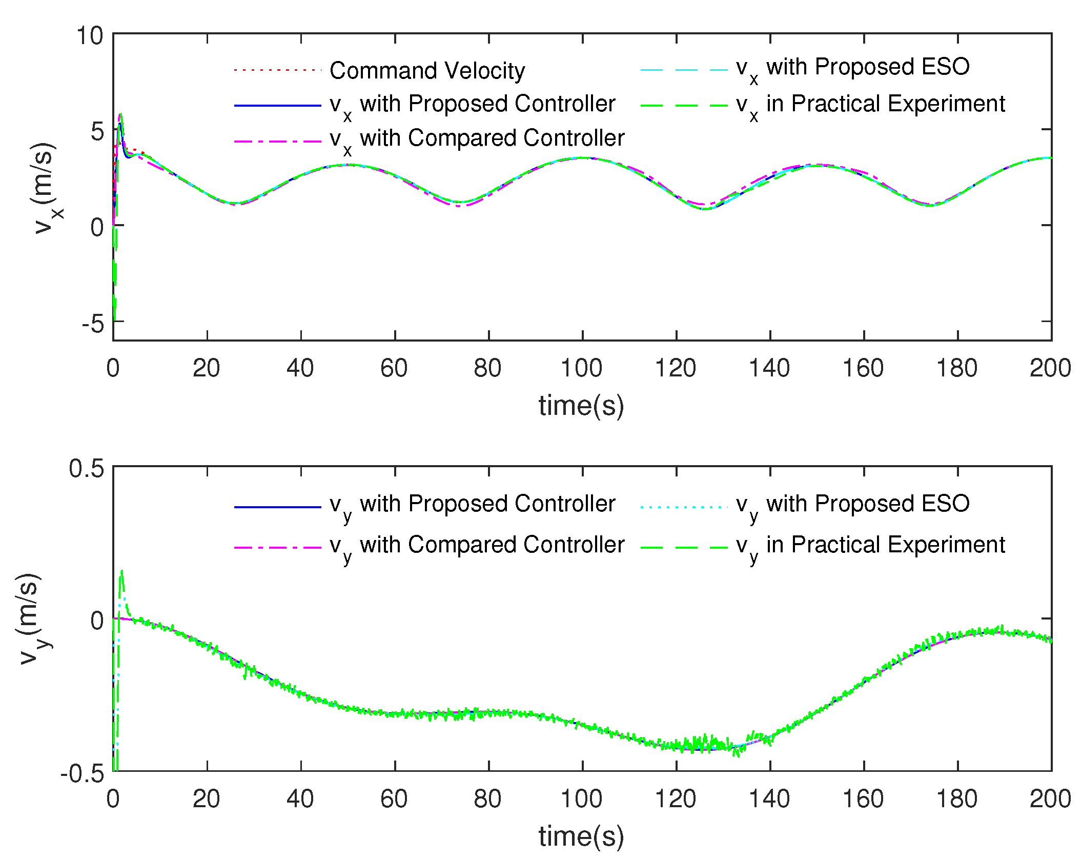
5. Experiment and Simulation Results

Experiment and simulation results are provided to illustrate the performance of the proposed controller in this section. The CLMR for the experiment is shown in Figure 3 and controller parameters, decided by the theoretic analysis in Section 4 and multiple attempts, are given as

Table 1. CLMR and controller parameters.

Parameter	Symbol & Value
CLMR mass	$m=30$
Inertia moment	$J_w=5$
Wheelbase	$L=1.2$
Kinematic controller	$k_{ax}=k_{ay}=0.6$, $k_{bx}=k_{by}=0.8$
ET-ESO for velocity	$\epsilon =0.4,q=0.8$
ESO for steering	${\beta }_1^{\theta }=30$, ${\beta }_2^{\theta }=300$, ${\beta }_3^{\theta }=1000$
Velocity controller	$k_v=0.6$, ${\xi }_v=1$
Heading controller	$k_{\psi }=1.2$, $k_{\theta }=0.5$, ${\xi }_{\theta }=0.1$, $k_{\omega }=0.65$, ${\xi }_{\omega }=0.1$

.

In order to verify the effectiveness of the proposed controller, simulation experiments without slipping compensation and practical experiment are also carried out for comparison.

The external disturbances in simulation are given by the following:

$$\left\{\begin{array}{c}{g}_{vx}\left(t\right)=-0.3+0.005\ast cos(0.05\ast t)\ast sin(0.02\ast t),\hfill \\ g_{vy}\left(t\right)=-0.01\ast sin(0.05\ast t)\ast cos(0.02\ast t),\hfill \\ g_{\omega }\left(t\right)=-0.1+0.005\ast cos(0.2\ast t)\ast sin\left(\psi \right).\hfill \end{array}\right.$$

(57)

A differential global positioning system (DGPS) module is utilized to obtain the position-heading information with 5 Hz sampling rate and a precision of $\pm 1$ cm in the practical experiment. The information is exchanged to the controller, which is realized on a platform with STM32F429, through a RS232 interface. The control period is set as 0.01 s in order to be consistent with the simulation. The experiment is carried out on the grass with uneven ground and slopes at different angles. The coordinate center is selected on the location [36${}^{\circ }$32${}^{\prime }$9${}^{″}$ N, 116${}^{\circ }$47${}^{\prime }$14${}^{″}$ E], and the same trajectory is selected as that in the simulation.

Experimental results of the aforementioned controllers are illustrated in Figure 4, Figure 5, Figure 6, Figure 7 and Figure 8. Specifically, Figure 4 shows the trajectory of CLMR, which is guided to track a preset parameterized path. It can be observed that the tracking control is achieved, regardless of skidding and slipping as well as unmeasured velocity information. Better tracking performance is achieved with the proposed controller. The tracking error in the practical experiment is appreciably increased because of the fact that the position information is not compensated when traveling on the sloping terrain.

Figure 5 depicts the heading angle and heading error. The performance of the proposed controller is obviously better, which means a smaller yaw amplitude. Figure 6 shows the steering angle. Figure 7 shows the longitudinal and lateral velocities, illustrating that the proposed ESO can recover the velocities and estimate the unknown disturbances effectively. Figure 8 depicts the control inputs for velocity and steering, and both the control inputs are bounded. The performance seems almost similar to that in Figure 5, Figure 6, Figure 7 and Figure 8; another major advantage of the proposed controller is the communication times, listed in

Table 2. Trigger times and percentage for communication.

Parameter	Event-Triggered	Time-Triggered	Percentage
Compared controller	20,000	20,000	100%
$q=0.5$	5940	20,000	29.7%
$q=0.9$	3233	20,000	16.17%

. One finds that communication times are variously reduced by using the event-triggered controller, and varies depending on different parameter settings.

It is worth noting that, compared with the time-triggered method, the performance of the control input is made worse by the ET-ESO. Less communication time is needed with a bigger q. Therefore, the balance between performance and the communication resource should be satisfied via the selection of threshold q.

6. Conclusions

In this paper, an output-based tracking controller is developed for a class of CLMR subject to slipping and skidding. An ESO is utilized to recover the velocities as well as to estimate the uncertainties and disturbances, including slipping and skidding. Constrained longitudinal velocity is established, conforming to the traffic flow theory on the kinematic level. The velocity control law and heading angle control law are developed on the dynamic level, respectively. Theoretical analysis has shown that the closed-loop system is ISS and all the signals in the closed-loop system are bounded. Finally, the simulation results are utilized to illustrate the effectiveness of the proposed controller for CLMR.

References

1. Lenain, R.; Thuilot, B.; Cariou, C.; Martinet, P. Adaptive and predictive non linear control for sliding vehicle guidance: Application to trajectory tracking of farm vehicles relying on a single RTK GPS. In Proceedings of the 2004 IEEE/RSJ International Conference on Intelligent Robots and Systems (IROS), Sendai, Japan, 28 September–2 October 2004; IEEE: Sendai, Japan, 2004; pp. 455–460. [Google Scholar]
2. Aliyu, A.; Kolo, J.G.; Mikail, O.O.; Agajo, J.; Umar, B.; Aguagba, O.I. An ultrasonic sensor distance induced automatic braking automobile collision avoidance system. In Proceedings of the 2017 IEEE 3rd International Conference on Electro-Technology for National Development (NIGERCON), Owerri, Nigeria, 7–10 November 2017; IEEE: Owerri, Nigeria, 2017; pp. 570–576. [Google Scholar]
3. Wang, L.; Liu, M. Path tracking control for autonomous harvesting robots based on improved double arc path planning algorithm. J. Intell. Robot. Syst. 2020, 100, 899–909. [Google Scholar] [CrossRef]
4. Amer, N.H.; Zamzuri, H.; Hudha, K.; Kadir, Z.A. Modelling and control strategies in path tracking control for autonomous ground vehicles: A review of state of the art and challenges. J. Intell. Robot. Syst. 2017, 86, 225–254. [Google Scholar] [CrossRef]
5. Zhu, S.; Aksun-Guvenc, B. Trajectory planning of autonomous vehicles based on parameterized control optimization in dynamic on-road environments. J. Intell. Robot. Syst. 2020, 100, 1055–1067. [Google Scholar] [CrossRef]
6. Premachandra, C.; Gohara, R.; Ninomiya, T.; Kato, K. Smooth Automatic Stopping for Ultra-Compact Vehicles. IEEE Trans. Intell. Veh. 2019, 4, 561–568. [Google Scholar] [CrossRef]
7. Low, C.B.; Wang, D. GPS-based path following control for a car-like wheeled mobile robot with skidding and slipping. IEEE Trans. Control Syst. Technol. 2008, 16, 340–347. [Google Scholar]
8. Low, C.B.; Wang, D. GPS-based tracking control for a car-like wheeled mobile robot with skidding and slipping. IEEE/ASME Trans. Mechatron. 2008, 13, 480–484. [Google Scholar]
9. Kumar, U.; Sukavanam, N. Backstepping based trajectory tracking control of a four wheeled mobile robot. Int. J. Adv. Robot. Syst. 2008, 5, 403–410. [Google Scholar] [CrossRef]
10. Wang, C.; Wang, D.; Peng, Z. Coordinated formation control of car-like mobile robots guided by parameterized single path. Control Theory Appl. 2021, 38, 1124–1132. [Google Scholar]
11. Gu, D.; Hu, H. Neural predictive control for a car-like mobile robot. Robot. Auton. Syst. 2002, 39, 73–86. [Google Scholar] [CrossRef]
12. Li, Z.; Yuan, W.; Chen, Y.; Ke, F.; Chu, X.; Chen, C.L.P. Neural-dynamic optimization-based model predictive control for tracking and formation of nonholonomic multirobot systems. IEEE Trans. Neural Netw. Learn. Syst. 2018, 29, 6113–6122. [Google Scholar] [CrossRef] [PubMed]
13. Hwang, C.; Chang, L.; Yu, Y. Network-based fuzzy decentralized sliding-mode control for car-like mobile robots. IEEE Trans. Ind. Electron. 2007, 54, 574–585. [Google Scholar] [CrossRef]
14. Hwang, C. Comparison of path tracking control of a car-like mobile robot with and without motor dynamics. IEEE/ASME Trans. Mechatron. 2016, 21, 1801–1811. [Google Scholar] [CrossRef]
15. Chen, C.; Gao, H.; Ding, L.; Li, W.; Yu, H.; Deng, Z. Trajectory tracking control of WMRs with lateral and longitudinal slippage based on active disturbance rejection control. Robot. Auton. Syst. 2018, 107, 236–245. [Google Scholar] [CrossRef]
16. Chen, M. Disturbance attenuation tracking control for wheeled mobile robots with skidding and slipping. IEEE Trans. Ind. Electron. 2017, 64, 3359–3368. [Google Scholar] [CrossRef]
17. Li, S.; Ding, L.; Gao, H.; Chen, C.; Liu, Z.; Deng, Z. Adaptive neural network tracking control-based reinforcement learning for wheeled mobile robots with skidding and slipping. Neurocomputing 2018, 283, 20–30. [Google Scholar] [CrossRef]
18. Kang, H.; Kim, Y.; Hyun, C.; Park, M. Generalized extended state observer approach to robust tracking control for wheeled mobile robot with skidding and slipping. Int. J. Adv. Robot. Syst. 2013, 10, 1–10. [Google Scholar] [CrossRef]
19. Peng, Z.; Liu, L.; Wang, J. Output-feedback flocking control of multiple autonomous surface vehicles based on data-driven adaptive extended state observers. IEEE Trans. Cybern. 2020, 51, 4611–4622. [Google Scholar] [CrossRef]
20. Peng, Z.; Wang, D.; Li, T.; Han, M. Output-feedback cooperative formation maneuvering of autonomous surface vehicles with connectivity preservation and collision avoidance. IEEE Trans. Cybern. 2020, 50, 2527–2535. [Google Scholar] [CrossRef]
21. Peng, Z.; Wang, J. Output-feedback path-following control of autonomous underwater vehicles based on an extended state observer and projection neural networks. IEEE Trans. Syst. Man Cybern.-Syst. 2018, 48, 535–544. [Google Scholar] [CrossRef]
22. Gu, N.; Peng, Z.; Wang, D.; Shi, Y.; Wang, T. Antidisturbance Coordinated Path-following Control of Robotic Autonomous Surface Vehicles:Theory and Experiment. IEEE/ASME Trans. Mechatron. 2019, 24, 2386–2396. [Google Scholar]
23. Gu, N.; Wang, D.; Peng, Z. Observer-based finite-time control for distributed path maneuvering of underactuated unmanned surface vehicles with collision avoidance and connectivity maintenance. IEEE Trans. Syst. Man Cybern.-Syst. 2020, 51, 5105–5115. [Google Scholar] [CrossRef]
24. Peng, Z.; Wang, J.; Wang, D.; Han, Q.-L. An overview of recent advances in coordinated control of multiple autonomous surface vehicles. IEEE Trans. Ind. Inform. 2021, 17, 732–745. [Google Scholar] [CrossRef]
25. Peng, Z.; Wang, J.; Wang, J. Constrained control of autonomous underwater vehicles based on command optimization and disturbance estimation. IEEE Trans. Ind. Electron. 2018, 66, 3627–3635. [Google Scholar] [CrossRef]
26. Peng, Z.; Wang, J.; Han, Q.-L. Path-Following Control of Autonomous Underwater Vehicles Subject to Velocity and Input Constraints via Neurodynamic Optimization. IEEE Trans. Ind. Electron. 2019, 66, 8724–8732. [Google Scholar] [CrossRef]
27. Peng, Z.; Jiang, Y.; Wang, J. Event-triggered dynamic surface control of an under-actuated autonomous surface vehicle for target enclosing. IEEE Trans. Ind. Electron. 2020, 68, 3402–3412. [Google Scholar] [CrossRef]
28. Peng, Z.; Wang, D.; Wang, J. Data-driven Adaptive Disturbance Observers for Model-free Trajectory Tracking Control of Maritime Autonomous Surface Ships. IEEE Trans. Neural Netw. Learn. Syst. 2021, 1–11. [Google Scholar] [CrossRef]
29. Liu, L.; Wang, D.; Peng, Z. State recovery and disturbance estimation of unmanned surface vehicles based on nonlinear extended state observers. Ocean Eng. 2019, 171, 625–632. [Google Scholar] [CrossRef]
30. Liu, L.; Zhang, W.; Wang, D.; Peng, Z. Event-triggered extended state observers design for dynamic positioning vessels subject to unknown sea loads. Ocean Eng. 2020, 209, 1–9. [Google Scholar] [CrossRef]
31. Ailon, A. Simple Tracking controllers for autonomous VTOL aircraft with bounded inputs. IEEE Trans. Autom. Control 2010, 55, 737–743. [Google Scholar] [CrossRef]
32. Khalil, H.K. Nonlinear Control; Pearson: Boston, MA, USA, 2015. [Google Scholar]
33. Khalil, H.K. Cascade high-gain observers in output feedback control. Automatica 2017, 80, 110–118. [Google Scholar] [CrossRef] [Green Version]
Figure 1. Reference frames.
Electronics 10 02886 g001
Figure 2. Scheme diagram of the controller.
Electronics 10 02886 g002
Figure 3. The CLMR and scene in practical experiment.
Electronics 10 02886 g003
Figure 4. Trajectory of the CLMR.
Electronics 10 02886 g004
Figure 5. Heading angle.
Electronics 10 02886 g005
Figure 6. Steering angle.
Electronics 10 02886 g006
Figure 7. Velocities in tracking control.
Electronics 10 02886 g007
Figure 8. Control inputs.
Electronics 10 02886 g008