Localization of Multi-Class On-Road and Aerial Targets Using mmWave FMCW Radar

Abstract

mmWave radars play a vital role in autonomous systems, such as unmanned aerial vehicles (UAVs), unmanned surface vehicles (USVs), ground station control and monitoring systems. The challenging task when using mmWave radars is to estimate the accurate angle of arrival (AoA) of the targets, due to the limited number of receivers. In this paper, we present a novel AoA estimation technique, using mmWave FMCW radars operating in the frequency range 77–81 GHz by utilizing the mechanical rotation. Rotating the radar also increases the field of view in both azimuth and elevation. The proposed method estimates the AoA of the targets, using only a single transmitter and receiver. The measurements are carried out in a variety of practical scenarios including pedestrians, a car, and an UAV, also known as a drone. With measured data, range-angle maps are created, and morphological operators are used to estimate the AoA of the targets. We also process radar range-angle images for improved visual representation. The proposed method will be extremely beneficial for practical ground stations, traffic control and monitoring frameworks for both on-ground and airborne vehicles.

1. Introduction

Radars are used in several applications both in automotive and industrial sectors. Radars for automotive applications are summarized in [1]. Applications of biomedical MIMO radars are summarized in [2]. Recently, radars were explored for air-conditioning systems [3]. Radars for medical applications are summarized in [4]. Human localization and vital signs measurements are explored, using hand-held through-wall imaging radar, in [5]. The detection and ranging of human targets in cluttered environments is proposed in [6]. The indoor human localization and life activity monitoring is proposed in [7]. mmWave radars are explored in several UAV applications [8,9,10,11,12,13,14,15]. However, radars for UAV ground station monitoring and control application is still challenging, as it needs to localize and be able to track the small dynamic UAVs in a wide field of view (theoretically 360 degrees field of view). The mmWave radars offer very high resolution, due to their large bandwidth. These radars are extremely compact, small in size and have very low power consumption. The angle of arrival (AoA), range and velocity of the targets can be estimated using them in their direct field of view (FoV). Targets at distances in the range of 300–400 m [16] can be easily detected by them at an operating frequency of a couple of GHz. An object’s range and velocity, in particular, can be accurately determined. Only a single transmitter and receiver are required to estimate target range and velocity. However, the performance of the range and velocity estimation is dependent on the chirp configuration parameters. The number of receiving antennas, on the other hand, has a large impact on the accuracy and resolution of the targets’ AoA. The combination of compressive sensing and multiple input and multiple out (MIMO) was shown to improve the angular resolution [12]. The greater the number of receiving antennas, the better the performance. The concept of MIMO is utilized to form a large number of virtual Tx–Rx pairs with limited number of Tx and Rx antennas [17]. To achieve 1 degree of angular resolution, at least 115 virtual Tx–Rx pairs are required—leading to quite a large number of physical transmitters and receivers. This also increases the hardware complexity and associated signal processing chains. As a result, mmWave radars use a small number of transmitting and receiving antennas to reduce cost and complexity.

The FoV can only be enhanced in one of two directions, due to transceiver antenna limitations: elevation or azimuth. Its main purpose is to increase the field of view in the azimuth direction, which is important for many applications. However, mmWave modules used in traffic management systems and installed as ground stations require a wide field of view in both the azimuth and elevation directions. A two-dimensional antenna array can help in widening FoV in both the elevation and azimuth directions. However, as the number of transceiver antennas grows, so does the complexity, computational latency, and cost.

An angle delay estimation method based on extended one-dimensional pseudospectrum searching is proposed in [18] The number of targets used are only two in this study, and it is computationally rigorous. The complexity of this method necessitates additional research for more than two targets. Simulating a complex scenario cannot be made possible, as the measurements in [18] were not taken in an open environment. In [19], it is proposed to develop a two-dimensional parameter estimator that combines both the extrapolated fast Fourier transform (FFT) as well as multiple signal classification (MUSIC). This study, however, does not take into account a complex scene. In [20], the range and angle estimations are proposed, employing signal parameter estimation through rotational invariance techniques (ESPRIT). Even when the number of targets exceeds the number of receivers, the proposed algorithm works. All the proposed methods need to have at least two receivers for the estimation of AoA of targets. The angle resolution improves as the number of receiving antennas increases.

A 2D synthetic-aperture radar (SAR) imaging is employed with FMCW radars [21]. The image is reconstructed using a two-dimensional FFT or range Doppler plot. Because of the fixed horizontal and vertical movement, this approach can capture the target in a constant FoV. This limits the user’s ability to capture a variety of scenarios. However, localization of multiple targets remains challenging.

In [22], a fan-beam antenna is used to implement a three-dimensional (3D) view of mmWave radar, finding its application in mobile robotics. There is a lack of information on AoA and additionally, there are limitations regarding the measurements in range and velocity. In [23], it was proposed to use 3D near-field imaging for robotics and security scanning. In this work, they combine LiDAR data, which adds to the computational complexity and delay. In [24], a synthetic aperture mmWave ground station search and track radar is proposed. It has numerous drawbacks, such being large, complicated, and lacking target AoA calculation for rotating radars. The rotating FMCW radar is used for localization and mapping. The task is used to determine the target’s range and velocity. The majority of these works have not concentrated on multiple target localization, which is crucial for a wide range of applications. A mechanical scanning FMCW radar is proposed in [25]. It uses the bandwidth of 400 MHz only. However, detailed experiments and automatic angle estimation for multi target scenarios are still missing. A 3D millimeter wave system is proposed in [26] for robotic mapping and localization, as well as security scan applications. It mainly focuses on indoor short-range applications. Practical multi-target outdoor scenarios still need further investigation.

To address the aforementioned issues, we present a rotating mmWave FMCW radar capable of detecting the target range and AoA. We utilize range-angle maps computed from a 1D range FFT profile for localization. It is possible to obtain target features, such as distance and velocity [27,28], accurately with fixed positioning of radars, but it is difficult to accurately estimate AoA of the targets with a limited number of receiving antennas. Using our AoA estimation approach, we can locate and estimate the AoA of objects in a wide field of view. This FoV is also configurable, allowing it to be adjusted to the demands of the application. The major contributions of this paper are as follows:

• We propose AoA estimation of multi-class targets by mmWave FMCW radar measurements in a practical outdoor setting.
• The proposed method just requires only 1 Tx antenna and 1 Rx antenna for the localization of multi-class targets.
• The proposed localization method using mmWave FMCW radar achieves a large FoV in both azimuth and elevation directions.
• The proposed method estimates the AoA of both on-road and aerial targets, using morphological operators on range-angle maps.
• The proposed method improves the visual representation of multi-class targets, using range–angle images.

The paper is further organized as follows. Section 2 discusses the details of the radar system. Section 3 elaborates on the measurements and signal processing. Section 4 presents the angle of arrival estimation of multiple targets, using morphological operators on range–angle maps. Results are discussed in Section 5. Finally, in Section 6, the conclusion and potential future works are discussed.

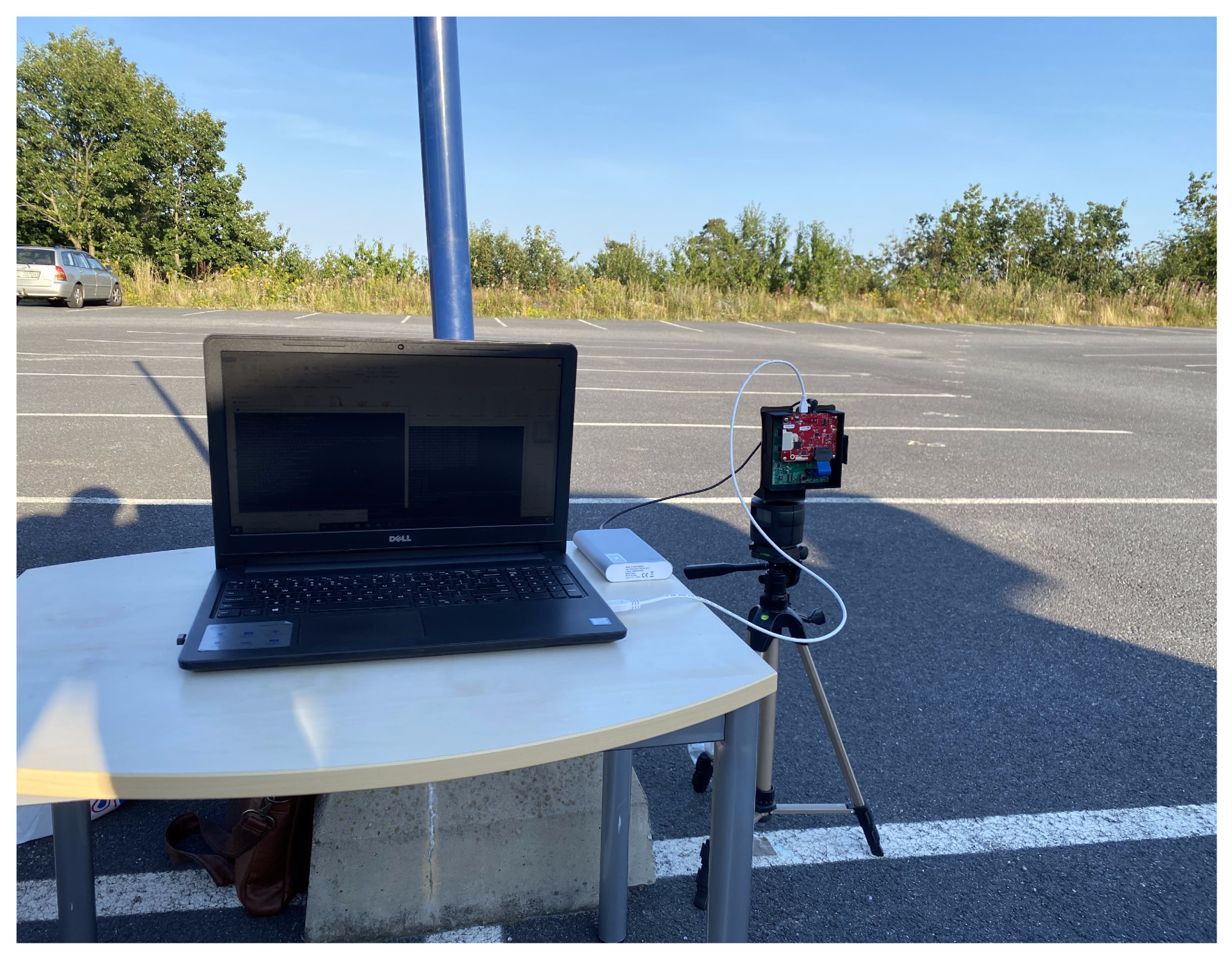
2. System Description

The measurements were taken with a Texas Instruments (TI) mmWave radar with three transmitters and four receivers [29]. The radar’s comprehensive details can be found in Figure 1. The received signal is mixed with the transmitted FMCW signal’s quadrature phase and in-phase as shown in Figure 1. The output signal is a complex intermediate frequency (IF) signal, which is subsequently converted into digital form using ADCs for further processing. The FMCW radar has an RF bandwidth of 4 GHz and works at frequencies ranging from 77 GHz to 81 GHz. The radar configurations parameters can be seen in

Table 1. Configuration parameters for mmWave radar [30].

S. No.	Parameter	Value
1	RF Frequency Range	77–81 GHz
2	Chirp Slope	29.982 MHz/μs
3	Number of Transmitters	3
4	Number of Receivers	4
5	Number of ADC samples	256
6	Number of frames	800
7	Number of Chirps	128
8	RF Bandwidth	1798.92 MHz
9	Frame periodicity	40 ms
10	Sampling Rate	10 MSPS
11	Drone Size	322 × 242 × 84 mm
12	Human Height	172 cm
13	Car Size	4315 × 1780 × 1605 mm
14	Measurement Range	up to 26 m
15	Transmission Power	12 dBm
16	Rx Noise Figure	14 dB (76 GHz to 77 GHz)
		15 dB (77 GHz to 81 GHz)

.

The complete radar system is mounted on a programmable rotor as shown in Figure 2. In each measurement case, every frame is used to capture the raw intermediate frequency (IF) data. The single frame time is set at 40 milliseconds. A frame is made up of a specific number of chirps. We chose 128 chirps per frame. The raw radar data from the measurements are then post-processed in MATLAB [31]. The measurements are carried out by positioning the multiple targets, such as an aerial vehicle/drone, humans, and an automobile car, at various distances and angles. Each measurement scene is referred to as a separate instance in which the positions of the individuals, automobile car, and drone are all jumbled together. The complete details of various measurement scenes are summarized in

Table 2. Measurement cases (range in meters and angle in degrees).

	Cases	a	b	c	d	e	f	g	h	i	j	k	l	m	n
Targets
Human-1	Range	9	13	11	13	7	17	5	19	5	9	21	7	15	7
	Angle	30	60	0	0	60	30	60	90	90	120	180	120	180	30
Human-2	Range	11	15	13	15	9	19	7	11	7	21	23	5	7	17
	Angle	60	90	30	30	90	60	90	120	120	60	0	180	0	0
Human-3	Range	13	17	17	17	13	21	11	9	13	7	5	11	11	9
	Angle	90	120	90	60	150	90	150	150	180	180	150	60	30	60
Human-4	Range	15	19	19	21	15	23	21	7	15	23	13	15	13	11
	Angle	120	150	120	120	0	120	0	0	60	90	90	90	120	120
Human-5	Range	17	11	21	23	19	9	23	25	17		17	19	17	13
	Angle	150	180	150	150	30	0	30	60	0		30	150	150	150
Drone	Range	5	7	9	11	5	7	9	5	11	5	7	9	9	5
	Angle	0	30	60	90	120	150	180	30	30	150	60	30	90	90
	Cases	aa	bb	cc	dd	ee	ff	gg	hh	ii	jj	kk	ll	mm	nn	oo
Targets
Drone	Range	7	9	11	5	9	11	7	7	9	11	9	11	5	7	11
	Angle	0	0	0	60	60	60	90	120	120	120	150	150	180	180	180
Car	Range	25	19	17	15	17	17	21	23	15	21	17	23	15	21	25
	Angle	60	60	90	120	150	180	180	90	0	0	0	90	60	120	30

.

The radar transmitted signal is given by Equation (1):

$$\begin{array}{cc}\hfill T\left(t\right)& =sin[j{\varphi }_i+j2\pi (\frac{\beta }{2}{t}^2+f_{s}t)],0\le t\le T_c\hfill \end{array}$$

(1)

In Equation (1), $f_s$ is the chirp’s starting frequency, ${\varphi }_i$ is the initial phase of the chirp, $\beta$ is the slope of the chirp, and $\beta$ is given by the following:

$$\begin{array}{c}\hfill \beta =\frac{f_f-f_s}{T_c}\end{array}$$

(2)

$f_f$ is the chirp’s final frequency, and $T_c$ is the chirp time over which the chirp’s frequency changes from $f_s$ to $f_f$. The transmitted chirp’s frequency is given by Equation (3):

$${\omega }_T\left(t\right)=2\pi (\frac{\beta }{2}t+f_s)$$

(3)

The received signal, R(t) reflected off the distant targets, is a delayed version of the transmitted signal, T(t). R(t) is denoted by the following:

$$R\left(t\right)=T(t-\tau )$$

(4)

The round trip time delay, $\tau$ is defined by the following:

$$\tau =2R/c$$

(5)

where R denotes the distance of the detected target from radar, and c denotes the speed of light. The reflected signals from distant targets are mixed with the transmitted signal’s in-phase and quadrature phase, and the complex IF signal is generated as shown in Figure 1. This IF signal is processed further and digitized, using ADCs at a sampling frequency of 10 MSPS [32]. This IF signal’s frequency is proportional to the range of the target in direct line of sight (D-LOS) that reflects the transmitted chirp by Equation (6).

$$f_{IF}=\frac{(f_f-f_s)·2R}{T_c·c}$$

(6)

$$R=\frac{f_{IF}·c}{2\beta }$$

(7)

where R, $f_{IF}$, and c are the range, intermediate frequency, and velocity of light in vacuum, respectively.

Range profiles are computed from the measured raw data and further processed to obtain the range–angle maps [30].

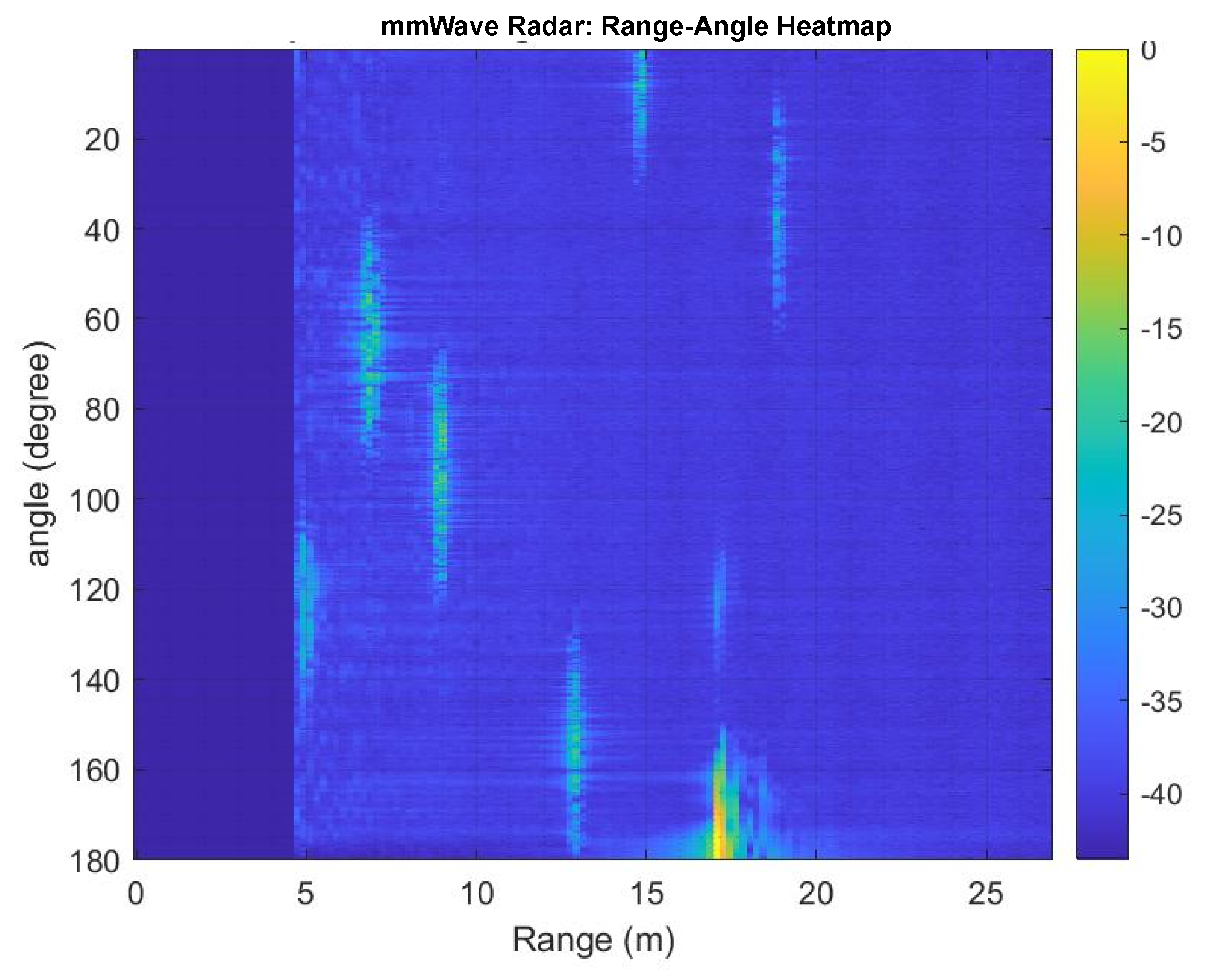
3. Outdoor Measurements and Pre-Processing

The measurements are taken in a realistic outdoor setting with a multiple targets in the scene. The raw radar data are used for the creation of range–angle maps of all measurement scenes. These range–angle maps are further processed using morphological operators. Several measurement scenes were captured; the summary of all the measurement instances can be found in Table 2. For instance, in case-a, human-1 is positioned at 30${}^{\circ }$ and 9 m distance, human-2 is positioned at 60${}^{\circ }$ and 11 m distance, human-3 is positioned at 90${}^{\circ }$ and 13 m distance, human-4 is positioned at 120${}^{\circ }$ and 15 m distance, and human-5 is positioned at 150${}^{\circ }$ and 17 m distance from the radar. Additionally, a drone is positioned at 0${}^{\circ }$ and 5 m distance, and a car is positioned at 0${}^{\circ }$ and 19 m distance. During all measurements, the raw IF data are captured from the mmWave radar. The raw radar data are then processed using MATLAB, and the details can be accessed at [33]. Range–angle heatmaps are created for all measurement scenes [30]. The generation of the angle axis for the range–angle maps is briefly described here.

A programmable rotor is attached to a radar to cover certain FoV, ${\theta }_{FoV}$, in T seconds. The radar transmits $N_f$ frames to cover the same FoV, ${\theta }_{FoV}$ in T seconds. Thus, this entire ${\theta }_{FoV}$ is divided into angle bins, denoted by ${\theta }_{bin}$.

The angle bins (${\theta }_{bin}$), total FoV (${\theta }_{FoV}$), and total number of frames ($N_f$) are related by Equation (8):

$$\begin{array}{c}\hfill {\theta }_{bin}=\frac{{\theta }_{FoV}}{N_f}\end{array}$$

(8)

In the outdoor measurements, we set ${\theta }_{FoV}$ to ${180}^{\circ }$ and $N_f$ is set to 800, then each frame corresponds to 0.225${}^{\circ }$, i.e., 4.44 frames per degree. A range–angle heat map is then plotted using the range profiles. Such range–angle heat maps for the measurement of case-e and measurement of case-f can be seen in Figure 3 and Figure 4, respectively.

4. Range and Angle Estimation Using Morphological Operators on Range–Angle Maps

Image processing techniques were used to process the range–angle map images after obtaining them. The flowchart in Figure 5 depicts the various processing steps.

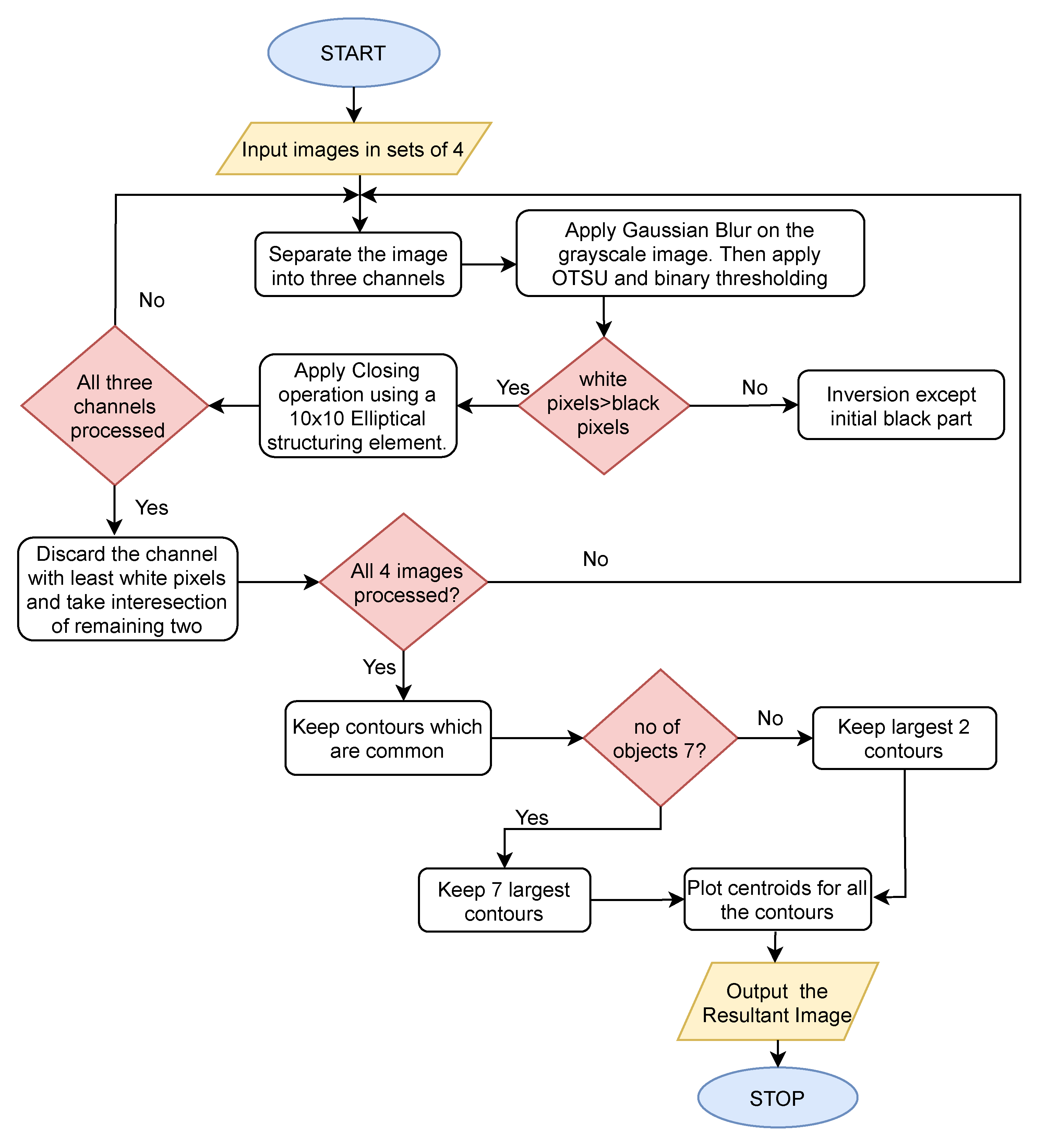
• Because four receivers were used here, the data set was divided into four sets, one for each case, and four different receivers capturing it. The images were then processed one by one. However, only 1 Tx and 1 Rx are required for angle estimation using the proposed method.
• The image was cropped off the scale using Otsu thresholding, and objects were displayed based on the most definite contour, which is the largest in area.
• An image was then divided into three channels, namely BGR, stored in a list, and converted into gray scale images. Individual channels were then processed.
• To smooth out the image, Gaussian blurring was used, followed by Otsu thresholding, to remove noise and binarize it.
• After obtaining the binary image, inversion based on the number of white and black pixels was performed, followed by the morphological operation, closing with a 10 × 10 elliptical structuring element to obtain proper contours. Any areas with a size smaller than 150 px*px were removed.
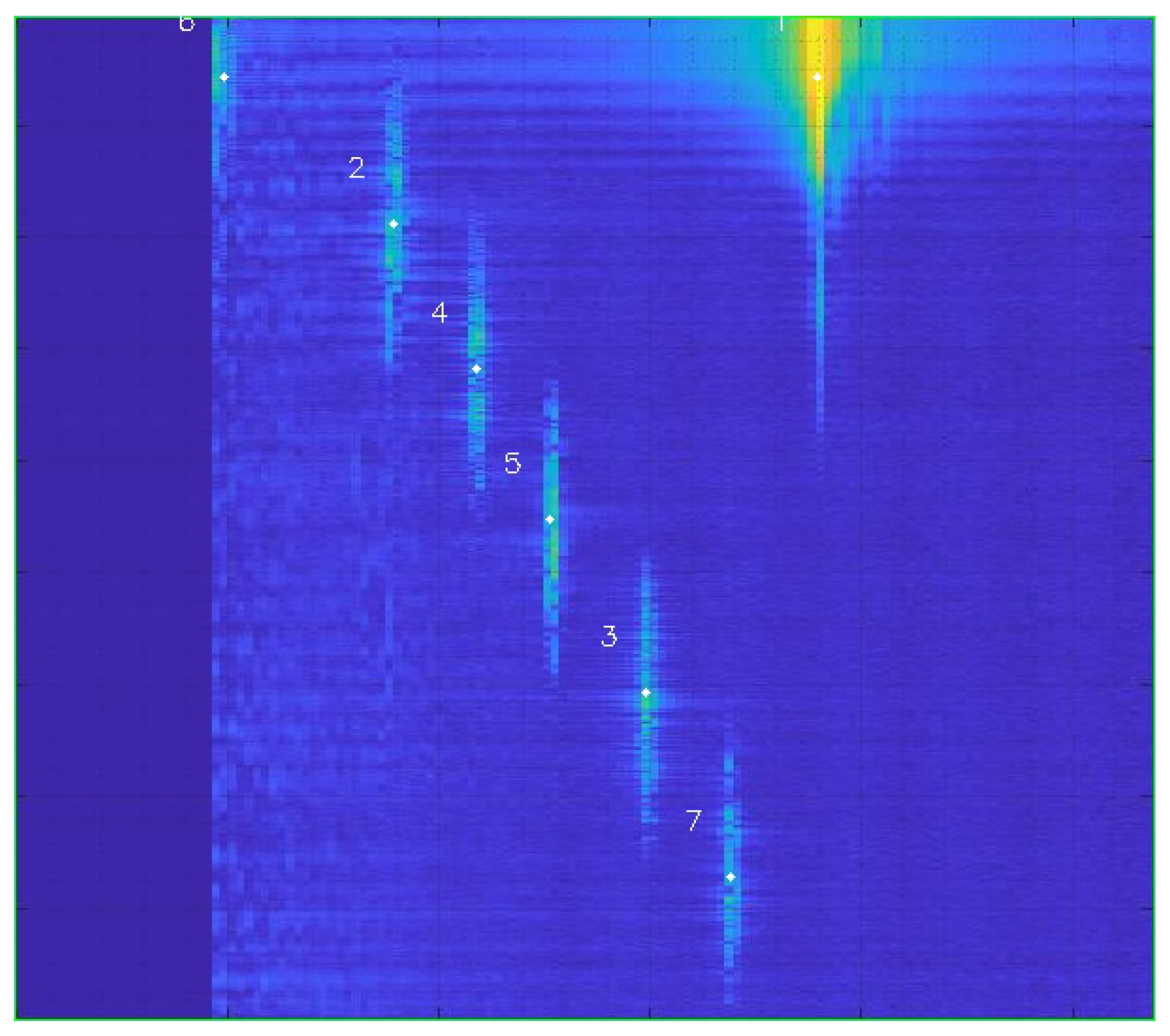
• The best two of the three channels were then chosen, and their intersection was used to generate the final processed image. Later, only contours with a common area in at least three of the four images were kept, and the best contours based on the number of objects were chosen.
• Finally, using the concept of moments, the centroids were plotted.

4.1. Otsu Thresholding

Image segmentation employs the use of thresholding. It is used to turn a grayscale image into a binary image. Its algorithm operates in such a way that it replaces each pixel if its intensity is less than a fixed constant T threshold value. This value is determined in Otsu thresholding so that the weighted within-class variance can be obtained [34]. The relation is as follows:

$$\begin{array}{c}\hfill {\sigma }_w^2\left(t\right)=q_1\left(t\right){\sigma }_1^2\left(t\right)+q_2\left(t\right){\sigma }_2^2\left(t\right)\end{array}$$

(9)

where

$$\begin{array}{c}\hfill q_1\left(t\right)=\sum _{i=1}^{t}P\left(i\right)\&q_2\left(t\right)=\sum _{i=t+1}^{I}P\left(i\right)\end{array}$$

(10)

$$\begin{array}{c}\hfill {\mu }_1\left(t\right)=\sum _{i=1}^t\frac{iP\left(i\right)}{q_1\left(t\right)}\&{\mu }_2\left(t\right)=\sum _{i=t+1}^I\frac{iP\left(i\right)}{q_2\left(t\right)}\end{array}$$

(11)

$$\begin{array}{c}\hfill {\sigma }_1^2\left(t\right)=\sum _{i=1}^t{\left[i-{\mu }_1\left(t\right)\right]}^2\frac{P\left(i\right)}{q_1\left(t\right)}\&\end{array}$$

(12)

$$\begin{array}{c}\hfill {\sigma }_2^2\left(t\right)=\sum _{i=t+1}^I{\left[i-{\mu }_2\left(t\right)\right]}^2\frac{P\left(i\right)}{q_2\left(t\right)}\end{array}$$

(13)

Unlike global thresholding, which selects any arbitrary value as a threshold value, Otsu thresholding involves looping through all possible threshold values and fixing the value whose value is the minimum by calculating the spread through the above formulae on both the foreground and background sides of pixels [34].

In this case, Otsu thresholding is used to remove the scaling from the original image so that processing can take place. Later, Otsu is used to convert the grayscale image to a binary image because the morphological operation can be performed on a binary image with only two pixel intensities to deal with. The resulting image can be seen in Figure 6.

4.2. Gaussian Blurring

The pixels closest to the center are given the most weightage in Gaussian blurring. A group of pixels, referred to as a kernel, is slid along the pixel that needs to be filtered. The weighted average of pixel intensities is calculated to apply this filter [35]. The Gaussian blur filter is simply convolving the image with a Gaussian function, as shown below:

$$\begin{array}{c}\hfill G(x,y)=\frac{1}{2\pi {\sigma }^2}{e}^{-\frac{x^2+y^2}{2{\sigma }^2}}\end{array}$$

(14)

Here, x is the horizontal distance from the origin, y is the vertical distance from the origin, and $\sigma$ is the Gaussian distribution’s standard deviation. The values of these Gaussian functions combine to form a convolution matrix, which is then used to convolve the original image [36]. The weighted mean of each pixel’s neighbor is then used to replace it. After obtaining three channel images as shown in Figure 7, Gaussian blurring is used to remove noise. Then, the filtered image is thresholded and converted into a binary image.

4.3. Morphological Operation-Closing

Closing is a morphological operator derived from erosion and dilation [37]. It is typically used on binary images. It enlarges the boundaries of images’ bright parts and fills gaps in such areas. It is dilation followed by erosion, and it keeps the areas that have a similar shape to the structuring element, while removing the other pixels [37].

Dilation fills holes in images, which can lead to pixel distortion; erosion reduces this. Finally, a structuring element is taken and moved across the image (outside the foreground region). If the SE touches the point and is not part of the foreground region, then that region becomes the background; otherwise, it becomes the foreground [37]. Closing can be mathematically represented as follows:

$$\begin{array}{c}\hfill A•B=(A\oplus B)\ominus B\end{array}$$

(15)

Following the application of the closing operation, other bounds are applied to the image, such as classification and selection based on the contour area (the minimum bound is selected as 150 px*px based on observation), and then the best channel and contour intersection as explained in the algorithm. Finally, long horizontal lines with a width bound of 46 are removed, and the resultant processed image is shown in Figure 8.

4.4. Concept of Moments

Moments of a function are quantitative characteristics of a function’s shape in mathematics [38]. In this case, we used the zeroth moment to represent mass, which when divided by the total mass yields the center of mass. Contours are laminas, and their geometric center is a centroid; because we assumed that the density of a lamina is constant [39], their center of mass and centroid coincide. Following that, in order to obtain proper contours (laminae), we drew a parallel between the intensity of pixels and the mass of an object, and then divided by the total mass to obtain the center of mass, which is the centroid of the lamina or contour. We employed the bounding rectangle concept [39] because we assumed the lamina to be a rectangle such that the contour is completely enclosed and touches the boundaries of the rectangle. Its centroid is calculated using the formulae given below. Moments are calculated as follows:

$$\begin{array}{c}\hfill {\mathrm{m}}_{\mathrm{ji}}=\sum _{\mathrm{x},\mathrm{y}}\left(array(\mathrm{x},\mathrm{y})·{\mathrm{x}}^{\mathrm{j}}·{\mathrm{y}}^{\mathrm{i}}\right)\end{array}$$

(16)

The COM or the centroid in this case is computed as follows:

$$\begin{array}{c}\hfill \overline{x}=\frac{m_{10}}{m_{00}},\overline{y}=\frac{m_{01}}{m_{00}}\end{array}$$

(17)

Here, $\overline{x}$ and $\overline{y}$ represent the center of mass of the x coordinate and y coordinate of the contour, respectively. The centroid of each object in the image is shown in Figure 9.

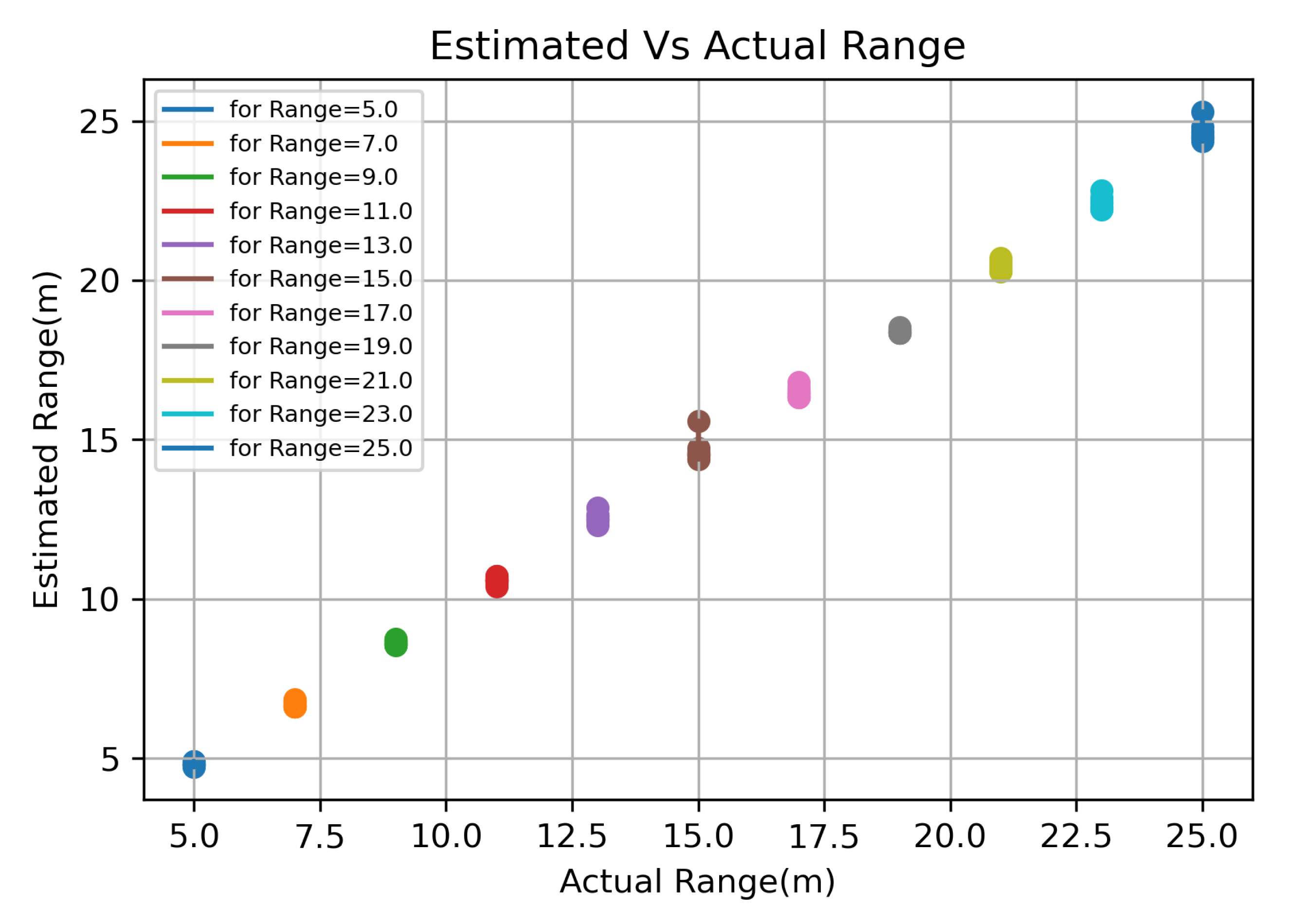
5. Results and Discussion

Using all image processing techniques, including Gaussian blurring, Otsu thresholding, inversion, closing, and center of moments, we calculated the centroid of each contour, which represents the location of an object. The centroid’s (x, y) coordinates represent (range, angle). Graphs were formulated to show the spread of values across a specific range/angle. How close the actual and estimated values were are shown in the Bland–Atman plot.

The spread of values in range is almost negligible, as demonstrated by Figure 10 and Figure 11 which depict the spread of angle values; it is observed that the spread is high at the edges, i.e., at 0 and 180 degrees, because the radar angle should have started from a negative angle to obtain accurate values, but it was started from 0 degrees, resulting in higher variance at the extreme values of the angles. The x-axis in Figure 10 and Figure 11 represents the actual measured ranges/angles, and the y-axis represents the obtained values of ranges using the image processing techniques of radar images.

Statistical Analysis of Measurements

In the literature, two kinds of measurement accuracy evaluation techniques were used to find the closeness between the actual values and the measured values (or estimated values): (i) the Pearson correlation (PC) coefficient with linear regression parameters computed for the actual and measured values, and (ii) the Bland–Altman plot with a set of benchmark metrics, such as bias, standard deviation (SD), limit of agreement (LOA), and Bland–Altman ratio (BAR). If the PC value is close to 1, then the measured values nearly equal the actual values. If the BAR value is <10%, then the agreement between the actual and measured time series is good. The agreement is moderate if 10% < BAR ≤ 20%, and is insufficient if the BAR > 20%.

The Pearson correlation (PC) coefficient is computed as follows:

$$\mathrm{PC}=\frac{{\sum }_{i=1}^N(x_i-\overline{x})(y_i-\overline{y})}{\sqrt{{\sum }_{i=1}^N{(x_i-\overline{x})}^2{\sum }_{i=1}^N{(y_i-\overline{y})}^2}}.$$

(18)

where $\overline{x},\overline{y}$ denote the mean of actual and measured values, respectively. The bias, standard deviation (SD), limit of agreement (LOA), acceptance limit (AL), and Bland–Altman ratio (BAR) metrics are computed from the Bland–Altman plot by using following formulae [40]:

$$\mathrm{Bias}=\frac{1}{N}\sum _{i=1}^n(y_i-x_i)$$

(19)

Bias indicates a mean shift in the measured values relating to the actual values.

$$\mathrm{SD}=\sqrt{\frac{1}{N-1}\sum _{i=1}^n{(y_i-x_i-\mathrm{Bias})}^2}$$

(20)

The SD denotes the differences between the actual (x) and measured (y) values.

$$\mathrm{LOA}=\mathrm{Bias}\pm 1.96\mathrm{SD}$$

(21)

LOA indicates the agreement limits.

$$\mathrm{AL}=\pm \frac{1}{N}\sum _{i=1}^N\frac{y_i+x_i}{2}$$

(22)

$$\mathrm{BAR}=\frac{1.96\mathrm{SD}}{\frac{1}{N}{\sum }_{i=1}^N\frac{y_i+x_i}{2}}$$

(23)

The BAR parameter relates SD to the acceptance limit (AL).

From the error analysis shown in

Table 3. Results of measurement error analysis using the Pearson correlation coefficient, and the bias, SD, and BAR metrics obtained from Bland–Altman analysis ^a.

Measurement	PC	Bias	SD	LOA (Biasą1.96*SD)		AL	BAR
				Bias+1.96*SD	Bias-1.96*SD
Range	0.9996	−0.4143	0.1941	−0.0339	−0.7946	13.7595	0.0276
Angle	0.9954	3.6176	6.4824	16.3232	−9.0879	89.3088	0.1423

^a PC: Pearson Correlation Coefficient; SD: Standard Deviation; LOA: Limits of Agreement; AL: Acceptance Limit; BAR: Bland—Altman ratio.

and Figure 12, it is observed that proposed measurement method has a range bias of −0.4142 with 95% agreement limits of [−0.7945, −0.0339] m and the angle bias of 3.617 with 95% agreement limits of [−9.087, 16.32] degrees. For the same error analysis, the Pearson correlation coefficient is 99.96 for the range measurements, indicating better correlation between the measured and actual values. The proposed method has a BAR value of 2.76%, which indicates very good agreement between the measured and actual range values. It is further noticed that the method has a BAR value of 14.23% for the measurement of angles, although the Pearson correlation coefficient is 99.54; therefore, we further investigated the angle measurements for different error ranges. From the angle measurement error analysis, we noticed that the method has an angle error of <3${}^{\circ }$ for 29 targets, 3–6 for 29 targets, 6–10 for 45 targets, >10 for 17 targets. For the 18 targets with zero angle, the method has an angle error of >8${}^{\circ }$ for 17 targets. The statistical analysis results in Table 3 and Figure 12 show that the bias, LOA and BAR values of the proposed measurement method have a high degree of agreement between the actual and estimated range and angle values.

Considering the results and deviation, it is possible to conclude that the proposed image processing method, which employs morphological operator closing to obtain definite contours, is accurate on almost all ranges and angles, except the extremes. This image processing technique is lightweight and does not necessitate a large amount of computation.

The proposed model’s complexity and performance merits are compared to [20,41,42,43,44].

Table 4. Performance comparison table ^a.

S. No.	Algorithm	Complexity	Targets at Same Range/Angle	Detection Limitation of Targets	Required Number of Antennas for AoA Estimation	Reference
1.	DFT-ESPRIT	$Nlog\left(N\right)$	No	Multiple targets	1 TX and 2 RX	[41]
2.	2D-ESPRIT	$\frac{2R{n}^2{N}^3}{27}$	No	Multiple targets	1 TX and 2 RX	[42]
3.	Dual-Smoothing	$\frac{10R{n}^2{N}^3}{27}$	No	Multiple targets	1 TX and 2 RX	[43]
4.	Clustered ESPRIT	$\frac{N^3}{28}$	Yes	RX antennas could be smaller than number of targets	RX antennas could be smaller than number of targets	[20]
5.	Range-Angle	$Nlog\left(N\right)$	Yes	No limitation	1 TX and 1 RX	[44]
	map based
6.	Proposed work	$Nlog\left(N\right)$	Yes	No limitation	1 TX and 1 RX	This work

^a N: Numbero f samples, R_n: Numbero f RXantennas.

shows that the proposed model computational complexity is similar to [44] and has a large FoV in both azimuth and elevation when compared to the rest of the designs and/or algorithms that were reported. However, the work in [44] considered only human targets, whereas the proposed work considered both on-road and aerial targets simultaneously. To estimate the angle, only one Tx and one Rx antenna were required in the proposed concept. Furthermore, there is no limit to the number of targets that can be detected.

6. Conclusions

We present a novel AoA estimation technique based on mechanical rotation using mmWave FMCW radars in this paper. The proposed method estimates the AoA of multiple targets using only a single transmitter and receiver. The measurements were taken in real-world scenarios involving pedestrians, a car, and an UAV. Based on the measurements and collected radar data, range-angle maps are created, and morphological operators were used to estimate the AoA of the multiple targets. Furthermore, we demonstrated radar range–angle images for improved visual representation. The proposed method will be extremely beneficial for ground stations, traffic control and monitoring applications for both on-ground and airborne vehicles. The cross range resolution is an interesting study. However, this requires a large number of outdoor experiments. We plan to continue our work in the future by taking more outdoor measurements.

References

1. Gamba, J. Automotive Radar Applications. In Radar Signal Processing for Autonomous Driving; Springer: Singapore, 2020; pp. 123–142. [Google Scholar] [CrossRef]
2. Cardillo, E.; Caddemi, A. A Review on Biomedical MIMO Radars for Vital Sign Detection and Human Localization. Electronics 2020, 9, 1497. [Google Scholar] [CrossRef]
3. Cardillo, E.; Li, C.; Caddemi, A. Embedded heating, ventilation, and air-conditioning control systems: From traditional technologies toward radar advanced sensing. Rev. Sci. Instruments 2021, 92, 061501. [Google Scholar] [CrossRef] [PubMed]
4. Pisa, S.; Pittella, E.; Piuzzi, E. A survey of radar systems for medical applications. IEEE Aerosp. Electron. Syst. Mag. 2016, 31, 64–81. [Google Scholar] [CrossRef]
5. Yang, D.; Zhu, Z.; Zhang, J.; Liang, B. The Overview of Human Localization and Vital Sign Signal Measurement Using Handheld IR-UWB Through-Wall Radar. Sensors 2021, 21, 402. [Google Scholar] [CrossRef] [PubMed]
6. Cardillo, E.; Caddemi, A. Radar Range-Breathing Separation for the Automatic Detection of Humans in Cluttered Environments. IEEE Sens. J. 2021, 21, 14043–14050. [Google Scholar] [CrossRef]
7. Wang, G.; Gu, C.; Inoue, T.; Li, C. A Hybrid FMCW-Interferometry Radar for Indoor Precise Positioning and Versatile Life Activity Monitoring. IEEE Trans. Microw. Theory Tech. 2014, 62, 2812–2822. [Google Scholar] [CrossRef]
8. Dogru, S.; Marques, L. Pursuing Drones with Drones Using Millimeter Wave Radar. IEEE Robot. Autom. Lett. 2020, 5, 4156–4163. [Google Scholar] [CrossRef]
9. Rai, P.K.; Idsøe, H.; Yakkati, R.R.; Kumar, A.; Ali Khan, M.Z.; Yalavarthy, P.K.; Cenkeramaddi, L.R. Localization and Activity Classification of Unmanned Aerial Vehicle Using mmWave FMCW Radars. IEEE Sens. J. 2021, 21, 16043–16053. [Google Scholar] [CrossRef]
10. Morris, P.J.B.; Hari, K.V.S. Detection and Localization of Unmanned Aircraft Systems Using Millimeter-Wave Automotive Radar Sensors. IEEE Sens. Lett. 2021, 5, 1–4. [Google Scholar] [CrossRef]
11. Cidronali, A.; Passafiume, M.; Colantonio, P.; Collodi, G.; Florian, C.; Leuzzi, G.; Pirola, M.; Ramella, C.; Santarelli, A.; Traverso, P. System Level Analysis of Millimetre-wave GaN-based MIMO Radar for Detection of Micro Unmanned Aerial Vehicles. In 2019 PhotonIcs Electromagnetics Research Symposium—Spring (PIERS-Spring); Springer: Singapore, 2019; pp. 438–450. [Google Scholar] [CrossRef]
12. Rojhani, N.; Passafiume, M.; Lucarelli, M.; Collodi, G.; Cidronali, A. Assessment of Compressive Sensing 2 × 2 MIMO Antenna Design for Millimeter-Wave Radar Image Enhancement. Electronics 2020, 9, 624. [Google Scholar] [CrossRef] [Green Version]
13. Bhatia, J.; Dayal, A.; Jha, A.; Vishvakarma, S.K.; Joshi, S.; Srinivas, M.B.; Yalavarthy, P.K.; Kumar, A.; Lalitha, V.; Koorapati, S.; et al. Classification of Targets Using Statistical Features from Range FFT of mmWave FMCW Radars. Electronics 2021, 10, 1965. [Google Scholar] [CrossRef]
14. Rai, P.K.; Kumar, A.; Khan, M.Z.A.; Soumya, J.; Cenkeramaddi, L.R. Angle and Height Estimation Technique for Aerial Vehicles using mmWave FMCW Radar. In Proceedings of the 2021 International Conference on COMmunication Systems NETworkS (COMSNETS), Bengaluru, India, 5–9 January 2021; pp. 104–108. [Google Scholar] [CrossRef]
15. Bhatia, J.; Dayal, A.; Jha, A.; Vishvakarma, S.K.; Soumya, J.; Srinivas, M.B.; Yalavarthy, P.K.; Kumar, A.; Lalitha, V.; Koorapati, S.; et al. Object Classification Technique for mmWave FMCW Radars using Range-FFT Features. In Proceedings of the 2021 International Conference on COMmunication Systems NETworkS (COMSNETS), Bengaluru, India, 5–9 January 2021; pp. 111–115. [Google Scholar] [CrossRef]
16. Advanced Driver Assistance Systems (ADAS). Available online: https://www.ti.com/applications/automotive/adas/overview.html (accessed on 12 October 2021).
17. Huang, Y.; Brennan, P.; Patrick, D.; Weller, I.; Roberts, P.; Hughes, K. FMCW based MIMO imaging radar for maritime navigation. Prog. Electromagn. Res. 2011, 115, 327–342. [Google Scholar] [CrossRef] [Green Version]
18. Oh, D.; Lee, J. Low-Complexity Range-Azimuth FMCW Radar Sensor Using Joint Angle and Delay Estimation without SVD and EVD. IEEE Sens. J. 2015, 15, 4799–4811. [Google Scholar] [CrossRef]
19. Kim, S.; Lee, K. Low-Complexity Joint Extrapolation-MUSIC-Based 2-D Parameter Estimator for Vital FMCW Radar. IEEE Sens. J. 2019, 19, 2205–2216. [Google Scholar] [CrossRef]
20. Fang, W.; Fang, L. Joint Angle and Range Estimation With Signal Clustering in FMCW Radar. IEEE Sens. J. 2020, 20, 1882–1892. [Google Scholar] [CrossRef]
21. Yanik, M.E.; Torlak, M. Near-Field 2-D SAR Imaging by Millimeter-Wave Radar for Concealed Item Detection. In Proceedings of the 2019 IEEE Radio and Wireless Symposium (RWS), Orlando, FL, USA, 20–23 January 2019; pp. 1–4. [Google Scholar]
22. Rouveure, R.; Faure, P.; Monod, M. PELICAN: Panoramic millimeter-wave radar for perception in mobile robotics applications. Part 1: Principles of FMCW radar and of 2D image construction. Robot. Auton. Syst. 2016, 81, 1–16. [Google Scholar] [CrossRef] [Green Version]
23. Nowok, S.; Kueppers, S.; Cetinkaya, H.; Schroeder, M.; Herschel, R. Millimeter wave radar for high resolution 3D near field imaging for robotics and security scans. In Proceedings of the 2017 18th International Radar Symposium (IRS), Prague, Czech Republic, 28–30 June 2017; pp. 1–10. [Google Scholar]
24. Aulenbacher, U.; Rech, K.; Sedlmeier, J.; Pratisto, H.; Wellig, P. Millimeter wave radar system on a rotating platform for combined search and track functionality with SAR imaging. In Millimetre Wave and Terahertz Sensors and Technology VII; Salmon, N.A., Jacobs, E.L., Eds.; International Society for Optics and Photonics; SPIE: Bellingham, WA, USA, 2014; Volume 9252, pp. 1–11. [Google Scholar] [CrossRef]
25. Sagala, T.B.V.; Suryana, J. Implementation of mechanical scanning and signal processing for FMCW radar. In Proceedings of the 2016 International Symposium on Electronics and Smart Devices (ISESD), Bandung, Indonesia, 29–30 November 2016; pp. 46–50. [Google Scholar] [CrossRef]
26. Nowok, S.; Briese, G.; Kueppers, S.; Herschel, R. 3D Mechanically Pivoting Radar System using FMCW Approach. In Proceedings of the 2018 19th International Radar Symposium (IRS), Bonn, Germany, 20–22 June 2018; pp. 1–10. [Google Scholar] [CrossRef]
27. Ayhan, S.; Thomas, S.; Kong, N.; Scherr, S.; Pauli, M.; Jaeschke, T.; Wulfsberg, J.; Pohl, N.; Zwick, T. Millimeter-wave radar distance measurements in micro machining. In Proceedings of the 2015 IEEE Topical Conference on Wireless Sensors and Sensor Networks (WiSNet), San Diego, CA, USA, 25–28 January 2015; pp. 65–68. [Google Scholar]
28. Ikram, M.Z.; Ahmad, A.; Wang, D. High-accuracy distance measurement using millimeter-wave radar. In Proceedings of the 2018 IEEE Radar Conference (RadarConf18), Oklahoma City, OK, USA, 23–27 April 2018; pp. 1296–1300. [Google Scholar]
29. AWR2243 Single-Chip 76- to 81-GHz FMCW Transceiver. Available online: https://www.ti.com/lit/ds/symlink/awr2243.pdf?ts=1637652814176&ref_url=https%253A%252F%252Fwww.ti.com%252Fproduct%252FAWR2243 (accessed on 12 October 2021).
30. Gupta, S.; Rai, P.K.; Kumar, A.; Yalavarthy, P.K.; Cenkeramaddi, L.R. Target Classification by mmWave FMCW Radars Using Machine Learning on Range-Angle Images. IEEE Sens. J. 2021, 21, 19993–20001. [Google Scholar] [CrossRef]
31. The Math Works, Inc. MATLAB; Version 2019a; Computer Software; The Math Works, Inc.: Natick, MA, USA, 2019. [Google Scholar]
32. The Fundamentals of Millimeter Wave Sensors. Available online: https://www.ti.com/lit/spyy005 (accessed on 12 October 2021).
33. Rai, P.K. Targets Classification mmWave FMCW Radar. Available online: https://github.com/prabhatrai111/Targets-Classification-mmWave-FMCW-Radar (accessed on 12 October 2021).
34. Vijay, P.P.; Patil, P.N.C. Gray Scale Image Segmentation using OTSU Thresholding Optimal Approach. J. Res. 2016, 2, 20–24. [Google Scholar]
35. Pathmanabhan, A.; Dinesh, S. The Effect of Gaussian Blurring on the Extraction of Peaks and Pits from Digital Elevation Models. Discret. Dyn. Nat. Soc. 2007, 2007, 1–12. [Google Scholar] [CrossRef] [Green Version]
36. Gedraite, E.; Hadad, M. Investigation on the effect of a Gaussian Blur in image filtering and segmentation. In Proceedings of the International Symposium on Electronics in Marine (ELMAR), Zadar, Croatia, 14–16 September 2011; pp. 393–396. [Google Scholar]
37. Gonzalez, R.; Woods, R. Morphological Imgae Processing. In Digital Image Processing, 4th ed.; Pearson: London, UK, 2017; pp. 649–698. [Google Scholar]
38. Structural Analysis and Shape Descriptors—OpenCV 2.4.13.7 Documentation. Available online: https://opencv.org/ (accessed on 12 October 2021).
39. Leu, J.G. Computing a shape’s moments from its boundary. Pattern Recognit. 1991, 24, 949–957. [Google Scholar] [CrossRef]
40. Bland, J.M.; Altman, D. Statistical methods for assessing agreement between two methods of clinical measurement. Lancet 1986, 327, 307–310. [Google Scholar] [CrossRef]
41. Kim, S.; Oh, D.; Lee, J. Joint DFT-ESPRIT Estimation for TOA and DOA in Vehicle FMCW Radars. IEEE Antennas Wirel. Propag. Lett. 2015, 14, 1710–1713. [Google Scholar] [CrossRef]
42. Oh, D.G.; Ju, Y.H.; Lee, J.H. Subspace-based auto-paired range and DOA estimation of dual-channel FMCW radar without joint diagonalisation. Electron. Lett. 2014, 50, 1320–1322. [Google Scholar] [CrossRef]
43. Oh, D.; Ju, Y.; Nam, H.; Lee, J. Dual smoothing DOA estimation of two-channel FMCW radar. IEEE Trans. Aerosp. Electron. Syst. 2016, 52, 904–917. [Google Scholar] [CrossRef]
44. Cenkeramaddi, L.R.; Rai, P.K.; Dayal, A.; Bhatia, J.; Pandya, A.; Soumya, J.; Kumar, A.; Jha, A. A Novel Angle Estimation for mmWave FMCW Radars Using Machine Learning. IEEE Sens. J. 2021, 21, 9833–9843. [Google Scholar] [CrossRef]
Figure 1. The mmWave radar front-end architecture.
Electronics 10 02905 g001
Figure 2. The mmWave radar measurement setup.
Electronics 10 02905 g002
Figure 3. Range-angle map for multi-target measurement case-“e”.
Electronics 10 02905 g003
Figure 4. Range-angle map for multi-target measurement case-“f”.
Electronics 10 02905 g004
Figure 5. Flowchart showing all the image processing steps.
Electronics 10 02905 g005
Figure 6. After obtaining the greyscale image of each channel, Otsu thresholding is applied, giving a binary image (case-“n”).
Electronics 10 02905 g006
Figure 7. The left image is the one obtained after converting into each channel and the right one is the Gaussian blurred image (case-“n”).
Electronics 10 02905 g007
Figure 8. Final image obtained after applying all processing steps (case-“a”).
Electronics 10 02905 g008
Figure 9. Image showing centroid of each object (case-“a”).
Electronics 10 02905 g009
Figure 10. Graph showing estimated value vs. actual value of ranges.
Electronics 10 02905 g010
Figure 11. Graph showing estimated value vs. actual value of angles.
Electronics 10 02905 g011
Figure 12. Bland-Altman Plot and their statistical parameters showing the agreement between actual and measured values of range and angle.
Electronics 10 02905 g012