Trajectory Tracking Control for Intelligent Vehicles Based on Cut-In Behavior Prediction

Abstract

For intelligent vehicles, trajectory tracking control is of vital importance. However, due to the cut-in possibility of adjacent vehicles, trajectory planning of intelligent vehicles is challenging. Therefore, this paper proposes a trajectory tracking control method based on cut-in behavior prediction. A method of cut-in intention recognition is adopted to judge the possibility of adjacent vehicle and the driver preview model is used to predict the trajectory of the cut-in vehicle. The three driving scenarios are divided to manage trajectory planning under different cut-in behaviors. At the same time, the safety distance model is established as the basis for scene conversion. Taking the predicted trajectory of the cut-in vehicle as a reference, the model predictive control (MPC) method is used to plan and control the driving trajectory of the subject vehicle, so as to realize the coordinated control of the subject vehicle and the cut-in vehicle. Finally, the simulation shows that the subject vehicle can effectively recognize the cut-in intention of the adjacent vehicle and predict its trajectory. Facing with the cut-in vehicle, the subject vehicle can take appropriate control actions in advance to ensure the safety. Finally, a smoother coordinate control process is obtained between the subject vehicle and the cut-in vehicle.

1. Introduction

With the rapid development of computer, electronics, and sensor technologies, the era of artificial intelligence has arrived. An intelligent vehicle can partially or completely replace humans to complete driving tasks, which is of great significance to improving road traffic safety [1,2] and transportation efficiency [3]. However, complex driving scenarios are still challenging for intelligent driving vehicles, for example, the adjacent vehicles in adjacent lanes cut in the front of the subject vehicle. When an adjacent vehicle cuts in, the intelligent vehicle not only has to follow its own reference trajectory, but also has to respond to the cut-in vehicle, such as emergency braking, to ensure the safety between the adjacent vehicle and the subject vehicle [4]. In order to ensure that the intelligent vehicle always maintains a smooth control process, the cut-in intention of the adjacent vehicle needs to be recognized in advance, and its predicted trajectory becomes a part of the reference for trajectory planning of the subject vehicle. Therefore, the cut-in behavior prediction of the adjacent vehicle has important significance for the trajectory tracking control for intelligent vehicles.

In recent years, many studies have contributed to vehicle behavior prediction and trajectory tracking control for intelligent vehicles. Kumar et al. [5] collected driving information through self-vehicle sensors, including the horizontal and vertical position, velocity and acceleration of the vehicle, and used support vector machines and Bayesian filtering to realize online recognition of vehicle lateral behavior, which can judge the intention of changing lanes in an average of 1.3 s before changing lanes. Kim et al. [6] obtained vehicle state information and driving environment information through neural networks, and the information was used as the input of the support vector machine to identify the driver’s lane changing intention. Liu et al. [7] established a vehicle behavior classifier based on a Hidden Markov Model, and then analyzed and compared the prominent features in the data set that distinguished dangerous lane changing behavior from ordinary lane changing behavior, and then combined it into the Hidden Markov Model to improve its classification capabilities. Kichun et al. [8] used a multi-model filtering method based on different behavior models to estimate the motion state of the target vehicle and complete the task of vehicle behavior classification. This method proved that adding road constraint information to the vehicle behavior recognition method can significantly improve behavior classification ability. Kim et al. [9] divided the surrounding area of the target vehicle into grids of the same size and transformed the trajectory prediction of the target vehicle into a judgment on the activation state or occupancy probability of each grid. Deo et al. [10] used the LSTM encoder-decoder as the basic framework and used the convolutional pooling layer as an improvement to the social pooling layer in Social LSTM to fully learn the interdependence during vehicle movement. Good results have been achieved on the driving vehicle trajectory dataset.

The intelligent vehicles can be regarded as a complex nonlinear system, so the trajectory tracking control of the vehicle can also be regarded as an optimization problem with constraints. For constrained optimization methods, Garone et al. [11] and Nicotra et al. [12] proposed Explicit Reference Governor (ERG) for the control of constrained systems which is characterized by non-convex and fast dynamics constraints. Hosseinzadeh et al. [13] proposed a systematic method of applying ERG for linear systems, which is affected by union of concave constraints and the combination of intersection. Forsgren et al. [14] first utilized the Barrier functions in constrained optimization. Panagou et al. [15] solved the multi-objective control problem using Lyapunov-like barrier functions. However, due to the uncertainty of vehicle parameters and the many disturbances, the control law of intelligent vehicles needs to be constantly adjusted. Therefore, MPC has been gradually used to the trajectory tracking control for intelligent vehicles considering its obvious advantages in manipulation constraints and rolling optimization process. Merabti et al. [16] solve the problem of dynamic trajectory tracking of robots by combining heuristic algorithms and nonlinear MPC. Duet al. [17] better designed the objection function and constraint conditions. They also optimized nonlinear MPC by a genetic algorithm. The trajectory tracking performance was further improved. Krishnamoorthy et al. [18] transformed the MPC optimization problem to a nonlinear programming problem in different scenarios, which reduced computational complexity. Dixitet al. [19] used MPC to provide a reference trajectory for the overtaking behavior of intelligent vehicles by processing collision constraints, and achieved trajectory tracking control during high-speed overtaking. Falcone et al. [20,21] designed an intelligent vehicle front-wheel active steering controller based on MPC. The experiment verified that the vehicle can track the reference trajectory well when driving at high velocity on low-adhesion roads. The tracking error was relatively low, which improved the stability of the vehicle tracking process.

In addition to MPC, many studies have contributed to trajectory planning algorithms. Parket et al. [22] used pure tracking theory to control intelligent vehicle steering. The longitudinal velocity of the vehicle was controlled through PID control. Soudbakhsh and Eskandarian [23] designed an active torque controller through quadratic optimal control theory to obtain trajectory track during the lane change for vehicle obstacle avoidance. Tagne et al. [24] designed a path-following controller based on the high-order sliding film control algorithm that can separately target the lateral error and heading error of the vehicle. Ganzelmeier et al. [25] researched and designed a robust controller, which can carry out vertical and horizontal dynamics design for intelligent vehicles with different dynamic performances, and can reasonably select design parameters to reduce loss and error caused by the dynamics of different vehicles. Eom et al. [26] designed a robust tracking controller that can eliminate external noise interference based on the vehicle’s three-degree-of-freedom model, and verified the control through real experiments. The device had good adaptability. Although the above articles have different researches on vehicle behavior prediction and trajectory tracking control, trajectory tracking control for intelligent vehicle that considers cut-in behavior is still challenging. Therefore, it will be of great significance to improving the driving comfort and safety of the intelligent vehicle that the cut-in behavior of the adjacent vehicle is predicted and used as a reference for the intelligent vehicle trajectory planning.

The trajectory tracking control for intelligent vehicles based on the cut-in behavior prediction is shown in Figure 1. First, according to the cut-in behavior of the adjacent vehicle, three driving scenarios were divided, and different driving scenarios generated different reference trajectories for vehicle trajectory tracking control. Second, this paper proposes a method to recognize the intention of the adjacent vehicle to change lanes. After quantifying the similarity between the path of the adjacent vehicle and the centerline of its lane, the similarity was compared with the threshold to determine the lane-changing behavior of the adjacent vehicle, and then the lane-changing direction of the adjacent vehicle was judged based on the positive or negative similarity. A driver preview model was adopted to predict the trajectory of the cut-in vehicle, and the generated trajectory was used as the reference of MPC to realize the trajectory tracking control of the subject vehicle after cut-in intention recognition. In addition, a safety distance model of the cut-in vehicle was proposed in this paper. When the adjacent vehicle cut in the subject vehicle’s own lane, by considering the state change among the cut-in vehicle, the subject vehicle and the preceding vehicle in front of the lane, safety distance model of the cut-in vehicle was established, which was used to manage the transition between the three driving scenarios. Finally, considering driving safety and comfort, taking the predicted trajectory of the cut-in vehicle as a reference, a trajectory tracking control method of MPC integrating the cut-in behavior prediction was established to realize the coordinated control of the subject vehicle and the cut-in vehicle. Through the method proposed in this paper, the subject vehicle can recognize the cut-in intention of the adjacent vehicle in advance and predict the cut-in trajectory of the adjacent vehicle. At the same time, according to the safety distance model, the subject vehicle can be controlled by the MPC to obtain a smooth response process for the cut-in vehicles in different scenarios. The contributions of this paper are as follows:

(1)

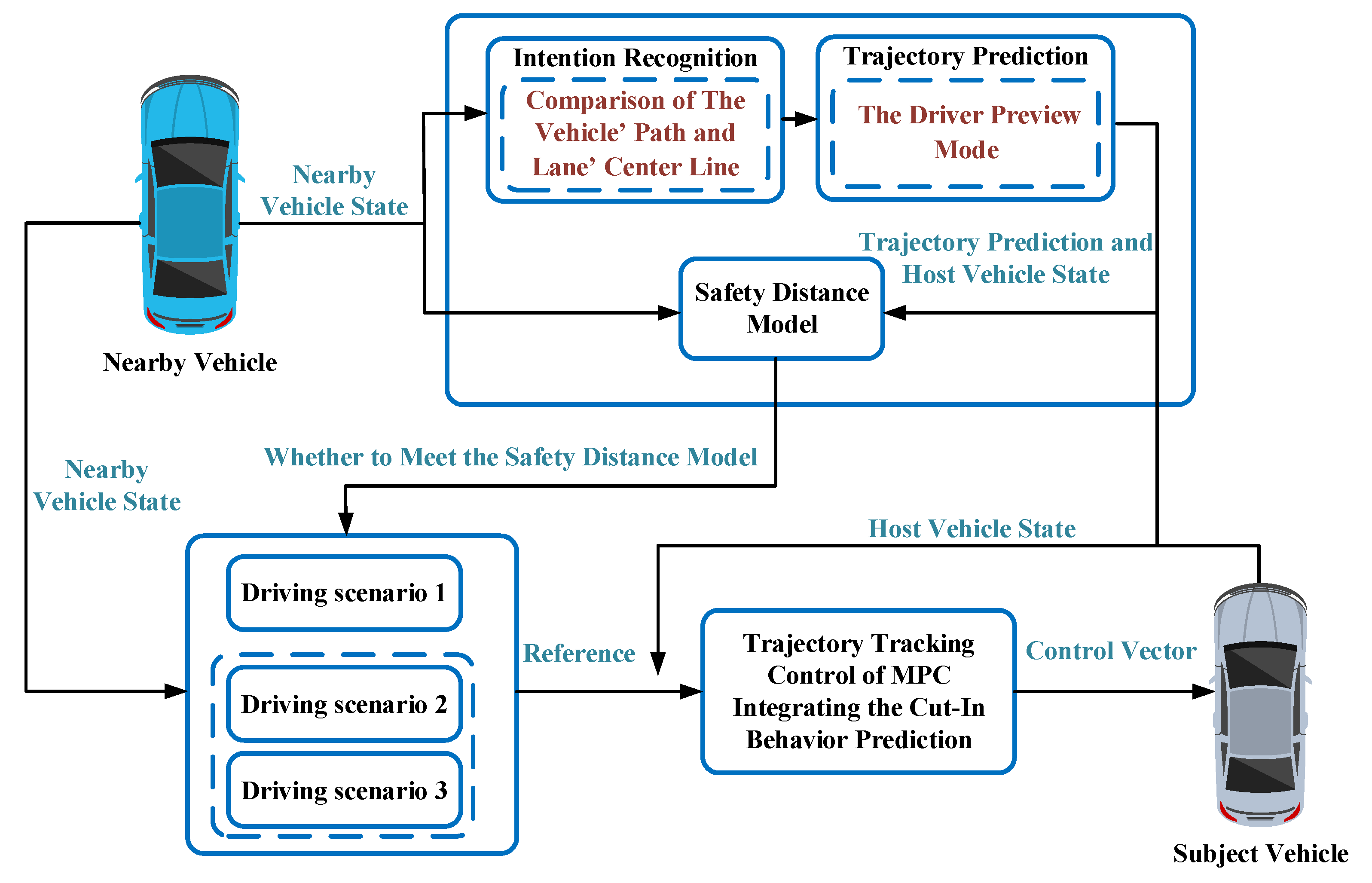
Three driving scenarios are divided according to the behavior of the adjacent vehicle, and the cut-in intention is recognized by considering similarity between the path of the adjacent vehicle and the center line of the lane where it is located. After cut-in intention recognition, the trajectory prediction method based on the driver preview model for the cut-in vehicle is proposed, which is used as a reference for subject vehicle to realize the coordinated control between the subject vehicle and the cut-in vehicle;

(2)

The safety distance model of the cut-in vehicle is proposed. Comprehensively, considering the movement state of the vehicle, the preceding vehicle ahead in the lane and the cut-in vehicle, the safety distance model of the cut-in vehicle is established, which performs the conversion of the management driving scenarios, so that the vehicle control can be taken appropriately when the cut-in vehicle changes lanes;

(3)

Facing the cut-in vehicles in different driving scenarios, cut-in prediction trajectory is integrated into a trajectory planning control method based on MPC. In the process of controlling the subject vehicle, the cut-in behavior of the adjacent vehicle is predicted and considered in advance, while ensuring the safety and driving comfort of the subject vehicle. At the same time, the subject vehicle is controlled on the optimal trajectory.

The rest of this paper is structured as follows: The cut-in scenarios division and cut-in behavior prediction are shown in Section 2, Section 3 describes the cut-in vehicle safety distance model, Section 4 introduces the trajectory tracking control method based on MPC, Section 5 The simulation result research is given, and the conclusion is obtained in Section 6.

2. Cut-In Scenarios Classification and Cut-In Behavior Prediction

According to the positional relationship between the subject vehicle, the preceding vehicle, and the cut-in vehicle, three scenarios can be divided. When an adjacent vehicle appears within the subject vehicle’s radar range, and whether it intends to change lanes to the subject vehicle’s own lane, is recognized according to the attitude of the vehicle, and then its cut-in trajectory is predicted as a reference for the subject vehicle’s trajectory tracking control.

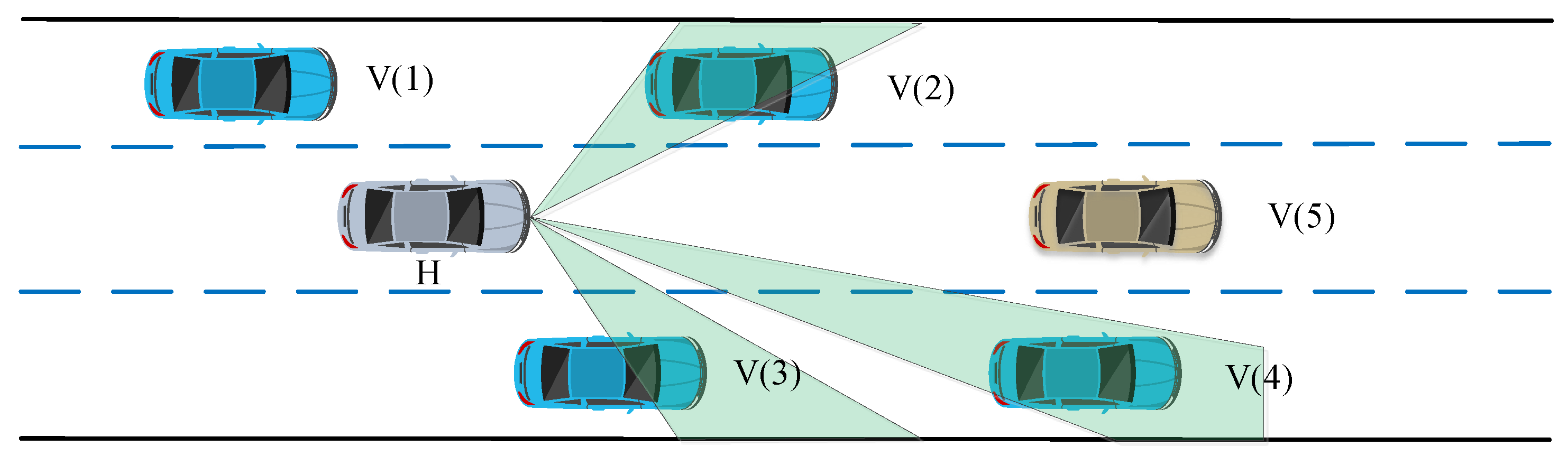
2.1. Cut-In Scenarios Classification

A more detailed scenarios division is shown in Figure 2. Driving scenarios can be divided into following the preceding vehicle, following the cut-in vehicle, and yielding the cut-in vehicle. The transition among scenarios is based on whether the cut-in vehicle exists as well as the positional relationship with the subject vehicle. The subject vehicle will adopt different control methods under different driving scenarios.

Driving scenario 1: When there is no cut-in vehicle within the radar range of the subject vehicle, or when the cut-in vehicle has completed lane changing, the subject vehicle only needs to follow the driving of the preceding vehicle. Therefore, the trajectory planning of the subject vehicle only needs to consider the preceding vehicle’s state.

Driving Scenario 2: When the adjacent vehicle is recognized by the subject vehicle to change lanes, the trajectory of the adjacent vehicle is also predicted. If its cut-in trajectory exceeds the safety distance where the relative distance between the subject vehicle and the preceding vehicle meets the cut-in vehicle safety distance model, the driving scenario is switched to following the cut-in vehicle. At this time, the trajectory planning of the subject vehicle does not need to consider the cut-in vehicle, nor does it require a control response to the cut-in maneuver of the adjacent vehicle. Only when the cut-in vehicle reaches the center line of the subject vehicle’s own lane, the subject vehicle will switch the following target from the preceding vehicle to the cut-in vehicle. At this time, the state of the cut-in vehicle will be used as a reference for the subject vehicle trajectory planning.

Driving scenario 3: When the lane-changing intention of the adjacent vehicle is recognized, and according to the predicted trajectory of the vehicle, if its cut-in trajectory is within safe distance that the relative distance between the subject vehicle and the preceding vehicle does not meet the safe distance model of the cut-in vehicle, the driving scene is transformed to yielding the cut-in vehicle. At this time, before the cut-in vehicle enters the subject vehicle’s own lane, the subject vehicle needs to use the predicted trajectory of the cut-in vehicle as a reference for its own trajectory planning, so that the subject vehicle can take control actions in advance to yield to the cut-in vehicle. As the adjacent vehicle cuts in, the subject vehicle gradually slows down through smooth control actions to provide sufficient lane change space for the adjacent vehicle. When the cut-in vehicle completes the lane change, the main vehicle also happens to follow the cut-in vehicle steadily.

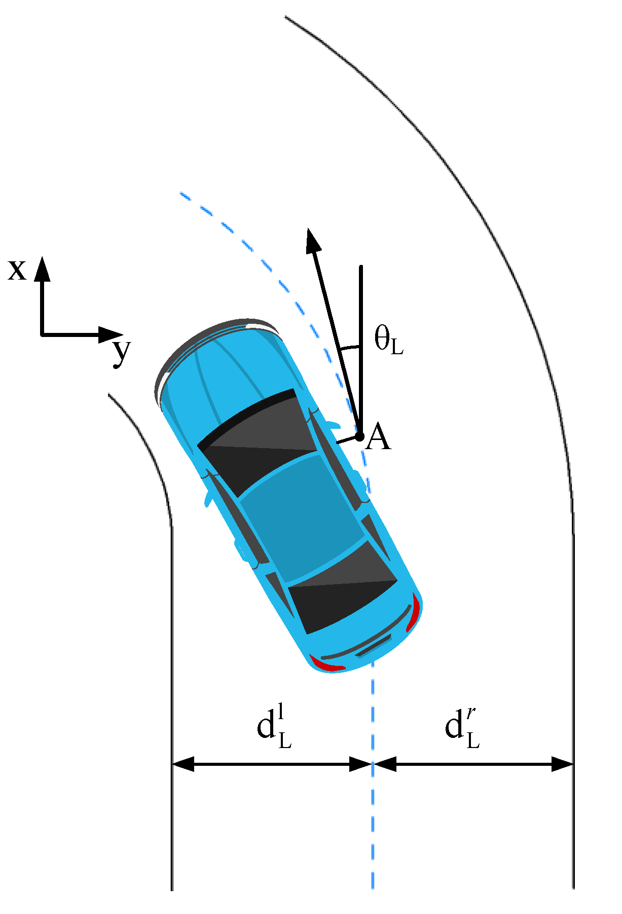
2.2. Cut-In Intention Recognition

In the cut-in scenario, an adjacent vehicle changes lanes from the original lane to the front of the subject vehicle, which is considered as the cut-in behavior of the vehicle. Therefore, according to the attitude of the adjacent vehicle when changing lanes and its road characteristics, its cut-in intention can be judged. The cut-in intention recognition method in this section is inspired by the study [27]. By comparing the relationship between the path of the cut-in vehicle and its lane, the lane-changing behavior of the adjacent vehicle and its target lane are judged. If the target lane where the adjacent vehicle changes lanes is the subject vehicle’s own lane, then this vehicle will be considered as a cut-in vehicle. Its trajectory prediction will be discussed in the next section.

As shown in Figure 3, all vehicles in the two adjacent lanes within the range of the sensor in front of the subject vehicle are judged as potential cut-in vehicles, that is vehicle 2, vehicle 3, and vehicle 4 in Figure 3.

The next analysis of the adjacent vehicle is all specifically referring to the potential cut-in vehicle. In order to determine whether the adjacent vehicle performs the lane-changing behavior, this paper quantifies the similarity between the path of the adjacent vehicle and the center line of the lane where it is located. The path of the adjacent vehicle is modeled as a circular arc as shown in Figure 4. It is assumed that all the variables of the adjacent vehicle’s attitude can be obtained by the subject vehicle’s sensor.

The vehicle path arc is defined as

$${\mathit{X}}_P={\left[d_P^l,d_P^r,{\theta }_P,{\gamma }_P\right]}^T,$$

(1)

where $d_P^l$ and $d_P^r$ are the distances from the adjacent vehicle to both sides of the lane, ${\theta }_P$ is the heading angle of the vehicle, and ${\gamma }_P$ is the curvature of the current path of the vehicle. ${\gamma }_P$ can be obtained by Equation (2)

$$\gamma =\frac{\omega }{v},$$

(2)

where $\omega$ is the yaw rate of the vehicle and $v$ is the velocity of the vehicle.

Similarly, the center line of the adjacent vehicle’s lane is also considered to be an arc, as shown in Figure 5.

The arc of the lane centerline is defined as

$${\mathit{X}}_L={\left[d_L^l,d_L^r,{\theta }_L,{\gamma }_L\right]}^T,$$

(3)

where $d_L^l$ and $d_L^r$ are both half the width of the lane, ${\theta }_L$ is the heading angle of the center line of the lane, and ${\gamma }_L$ is the curvature of the point closest to the adjacent vehicle on the center line of the lane, as shown at point A in Figure 5. Assuming that the camera of the subject vehicle can obtain the information of the centerline of the lane where the adjacent vehicle is located, the centerline is modeled as a parabolic model in the Cartesian coordinate system:

$$y(x)=a_2{x}^2+a_{1}x+a_0,$$

(4)

where $a_0$, $a_1$, and $a_2$ are both coefficients. Therefore, the heading angle ${\theta }_L$ and curvature of the lane centerline ${\gamma }_L$ are obtained:

$${\theta }_L(x)=arctan(y^{\prime }(x)),$$

(5)

$${\gamma }_L(x)=\frac{y^{″}(x)}{{(1+y^{\prime }{}^2(x))}^{\raisebox{1ex}{$3$}\!\left/ \!\raisebox{-1ex}{$2$}\right.}}.$$

(6)

The distance between the vehicle path and the centerline of the lane can be calculated by Equation (7):

$$D=\sqrt{{({\mathit{X}}_P-{\mathit{X}}_L)}^T\cdot {({\mathit{C}}_P-{\mathit{C}}_L)}^{-1}\cdot ({\mathit{X}}_P-{\mathit{X}}_L)},$$

(7)

where $D$ is the distance between the vehicle trajectory and the centerline of the lane, and $\mathit{C}$ is the covariance matrix of the vector $\mathit{X}$. In order to determine direction of the lane change of the adjacent vehicle, it is stipulated that when the vehicle path deviates to the left from the center line of the lane, the value of $D$ is positive, and when the vehicle path deviates to the right from the center line of the lane, the value of $D$ is negative, as shown in Equation (8).

$$D^{\prime }=\{\begin{array}{l}D\mathrm{Change}\mathrm{to}\mathrm{left}\mathrm{lane}\\ -D\mathrm{Change}\mathrm{to}\mathrm{right}\mathrm{lane}\end{array}.$$

(8)

During the lane change, the value of $D$ will gradually increase. On the contrary, when the vehicle enters the lane and keeps the lane, the value of $D$ will gradually decrease. Considering that the change of $D$ value is a gradual process when the vehicle is changing lane, a series of d values in the lane-changing process are weighted and averaged, assuming that the time of lane-changing is $T$, the sampling time of the system is $t_s$, the distance between the vehicle trajectory and the centerline of the lane is rewritten as

$$D_K^{*}=\frac{{\displaystyle \sum _{i=0}^{N-1}{\omega }_i{D}_{k-i}^{\prime }}}{{\displaystyle \sum _{i=0}^{N-1}{\omega }_i}},$$

(9)

$$N=\frac{T}{t_s},$$

(10)

where ${\omega }_i$ is the weight, and the earlier the sampling time is, the smaller it is.

$D_K^{*}$ is used to quantify the similarity between the path of the adjacent vehicle and the centerline of the lane. At each sampling time, $D_K^{*}$ will be recalculated based on the attitude of the adjacent vehicle. In order to determine the lane-changing intention of the adjacent vehicle, the threshold $D_{th}$ is set. The value of $D_{th}$ can be calibrated through experiments. When the absolute value $\left|D_K^{*}\right|$ of the distance is less than the threshold $D_{th}$, it is considered that the vehicle is still performing lane-keeping. When the absolute value $\left|D_K^{*}\right|$ of the distance is greater than the threshold $D_{th}$, it is considered that the vehicle is about to take a lane-changing action or that the vehicle has just entered the lane and is about to perform lane keeping. When in the first situation, the value of $D_K^{*}$ gradually increases, on the contrary, the value of $D_K^{*}$ gradually decreases when in the second situation. Therefore, the distance $D_K^{*}$ needs to be recorded after each calculation, and only when $D_K^{*}$ gradually increases, the vehicle is considered to be changing lanes.

In order to verify the reliability of cut-in intention recognition, 200 sets of lane change data at a certain velocity obtained from Carsim were selected for verification. The results are shown in

Table 1. Cut-in intention verification result.

	Left Lane Change	Right Lane Change
Detection	100%	100%
Mean time before detection	1.21 s	1.18 s

.

All the lane-changing maneuver have been detected before the vehicle reaches the intended lane. The mean time of detection is about 1 s, which is enough for subject vehicle to respond to the cut-in vehicle.

2.3. Cut-In Vehicle Trajectory Prediction

After judging the driver’s cut-in intention, the longitudinal and lateral trajectories of the cut-in vehicle need to be predicted. According to the predicted longitudinal and lateral trajectories of the cut-in vehicle, the real-time longitudinal and lateral relative positions of the cut-in vehicle and the subject vehicle can be obtained. Finally, according to the cut-in vehicle safety distance model, the trajectory of the subject vehicle needs to track can be computed. During the cut-in process of the adjacent vehicle, the driver may have fast or slow lane change behavior thanks to different driving habits [28]. The trajectory of fast and slow cut-in behavior is shown in Figure 6. Different driving behaviors will show different cut-in trajectories, so driving behavior factors need to be considered in the prediction model.

The driver’s fast or slow cut-in behavior is positively correlated with the longitudinal velocity of the cut-in vehicle. Therefore, in the prediction model, in addition to the lateral state of the adjacent vehicle, the cut-in vehicle velocity as a characterizing driving behavior also needs to be considered. Therefore, as shown in Figure 7, the driver preview model is used to predict the lateral position of the vehicle during the cut-in process, and point P on the way is the preview point. As shown in Equation (10), at each moment, the cut-in trajectory of the adjacent vehicle can be calculated by the current lateral coordinate, longitudinal velocity and yaw angle error [29], which can be measured by corner radar of the subject vehicle.

$$y_p=y_c+v_x{\theta }_{ec}\tau ,$$

(11)

where $y_p$ is the lateral position of the preview point. $y_c$ is the initial lateral position of the adjacent vehicle $v_x$ is the longitudinal velocity of the cut-in vehicle, and $\tau$ is the preview time. The yaw angle difference ${\theta }_{ec}$ represents the difference between the yaw angle of the vehicle and the yaw angle of the preview point. The preview length can be expressed as $v_x\tau$.

$${\theta }_{ec}={\theta }_P-{\theta }_d,$$

(12)

where ${\theta }_P$ is the yaw angle of the vehicle, and ${\theta }_d$ is the yaw angle of the preview point on the lane.

The parameters of the corner radar produced by BOSCH, which was used in this research, are shown in the

Table 2. Corner radar parameters.

Parameter	Value
Range Accuracy (m)	±0.02
Detection Sensitivity Range (m)	120
Azimuth Field of View (°)	140
Angle Accuracy (deg)	±0.3
Doppler Accuracy (m/s)	±0.02

. The Doppler accuracy is 0.02 m/s and the range accuracy is ±0.02 m, which have the relatively high accuracy in engineering applications.

Based on Equation (11), the lateral trajectory of the cut-in vehicle can be predicted and used as the reference of trajectory tracking control for the subject vehicle. According to the horizontal and vertical trajectory of the cut-in vehicle, when the cut-in vehicle, the preceding vehicle, and the subject vehicle do not meet the safety distance model, the vehicle will follow the lateral and longitudinal predicted trajectory of the cut-in vehicle, so that before the cut-in vehicle reaches the target lane, it brakes and follows stably in advance the cut-in vehicle, which makes a smooth transition from following the preceding vehicle to following the cut-in vehicle.

3. The Cut-In Vehicle Safety Distance Model

In daily driving, facing the cut-in behavior of the adjacent vehicle the decision of the subject vehicle will be directly affected by the relative distance $d_{rel}$ between the subject vehicle and the preceding vehicle. On the one hand, when $d_{rel}$ is large enough, as shown in Figure 8, there is enough cut-in space for the adjacent vehicle, so the cut-in maneuver of the adjacent vehicle will not affect the subject vehicle, and the subject vehicle does not need to brake in advance but switches to the following target after the adjacent vehicle cuts in. On the other hand, when $d_{rel}$ is small, as shown in Figure 9, as the cut-in possibility becomes higher and higher, in order to ensure driving safety before the adjacent vehicle cuts in, the necessary braking measures must be taken to provide enough space for the adjacent vehicle to cut in smoothly. Therefore, it is necessary to determine a minimum safe distance value to judge whether the cut-in of the adjacent vehicle will affect the normal driving of the subject vehicle.

3.1. The Safe Distance Model of the Cut-In Vehicle

Figure 10 is a schematic diagram of a cut-in scenario. The cut-in vehicle L changes from the current lane to the target lane between vehicles H and P. Vehicles L, H, and P respectively represent the cut-in vehicle, the subject vehicle, and the preceding vehicle.

Suppose the start time when the cut-in vehicle L to execute the cut-in operation is t = 0. The lane change operation consists of two parts: The first part is the initialization phase in which the cut-in vehicle L spends time t_abj for the lane change successfully to adjust the longitudinal distance to other vehicles around and its own longitudinal velocity. The second part is to perform the steering operation to cut in the target Lane. The t_abj represents adjustment time of the longitudinal distance and longitudinal velocity required by the cut-in vehicle to successfully execute the lane change before starting the lane change operation.

In order to conveniently express the longitudinal and lateral distance among the involved vehicles [30], suppose that the geodetic coordinate system is as shown in Figure 10 O is the origin, the X-asis points to the direction of the vehicle, and the Y-asis that is perpendicular to the X-asis points to the target lane. Therefore, the longitudinal acceleration, longitudinal velocity, longitudinal position, and lateral position are expressed as $a_i(t),v_i(t),x_i(t)$, and $y_i(t)$, where $i\in \left\{H,L,P\right\}$. To be more precise, the longitudinal distance and the lateral distance respectively represent the distance from the point on the upper left corner of every vehicle to the origin of the coordinate system.

3.1.1. The Minimum Longitudinal Safety Distance between the Cut-In Vehicle L and the Preceding Vehicle P

As shown in Figure 11, considering the critical collision scenario, assuming that the cut-in vehicle L collides with the preceding vehicle P in front of the target lane at point c. S represents the initial lateral distance between the upper edge of the cut-in vehicle L and the lower edge of the preceding vehicle P. D means lane width.

In order to pays more attention to the relative position relationship in the longitudinal direction of the vehicles, it is assumed that the lateral acceleration of the preceding vehicle P is 0, and the lateral position is constant. Assuming that the time at the collision point c is $t_c+t_{adj}$.The collision avoidance condition between the cut-in vehicle L and the preceding vehicle P is the following formula:

$$\begin{array}{cc}{x}_L\left(t\right)<x_P\left(t\right)-l_0-w\times \sin \left(\theta \left(t\right)\right)& \forall t\in \left[t_c+t_{adj},T\right]\end{array},$$

(13)

where $x_L\left(t\right)$$x_P\left(t\right)$ is the abscissa of the cut-in vehicle and the preceding vehicle, respectively, $l_0$ is the average length of passage vehicles, and $\theta (t)$ is the yaw angle of the vehicle when changing lanes.

The last term in Formula (13) represents the distance between the cut-in vehicle L and the preceding vehicle P in the interval of $\left[t_c+t_{adj},t_{lat}+t_{adj}\right]$ to avoid collision. The calculation is as follows:

$$\tan \left(\theta \left(t\right)\right)=\frac{v_{lat}\left(t\right)}{v_L\left(t\right)},$$

(14)

where $v_{lat}\left(t\right)$ is the lateral velocity of the cut-in vehicle, $v_L\left(t\right)$ is the longitudinal velocity of the cut-in vehicle. The largest $\theta (t)$ that is the largest $sin(\theta (t))$ is obtained at the $t=t_c+t_{adj}$ moment. Defining $L_P=l_0+W\times sin(\theta (t_c+t_{adj}))$, the above formula is simplified to

$$\begin{array}{cc}{x}_L\left(t\right)<x_P\left(t\right)-L_P& \forall t\in \left[t_c+t_{adj},T\right]\end{array}.$$

(15)

Use $S_r\left(t\right)$ to represent the longitudinal distance between the cut-in vehicle L and the preceding vehicle P during the lane change.

$$\begin{array}{cc}{S}_r\left(t\right)=x_P\left(t\right)-L_P-x_L\left(t\right)& \forall t\in \left[t_c+t_{adj},T\right]\end{array}.$$

(16)

In order to make the cut-in vehicle L not collide with the preceding vehicle P during the lane change process, the following equation needs to be satisfied:

$$\begin{array}{cc}{S}_r\left(t\right)=\left(\begin{array}{l}{S}_r\left(0\right)+{\displaystyle {\int }_0^t{\displaystyle {\int }_0^{\lambda }\left(a_P\left(\tau \right)-a_L\left(\tau \right)\right)}}d\tau d\lambda +\\ \left(v_P\left(0\right)-v_L\left(0\right)\right)\times t\end{array}\right)>0& \forall t\in \left[t_c+t_{adj},T\right]\end{array},$$

(17)

where $S_r\left(0\right)=x_P\left(0\right)-l_0-x_L\left(0\right)$. In order not to collide with the preceding vehicle P, the longitudinal distance $S_r\left(t\right)$ between the cut-in vehicle L and the preceding vehicle P should be as large as possible during the period of $\left[t_c+t_{adj},T\right]$, and the $S_r{\left(t\right)}_{\max }$ will be used as the minimum safe distance $MSD(L,P)$ at which the cut-in vehicle L will not collide with the preceding vehicle P during the lane change process, so the $MSD(L,P)$ is obtained:

$$\begin{array}{cc}MSD\left(L,P\right)=\underset{t}{Max}\left(\begin{array}{l}{\displaystyle {\int }_0^t{\displaystyle {\int }_0^{\lambda }\left(a_L\left(\tau \right)-a_P\left(\tau \right)\right)}}d\tau d\lambda +\\ \left(v_L\left(0\right)-v_P\left(0\right)\right)\times t+l_0\end{array}\right)& \forall t\in \left[t_c+t_{adj},T\right]\end{array},$$

(18)

where $a_L$ is the longitudinal acceleration of the cut-in vehicle, $a_P$ is the longitudinal acceleration of the preceding vehicle, $v_L$ is the longitudinal velocity of the cut-in vehicle, $v_P$ is the longitudinal velocity of the preceding vehicle.

3.1.2. The Minimum Longitudinal Safety Distance between the Cut-In Vehicle L and the Subject Vehicle H

As shown in Figure 12, considering the critical collision scenario, assuming that the cut-in vehicle L collides with the subject vehicle H at point c. S represents the initial lateral distance between the upper edge of the cut-in vehicle L and the lower edge of the subject vehicle H. D means lane width.

The lateral acceleration of the subject vehicle H is 0 and the lateral position is constant. Assuming that the moment at the collision point c is $t_c+t_{adj}$, in order to avoid collision between the cut-in vehicle L and the subject vehicle H, the following equation needs to be satisfied:

$$\begin{array}{cc}{x}_H\left(t\right)<x_L\left(t\right)-l_0\times \cos \left(\theta \left(t\right)\right)& \forall t\in \left[t_c+t_{adj},T\right]\end{array},$$

(19)

where $x_P\left(t\right)$ is the abscissa of the subject vehicle, $l_0$ is the length of vehicles.

Ignoring the influence of vehicle yaw [31], the above formula can be simplified to the following formula:

$$\begin{array}{cc}{x}_H\left(t\right)<x_L\left(t\right)-l_0& \forall t\in \left[t_c+t_{adj},T\right]\end{array}.$$

(20)

Use $S_r\left(t\right)$ to represent the longitudinal distance between the cut-in vehicle L and the subject vehicle H during the lane change.

$$\begin{array}{cc}{S}_r\left(t\right)=x_L\left(t\right)-L-x_H\left(t\right)& \forall t\in \left[t_c+t_{adj},T\right]\end{array}.$$

(21)

In order to make the cut-in vehicle L not collide with the subject vehicle H during the lane change process, the following equation needs to be satisfied:

$$\begin{array}{cc}{S}_r\left(t\right)=\left(\begin{array}{l}{S}_r\left(0\right)+{\displaystyle {\int }_0^t{\displaystyle {\int }_0^{\lambda }\left(a_L\left(\tau \right)-a_H\left(\tau \right)\right)}}d\tau d\lambda +\\ \left(v_L\left(0\right)-v_H\left(0\right)\right)\times t\end{array}\right)>0& \forall t\in \left[t_c+t_{adj},T\right]\end{array},$$

(22)

where $S_r\left(0\right)=x_L\left(0\right)-l_0-x_H\left(0\right)$, the minimum safety distance $MSD(L,H)$ at which the cut-in vehicle L will not collide with the subject vehicle P during the lane change process is obtained.

$$\begin{array}{cc}MSD\left(L,H\right)=\underset{t}{Max}\left(\begin{array}{l}{\displaystyle {\int }_0^t{\displaystyle {\int }_0^{\lambda }\left(a_H\left(\tau \right)-a_L\left(\tau \right)\right)}}d\tau d\lambda \\ +\left(v_H\left(0\right)-v_L\left(0\right)\right)\times t+l_0\end{array}\right)& \forall t\in \left[t_c+t_{adj},T\right]\end{array},$$

(23)

where $a_H$ is the longitudinal acceleration of the subject vehicle, $v_H$ is the longitudinal velocity of the subject vehicle.

4. Trajectory Tracking Control

The model predictive control is adopted in this section to track the reference trajectory. After identifying the cut-in intention of the adjacent vehicle and predicting the trajectory, the safety distance model of the cut-in vehicle is compared with the relative distance between the subject vehicle and the preceding vehicle. If the current relative distance satisfies the safety distance model, only the longitudinal trajectory of the cut-in vehicle is used as the reference trajectory for the subject vehicle trajectory tracking. On the contrary, if the current relative distance does not meet the safety distance model, then the longitudinal and lateral trajectories of the cut-in vehicle are used as the reference for trajectory tracking to ensure that as the nearby enters, the main vehicle can gradually decelerate so that there is enough space provided to change lanes for the cut-in vehicle. While ensuring the safety between the subject vehicle and the cut-in vehicle, the subject vehicle can obtain a smoother process.

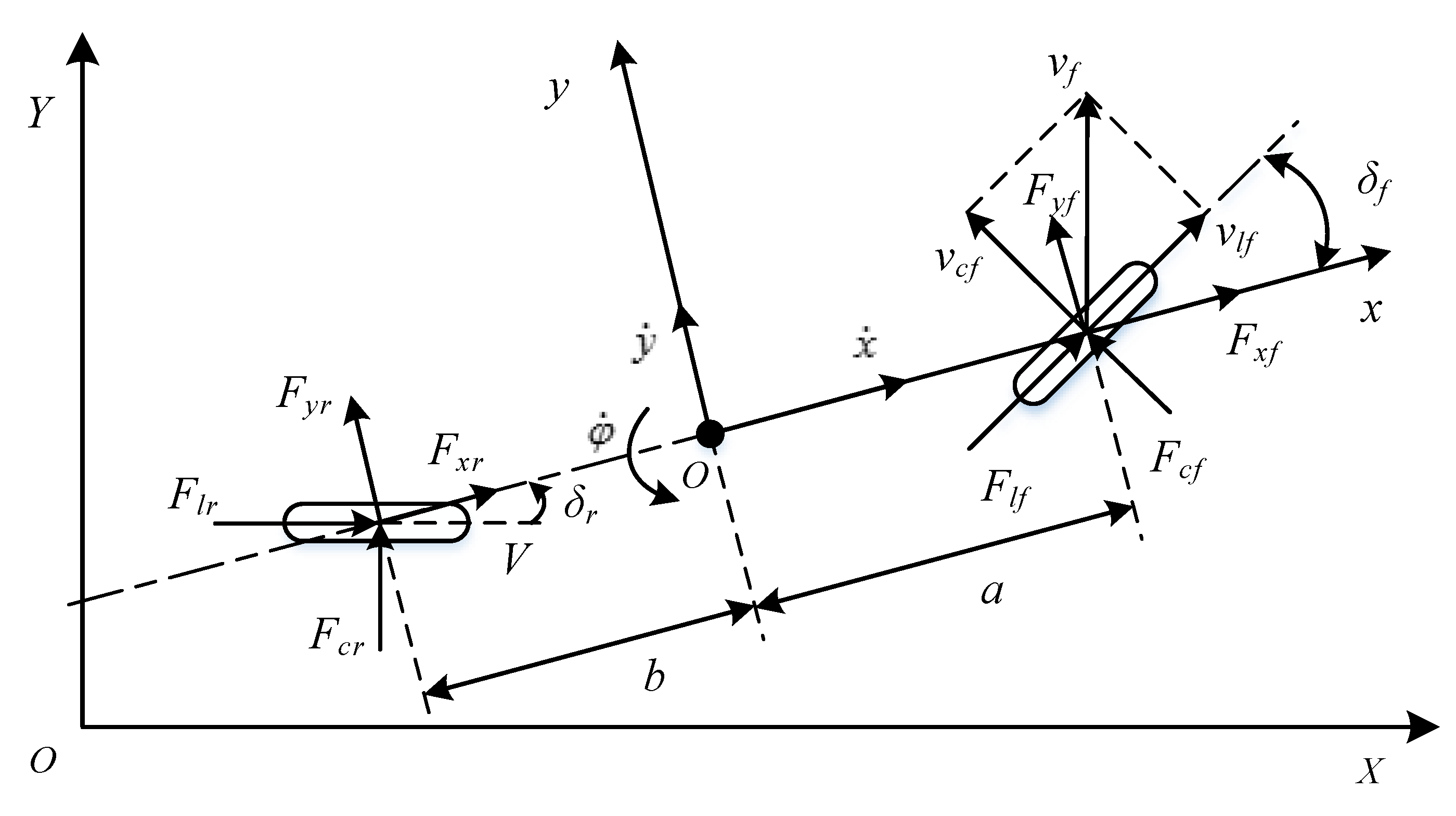
4.1. Subject Vehicle Model

The bicycle model is used for the design of the model predictive controller. The longitudinal, lateral, and yaw motions of the vehicle are considered [32], while the pitch and roll motions are ignored. The bicycle model is shown in Figure 13 below.

The force balance equation along the coordinate axis is listed:

$$m\ddot{x}=m\dot{y}\dot{\phi }+2{\mathit{F}}_{xf}+2{\mathit{F}}_{xr},$$

(24)

$$m\ddot{y}=-m\dot{x}\dot{\phi }+2{\mathit{F}}_{yf}+2{\mathit{F}}_{yr},$$

(25)

$$I_z\ddot{\phi }=2a{\mathit{F}}_{yf}-2b{\mathit{F}}_{yr},$$

(26)

where $m$ is mass of vehicle, ${\mathit{F}}_{xf}$ and ${\mathit{F}}_{xr}$ are the x-direction forces of wheels, ${\mathit{F}}_{yf}$ and ${\mathit{F}}_{yr}$ are the y-direction forces of wheels, $a$ and $b$ are the distance from vehicle center of gravity to its front and rear axles, $m$ is the mass of the vehicle, and $I_z$ is the moment of inertia of the vehicle around the Z-asis.

The simplified nonlinear model of vehicle dynamics is as follows:

$$\begin{array}{l}m\ddot{y}=-m\dot{x}\dot{\phi }+2\left[C_{cf}\left({\delta }_f-\frac{\dot{y}+a\dot{\phi }}{\dot{x}}\right)+C_{cr}\frac{b\dot{\phi }-\dot{y}}{\dot{x}}\right]\\ m\ddot{x}=m\dot{y}\dot{\phi }+2\left[C_{lf}{s}_f+C_{cf}\left({\delta }_f-\frac{\dot{y}+a\dot{\phi }}{\dot{x}}\right){\delta }_f+C_{lr}{s}_r\right]\\ I_z\ddot{\phi }=2\left[a{C}_{cf}\left({\delta }_f-\frac{\dot{y}+a\dot{\phi }}{\dot{x}}\right)-b{C}_{cr}\frac{b\dot{\phi }-\dot{y}}{\dot{x}}\right]\\ \dot{Y}=\dot{x}\sin \phi +\dot{y}\cos \phi \\ \dot{X}=\dot{x}\cos \phi -\dot{y}\sin \phi \end{array}$$

(27)

where $C_l$ is the tire longitudinal stiffness, and $C_c$ is the tire cornering stiffness, $s$ is the tire slip rate, $\alpha$ is the tire slip angle, $\delta$ is the tire deflection angle.

In this system, the state quantity ${\xi }_{dyn}={\left[\dot{y},\dot{x},\phi ,\dot{\phi },Y,X\right]}^T$ is selected as 1, and the control quantity is $u_{dyn}={\delta }_f$. That is, the longitudinal velocity of the vehicle is assumed to be unchanged during the control process, and only the front wheel angle of the vehicle is controlled. Because the MPC does not have high real-time performance for the nonlinear model, it is necessary to linearize the nonlinear model.

For the established nonlinear dynamic model:

$${\dot{\xi }}_{dyn}=f_{dyn}\left({\xi }_{dyn},u_{dyn}\right).$$

(28)

The state and control of the MPC reference system at any time meet the following relationship:

$${\stackrel{·}{\xi }}_r=f({\xi }_r,{\mathit{u}}_r).$$

(29)

Carry out Taylor expansion of ${\dot{\xi }}_{dyn}$ at the reference point $({\xi }_r,{\mathit{u}}_r)$ of the trajectory, and keep only the first-order terms, ignoring the higher-order terms, and get:

$${\dot{\xi }}_{dyn}=f({\xi }_r,{\mathit{u}}_r)+{\frac{\partial f}{\partial \xi }|}_{\begin{array}{l}\xi ={\xi }_r\\ \mathit{u}={\mathit{u}}_r\end{array}}(\xi -{\xi }_r)+{\frac{\partial f}{\partial \mathit{u}}|}_{\begin{array}{l}\xi ={\xi }_r\\ \mathit{u}={\mathit{u}}_r\end{array}}(\mathit{u}-{\mathit{u}}_r).$$

(30)

Formula (30) also be written as

$${\dot{\xi }}_{dyn}=f({\xi }_r,{\mathit{u}}_r)+J_f({\xi }_{dyn})({\xi }_{dyn}-{\xi }_r)+J_f(\mathit{u})(\mathit{u}-{\mathit{u}}_r),$$

(31)

where $J_f({\xi }_{dyn})$ is the Jacobian matrix of $f$ relative to $\xi$, and $J_f(\mathit{u})$ is the Jacobian matrix of $f$ relative to $\mathit{u}$. Subtracting Equations (39) and (37) can get

$${\widetilde{\stackrel{·}{\xi }}}_{dyn}={\mathit{A}}_{dyn}(t)\widetilde{{\xi }_{dyn}}+{\mathit{B}}_{dyn}(t)\tilde{\mathit{u}},$$

(32)

where ${\widetilde{\stackrel{·}{\xi }}}_{dyn}={\xi }_{dyn}-{\xi }_r$,$\tilde{\mathit{u}}=\mathit{u}-{\mathit{u}}_r$.

$${\mathit{B}}_{dyn}\left(t\right)={\frac{\partial f_{dyn}}{\partial {\mathit{u}}_{dyn}}|}_{{\widehat{\xi }}_t,u_t}=\left[\frac{2C_{cf}}{m},\frac{2C_{cf}\left(2{\delta }_{f,t-1}-\frac{{\dot{y}}_t+a{\dot{\phi }}_t}{{\dot{x}}_t}\right)}{m},0,\frac{2a{C}_{cf}}{I_z},0,0\right],$$

$$\begin{array}{l}{\mathit{A}}_{dyn}\left(t\right)={\frac{\partial f_{dyn}}{\partial {\xi }_{dyn}}|}_{{\widehat{\xi }}_t,{\mathit{u}}_t}\\ =\left[\begin{array}{cccccc}-\frac{2\left(C_{cf}+C_{cr}\right)}{m{\dot{x}}_t}& \frac{\partial f_{\dot{y}}}{\partial \dot{x}}& 0& -{\dot{x}}_t+\frac{2\left(b{C}_{cr}-a{C}_{cf}\right)}{m{\dot{x}}_t}& 0& 0\\ \dot{\phi }-\frac{2C_{cf}{\delta }_{f,t-1}}{m{\dot{x}}_t}& \frac{\partial f_{\dot{x}}}{\partial \dot{x}}& 0& {\dot{y}}_t-\frac{2a{C}_{cf}{\delta }_{f,t-1}}{m{\dot{x}}_t}& 0& 0\\ 0& 0& 0& 1& 0& 0\\ \frac{2\left(b{C}_{cr}-a{C}_{cf}\right)}{I_z{\dot{x}}_t}& \frac{\partial f_{\dot{\phi }}}{\partial \dot{x}}& 0& -\frac{2\left(a^2{C}_{cf}+b^2{C}_{cr}\right)}{I_z{\dot{x}}_t}& 0& 0\\ \cos \left({\phi }_t\right)& sin\left({\phi }_t\right)& {\dot{x}}_t\cos \left({\phi }_t\right)-{\dot{y}}_{t}sin\left({\phi }_t\right)& 0& 0& 0\\ -sin\left({\phi }_t\right)& \cos \left({\phi }_t\right)& -{\dot{y}}_t\cos \left({\phi }_t\right)-{\dot{x}}_{t}sin\left({\phi }_t\right)& 0& 0& 0\end{array}\right]\end{array}$$

where

$$\frac{\partial f_{\dot{y}}}{\partial \dot{x}}=\left(2C_{cf}\left({\dot{y}}_t+a{\dot{\phi }}_t\right)+2C_{cr}\left({\dot{y}}_t-b{\dot{\phi }}_t\right)\right)/m{\dot{x}}_t^2-{\dot{\phi }}_t,$$

$$\frac{\partial f_{\dot{x}}}{\partial \dot{x}}=\left(2C_{cf}{\delta }_{f,t-1}\left({\dot{y}}_t+a{\dot{\phi }}_t\right)\right)/\left(m{\dot{x}}_t^2\right),$$

$$\frac{\partial f_{\dot{\phi }}}{\partial \dot{x}}=\left(2a{C}_{cf}\left({\dot{y}}_t+a{\dot{\phi }}_t\right)-2b{C}_{cr}\left({\dot{y}}_t-b{\dot{\phi }}_t\right)\right)/I_z{\dot{x}}_t^2.$$

Equation (32) is continuous and cannot be used for the design of model predictive controllers, so it is necessary to perform approximate discretization processing. As shown in the following formula:

$$\begin{array}{l}{\mathit{A}}_{k,t}=\mathit{I}+T\mathit{A}(t)\\ {\mathit{B}}_{k,t}=T\mathit{B}(t)\end{array}$$

(33)

According to Equation (40), the above linear dynamics model is discretized using the first-order difference quotient:

$${\xi }_{dyn}\left(k+1\right)={\mathit{A}}_{dyn}\left(k\right){\xi }_{dyn}\left(k\right)+{\mathit{B}}_{dyn}\left(k\right){\mathit{u}}_{dyn}\left(k\right),$$

(34)

where ${\mathit{A}}_{dyn}\left(k\right)=I+T{\mathit{A}}_{dyn}\left(t\right)$,${\mathit{B}}_{dyn}\left(k\right)=T{\mathit{B}}_{dyn}\left(t\right)$.

4.2. Reference Trajectory Generation

4.2.1. Driving Scenario 1

In driving scenario 1, there is no cut-in vehicle, and the subject vehicle only follows the preceding vehicle. Therefore, the reference trajectory of the subject vehicle is the longitudinal trajectory of the preceding vehicle. Considering the safety of following the vehicle, the longitudinal reference trajectory of the subject vehicle is

$$x_r(k)=x_P(k)-d_{safe}(k),$$

(35)

where $x_r(k)$ is the reference trajectory of the subject vehicle, $x_P(k)$ is the trajectory point of the preceding vehicle, and $d_{safe}(k)$ is the safe distance between the subject vehicle and the preceding vehicle, which can be calculated:

$$d_{safe}(k)=\stackrel{·}{x}(k)t_{th}+d_0,$$

(36)

where $t_{th}$ is the time headway, $d_0$ is the minimum distance.

In order to make the subject vehicle follow the preceding vehicle stably, the longitudinal reference velocity of the main vehicle is

$${\stackrel{·}{x}}_r(k)={\stackrel{·}{x}}_P(k),$$

(37)

where ${\stackrel{·}{x}}_P(k)$ is velocity of the preceding vehicle.

Since the subject vehicle is driving along the own lane, the lateral reference trajectory $y_r(k)$, lateral velocity ${\stackrel{·}{y}}_r(k)$, yaw angle ${\phi }_r(k)$, and yaw angle velocity ${\stackrel{·}{\phi }}_r(k)$ are all 0, as shown in the following formula:

$$\begin{array}{l}{y}_r(k)=0\hspace{1em}{\stackrel{·}{y}}_r(k)=0\\ {\phi }_r(k)=0\hspace{1em}{\stackrel{·}{\phi }}_r(k)=0\end{array}$$

(38)

Therefore, in driving scenario 1, the reference trajectory of the subject vehicle trajectory tracking is

$${\xi }_r={[0,{\stackrel{·}{x}}_P,0,0,0,x_P(k)-d_{safe}(k)]}^T,$$

(39)

$${\mathit{u}}_r=[0].$$

(40)

4.2.2. Driving Scenario 2

In driving scenario 2, the cut-in intention and cut-in trajectory of the adjacent vehicle are recognized. However, because the relative distance between the subject vehicle and the preceding vehicle is greater than the safety distance model of the cut-in vehicle, there is enough lane-changing space for the adjacent vehicle to cut in. In this scenario, when the subject vehicle changes lanes to the center line of the subject vehicle’s own lane, the subject vehicle needs to take the cut-in vehicle as the follow-up target. Therefore, similarly, the subject vehicle longitudinal reference trajectory $x_r(k)$ and longitudinal reference velocity ${\stackrel{·}{x}}_r(k)$ are

$$x_r(k)=x_L(k)-d_{safe}(k),$$

(41)

$${\stackrel{·}{x}}_r(k)={\stackrel{·}{x}}_L(k).$$

(42)

The lateral reference trajectory $y_r(k)$, lateral velocity ${\stackrel{·}{y}}_r(k)$, yaw angle ${\phi }_r(k)$, and yaw angle velocity ${\stackrel{·}{\phi }}_r(k)$ are all 0. Therefore, the trajectory tracking reference trajectory in driving scenario 2 is

$${\xi }_r={[0,{\stackrel{·}{x}}_L,0,0,0,x_L(k)-d_{safe}(k)]}^T,$$

(43)

$${\mathit{u}}_r=[0].$$

(44)

4.2.3. Driving Scenario 3

In driving scenario 3, because the relative distance between the subject vehicle and the preceding vehicle does not satisfy the cut-in vehicle safety distance model, once the cut-in intention of the adjacent vehicle is recognized, its predicted trajectory immediately becomes the reference trajectory of the subject vehicle. Moreover, as the adjacent vehicle cuts in, the subject vehicle needs to gradually slow down to provide it with lane-changing space. Therefore, the subject vehicle needs to use both the longitudinal predicted trajectory and the horizontal predicted trajectory of the nearby as a reference. The lateral predicted trajectory of the adjacent vehicle is merged into the longitudinal predicted trajectory [33] as the reference for the longitudinal trajectory of the subject vehicle, so the longitudinal reference trajectory of the main vehicle is

$$x_r(k)=x_L(k)-d_{safe}(k)+\frac{L-y_L(k)}{L_0}(d_{safe}(k)-d_0),$$

(45)

where is the initial relative distance between the subject vehicle and the adjacent vehicle, $L$ is the width of the road line, and $L_0$ is the distance from the adjacent vehicle to the center line of the vehicle’ lane at the initial moment. $y_L(k)$ is the predicted trajectory of the adjacent vehicle, which is calculated as according to Equation (11):

$$y_c(k+1)=y_c(k)+v_P(k){\theta }_{ec}(k)T_s,$$

(46)

where $v_P(k)$ is the longitudinal velocity of the adjacent vehicle and ${\theta }_{ec}(k)$ is the difference in yaw angle.

Since in driving scene 3, the subject vehicle is not following the cut-in vehicle, there is no reference for the longitudinal velocity. Therefore, ${\stackrel{·}{x}}_r(k)=0$. Similarly, t the lateral reference trajectory $y_r(k)$, lateral velocity ${\stackrel{·}{y}}_r(k)$, yaw angle ${\phi }_r(k)$, and yaw angle velocity ${\stackrel{·}{\phi }}_r(k)$ are all 0. Therefore, the trajectory tracking reference in driving scenario 3 is

$${\xi }_r={[0,0,0,0,0,x_L(k)-d_{safe}(k)+\frac{L-y_L(k)}{L_0}(d_{safe}(k)-d_0)]}^T,$$

(47)

$${\mathit{u}}_r=[0].$$

(48)

4.3. Main Vehicle Objective Function and Constraint Establishment

The control purpose of MPC is that the subject vehicle can follow the reference trajectory when the constraints are met. Therefore, the objective function of the main vehicle is

$$J={{\displaystyle \sum _{i=1}^p\Vert {\mathit{W}}_1{\xi }_{dyn}(k+i|k)\Vert }}^2+{{\displaystyle \sum _{i=1}^{m-1}\Vert {\mathit{W}}_2\mathit{u}(k+i)\Vert }}^2,$$

(49)

where ${\mathit{W}}_1$ and ${\mathit{W}}_2$ are coefficient matrices, and $p$ is the prediction horizon. $m$ is the control horizon, $p>m$.

When solving the optimization problem of MPC, various constraints also need to be satisfied [34]. First of all, in order to ensure the driving safety of the subject vehicle during the following process, the longitudinal relative distance between the subject vehicle and the preceding vehicle or the cut-in vehicle must meet the minimum safety distance constraint:

$$x(k)\ge d_c,$$

where $d_c$ is the minimum safety distance.

In addition, the constraints of the subject vehicle dynamics considered are as follows:

$$\begin{array}{l}{v}_{x\min }\le \stackrel{·}{x}(k)\le v_{x\max }\\ \stackrel{·}{y}(k)\le v_{y\max }\\ \left|{\delta }_f(k)\right|\le {\delta }_{\max }\end{array}$$

Finally, the optimization problem of trajectory tracking based on MPC can be expressed as

$$\underset{U(k)}{\min }J(\mathit{x}(k),\mathit{u}(k)).$$

(50)

Subject to

$$\begin{array}{l}x(k)\ge d_c\\ v_{x\min }\le \stackrel{·}{x}(k)\le v_{x\max }\\ \stackrel{·}{y}(k)\le v_{y\max }\\ \left|{\delta }_f(k)\right|\le {\delta }_{\max }\end{array}$$

where

$$J={{\displaystyle \sum _{i=1}^p\Vert {\mathit{W}}_1{\xi }_{dyn}(k+i|k)\Vert }}^2+{{\displaystyle \sum _{i=1}^{m-1}\Vert {\mathit{W}}_2\mathit{u}(k+i)\Vert }}^2.$$

5. Simulation Results and Analysis

The trajectory tracking control method provided in this article was verified by the Simulink platform. According to the driving scenario division, the trajectory tracking strategy in different scenarios was simulated and verified. This article adopted a scene in which an adjacent vehicle in the adjacent lane cut int the front of the subject vehicle on an urban road.

5.1. Driving Scenario 1

In driving scenario 1, the vehicle in the adjacent lane does not perform the cut-in behavior, and the subject vehicle is following the preceding vehicle at this time. The subject vehicle will use the longitudinal displacement and velocity of the preceding vehicle in as the reference for trajectory tracking. The longitudinal velocity and the relative distance of the vehicles are shown in Figure 14.

In Figure 14, the vehicle can take the longitudinal trajectory and velocity of the preceding vehicle as a reference, and followed the preceding vehicle steadily. Since there was no cut-in vehicle, the vehicle would adopt corresponding velocity control after recognizing the existence of the preceding vehicle to maintain a consistent velocity and a safe relative distance. In Figure 14a, the initial velocity of the subject vehicle was 60 km/h. After detecting the presence of the preceding vehicle at time 0, it started to decelerate, and gradually coincided with the velocity of the vehicle in front after 10 s. The relative distance between the vehicle and the vehicle in front, as shown in Figure 14b, gradually decreased from the initial 40 m to 31 m, and remained unchanged.

5.2. Driving Scenario 2

In driving scenario 2, the vehicle in the adjacent lane has a potential to cut in the front of the subject vehicle, but the relative distance between the subject vehicle and the preceding vehicle meets the safety distance model of the cut-in vehicle, so the subject vehicle does not need to brake in advance. When the cut-in vehicle enters the lane of the subject vehicle, the subject vehicle switches into the vehicle as the follow-up target, and adopts the corresponding velocity control to complete the following the cut-in vehicle.

In Figure 15, the vehicle steadily followed the preceding vehicle and maintained the relative distance of 43 m unchanged. The cut-in vehicle started to cut in at a velocity of 53 km/h at 26 s, as shown in Figure 15a. When the adjacent vehicle L cut in, the relative distance between the subject vehicle H and the preceding vehicle P satisfies the cut-in vehicle safety distance model. Before the vehicle cut in, no braking measures had been taken by the subject vehicle. As shown in Figure 15b, after the vehicle detected the cut-in behavior of the adjacent vehicle in 26 s, the vehicle switched the following target to the cut-in vehicle, and the subject vehicle velocity decelerates from 60 km/h to 53 km/h. As shown in Figure 15c, when the subject vehicle took the cut-in vehicle as the follow-up target, the relative distance suddenly changed to 35m, and then it steadily follows the cut-in vehicle.

5.3. Driving Scenario 3

In driving scenario 3, there is a potential cut-in vehicle in the adjacent lane and the relative distance did not satisfy the cut-in vehicle safety distance model. Therefore, the subject vehicle needed to yield to the cut-in vehicle to provide a sufficient relative distance for the vehicle to change lanes, so as to prevent the vehicle from emergency braking or even a collision with the cut-in vehicle.

In the initial stage, the subject vehicle followed the preceding vehicle steadily. The adjacent vehicle started to cut-in at a velocity of 60 km/h in 26 s. According to Figure 16a, the relative distance between the subject vehicle and the preceding vehicle is constant distance of 32 m, which did not meet the cut-in vehicle safety distance model. According to Figure 16b, as the attitude of the adjacent vehicle changed, the subject vehicle had recognized the cut-in intention of the adjacent vehicle at 20 s and gradually slowed down. As shown in Figure 16c, due to the early braking of the subject vehicle, the relative distance between the subject vehicle and the preceding vehicle increased. This made the relative distance 48 m when the adjacent vehicle performed the behavior in 26 s, which satisfied the cut-in vehicle safety distance model. At the same time, the vehicle switched the following target to the cut-in vehicle, and the relative distance suddenly changed to 32 m, which is close to a stable following distance. In the end, the velocity of the subject vehicle is the same as that of the cut-in vehicle, and the relative distance reached the expected following distance. Finally, the subject vehicle followed the cut-in vehicle steadily. In Figure 16, compared with the subject vehicle without the cut-in behavior prediction, the subject vehicle with the cut-in behavior prediction obtained a smaller deceleration due to early braking, and at the same time avoided the sudden decrease in the relative distance caused by the sudden lane-changing of the cut-in vehicle, which made the subject vehicle obtain a smoother control process, when facing a vehicle cutting in.

5.4. Method Application Evaluation

Considering the engineering applicability of the method mentioned in the paper, the computational complexity of the method needs to be evaluated. The simulation test of driving scenario 3 was selected to calculate the complexity of the method.

As shown in

Table 3. The computational complexity of the method in driving scenario 3.

Variables	Value
Simulation termination time (s)	100
Simulation step (s)	0.02
Actual simulation time (s)	54.67
RAM (MB)	9286

, the simulation termination time was set to 100 s and the simulation step was set to 0.02 s, which was obtained by repeated tests. But in fact, the system only took 54.67 s to run. The RAM is 9286 MB during the running of the method, which can be loaded by the controller of vehicle and is suitable for real-time applications in engineering.

6. Conclusions

For intelligent vehicles, this paper proposed a trajectory tracking control method based on cut-in behavior prediction. Considering the cut-in vehicles, the three driving scenarios were divided in this paper. In different scenarios, the attitude of the adjacent vehicle was compared with the center line of the lane to judge the cut-in intention of the adjacent vehicle. The driving preview model was adopted to predict the cut-in trajectory. The safety distance model of the cut-in vehicle was established to judge the switching of scenarios. The cut-in vehicle trajectory in different scenarios was used as a reference for MPC trajectory tracking control of the subject vehicle. MPC is used to solve the optimal control trajectory of the subject vehicle under different reference trajectories. When facing lane change of the adjacent vehicle, the subject vehicle can follow the cut-in vehicle safely and comfortably. The trajectory tracking control method proposed in the paper was confirmed by the Simulink platform. Finally, the computational complexity was evaluated to prove the practically feasibility of the method proposed in this paper. For future research, more cut-in behaviors in different road scenarios will be considered and investigated. Moreover, experimental confirmations will be conducted.

References

1. Yang, J.; Coughlin, J.F. In-vehicle technology for self-driving cars: Advantages and challenges for aging drivers. Int. J. Automot. Technol. 2014, 15, 333–340. [Google Scholar] [CrossRef]
2. Yoshida, H.; Omae, M.; Wada, T. Toward next active safety technology of intelligent vehicle. J. Robot. Mechatron. 2015, 27, 610–616. [Google Scholar] [CrossRef]
3. Hu, C.; Wang, R.; An, F.Y.; Chen, N. Output constraint control on path following of four-wheel independently actuated intelligent ground vehicles. IEEE Trans. Veh. Technol. 2016, 65, 4033–4043. [Google Scholar] [CrossRef]
4. Chen, C.P.; Guo, J.H.; Guo, C. Adaptive Cruise Control for Cut-In Scenarios Based on Model Predictive Control Algorithm. Appl. Sci. 2021, 11, 5293. [Google Scholar] [CrossRef]
5. Kumar, P.; Perrollaz, M.; Lefevre, S.; Laugier, C. Learning-Based Approach for Online Lane Change Intention Prediction. In Proceedings of the 2013 IEEE Intelligent Vehicles Symposium, Gold Coast City, QLD, Australia, 23–26 June 2013. [Google Scholar]
6. Kim, I.H.; Bong, J.H.; Park, J.; Park, S. Prediction of driver’s intention of lane change by augmenting sensor information using machine learning techniques. Sensors 2017, 17, 1350. [Google Scholar] [CrossRef] [PubMed] [Green Version]
7. Liu, P.; Kurt, A.; Redmill, K.; Ozguner, U. Classification of Highway Lane Change Behavior to Detect Dangerous Cut-in Maneuvers. In Proceedings of the Transportation Research Board (TRB) 95th Annual Meeting, Washington, DC, USA, 10–14 January 2016. [Google Scholar]
8. Jo, K.; Lee, M.; Kim, J.; Sunwoo, A. Tracking and behavior reasoning of moving vehicles based on roadway geometry constraints. IEEE Trans. Veh. Technol. 2016, 18, 460–476. [Google Scholar] [CrossRef]
9. Kim, B.; Kang, C.M.; Kim, J.; Lee, S.H.; Chung, C.C.; Choi, J.W. Probabilistic Vehicle Trajectory Prediction over Occupancy Grid Map via Recurrent Neural Network. In Proceedings of the International Conference on Intelligent Transportation Systems, Yokohama, Japan, 16–19 October 2017. [Google Scholar]
10. Deo, N.; Trivedi, M.M. Convolutional Social Pooling for Vehicle Trajectory Prediction. In Proceedings of the IEEE Conference on Computer Vision and Pattern Recognition Workshops, Salt Lake City, UT, USA, 18–23 June 2018. [Google Scholar]
11. Garone, E.; Nicotr, M.; Ntogramatzidis, L. Explicit reference gov-ernor for linear systems. Int. J. Control 2018, 1, 1415–1430. [Google Scholar]
12. Nicotra, M.; Garone, E. The explicit reference governor: A general framework for the closed-form control of constrained nonlin-ear systems. IEEE Control Syst. 2018, 3, 89–107. [Google Scholar] [CrossRef]
13. Hosseinzadeh, M.; Cotorruelo, A.; Limon, D.; Garone, E. Constrained Control of Linear Systems Subject to Combinations of Intersections and Unions of Concave Constraints. IEEE Control. Syst. 2019, 3, 571–576. [Google Scholar] [CrossRef]
14. Forsgren, A.; Gill, P.E.; Wright, M.H. Interior Methods for Nonlinear Optimization. SIAM Rev. 2002, 44, 525–597. [Google Scholar] [CrossRef] [Green Version]
15. Panagou, D.; Stipanovic, D.M.; Voulgaris, P.G. Multi-Objective Control for Multi-Agent Systems Using Lya-Punov-Like Barrier Functions. In Proceedings of the 52nd IEEE Conference on Decision and Control, Firenze, Italy, 10–13 December 2013. [Google Scholar]
16. Merabti, H.; Belarbi, K.; Bouchemal, B. Nonlinear predictive controlof a mobile robot: A solution using metaheuristcs. J. Chin. Inst. Eng. 2016, 39, 282–290. [Google Scholar] [CrossRef]
17. Du, X.; Htet, K.K.K.; Tan, K.K. Development of a genetic-algorithm-based nonlinear model predictive control scheme on velocity and steering of intelligent vehicles. IEEE Trans. Ind. Electron. 2016, 63, 6970–6977. [Google Scholar] [CrossRef]
18. Krishnamoorthy, D.; Suwartadi, E.; Foss, B.; Skogestad, S.; Jaschke, J. Improving scenario decomposition for multistage MPC using a sensitivity-based path-following algorithm. IEEE Control Syst. Lett. 2018, 2, 581–586. [Google Scholar] [CrossRef]
19. Dixit, S.; Montanaro, U.; Fallah, S.; Dianati, M.; Oxtoby, D.; Mizutani, T.; Mouzakitis, A. Trajectory Planning for Intelligent High-Velocity Overtak-ing Using MPC with Terminal Set Constraints. In Proceedings of the 21st International Conference on Intelligent Transportation Systems (ITSC), Maui, HI, USA, 4–7 November 2018. [Google Scholar]
20. Falcone, P.; Borrelli, F.; Asgari, J.; Tseng, H.E.; Hrovat, D. A model Predictive Control Approach for Combined Braking and Steering in Intelligent Vehicles. In Proceedings of the 2007 Medoterranean Conference on Control & Automation, MED’07, Athens, Greece, 27–29 June 2007. [Google Scholar]
21. Borrelli, F.; Falcone, P.; Keviczky, T.A.; Hrovat, D. MPC-based approach to active steering for intelligent vehicle systems. Int. J. Veh. Intell. Syst. 2005, 4, 265–291. [Google Scholar]
22. Park, M.; Lee, S.; Han, W. Development of steering control system for intelligent vehicle using geometry-based path tracking algorithm. ETRIJ 2015, 37, 617–625. [Google Scholar] [CrossRef]
23. Soudbakhsh, D.; Eskandarian, A. A Collision Avoidance Steering Controller Using Linear Quadratic Regulator; SAE Technical Paper; SAE International: Detroit, MI, USA, 2010. [Google Scholar]
24. Tagne, G.; Talj, R.; Charara, A. Higher-Order Sliding Mode Control for Lateral Dynamics of Intelligent Vehicles, with Experimental Validation. In Proceedings of the 2013 IEEE Intelligent Vehicles Symposium, Gold Coast City, QLD, Australia, 23–26 June 2013. [Google Scholar]
25. Ganzelmeier, L.; Helbig, J.; Schnieder, E. Robustness and Performance Advanced Control of Vehicle Dynamics. In Proceedings of the 2001 IEEE Intelligent Transportation Systems, Oakland, CA, USA, 25–29 August 2001. [Google Scholar]
26. Eom, S.I.; Kim, E.J.; Shin, T.Y. The Robust Controller Design for Lateral Control of Vehicles. In Proceedings of the 2003 IEEE/ASME International Conference on Advanced Intelligent Mechatronics, Como, Italy, 8–12 July 2001; IEEE Conference Publications: Kobe, Japan, 2003. [Google Scholar]
27. Houenou, A.; Bonnifait, P.; Cherfaoui, V.; Yao, W. Vehicle Trajectory Prediction based on Motion Model and Maneuver Recognition. In Proceedings of the IEEE/RSJ International Conference on Intelligent Robots and Systems (IROS), Tokyo, Japan, 3–8 November 2013. [Google Scholar]
28. Chen, Y.; Wang, J. Personalized Vehicle Path Following Based on Robust Gain-Scheduling Control in Lane-Changing and Left-Turning Maneuvers. In Proceedings of the 2018 Annual American Control Conference (ACC), Milwaukee, WI, USA, 27–29 June 2018. [Google Scholar]
29. Schnelle, S.; Wang, J.; Su, H.; Jagacinski, R. A personalize driver steering model capable of predicting driver behaviors in vehicle collision avoidance maneuvers. IEEE Trans. Human Mach. Syst. 2017, 47, 625–635. [Google Scholar] [CrossRef]
30. Sága, M.; Blatnický, M.; Aško, M.V.; Dižo, J.; Kopas, P.; Gerlici, J. Experimental Determination of the Manson−Coffin Curves for an Original Unconventional Vehicle Frame. Materials 2020, 13, 4675. [Google Scholar] [CrossRef] [PubMed]
31. Sentyakov, K.; Peterka, J.; Smirnov, V.; Bozek, P.; Sviatskii, V. Modeling of Boring Mandrel Working Process with Vibration Damper. Materials 2020, 13, 1931. [Google Scholar] [CrossRef] [PubMed] [Green Version]
32. Sága, M.; Jakubovičová, L. Simulation of vertical vehicle non-stationary random vibrations considering various speeds. J. Sil. Univ. Technol. Ser. Transp. 2014, 84, 115–118. [Google Scholar]
33. Chen, Y.M.; Hu, C.; Wang, J.M. Human-Centered Trajectory Tracking Control for Intelligent Vehicles with Driver Cut-In Behavior Prediction. IEEE Trans. Intell. Transp. Syst. 2019, 68, 8461–8471. [Google Scholar]
34. Božeka, P.; Lozkinb, A.; Gorbushinc, A. Geometrical Method for Increasing Precision of Machine Building Parts. In Proceedings of the International Conference on Manufacturing Engineering and Materials, Nový Smokovec, Slovakia, 6–10 June 2016. [Google Scholar]
Figure 1. Trajectory tracking control architecture.
Electronics 10 02932 g001
Figure 2. Scenarios division.
Electronics 10 02932 g002
Figure 3. Identification of potential cut-in vehicles.
Electronics 10 02932 g003
Figure 4. Lane path modeling.
Electronics 10 02932 g004
Figure 5. Lane centerline modeling.
Electronics 10 02932 g005
Figure 6. Cut-in behavior of different vehicles.
Electronics 10 02932 g006
Figure 7. Driver preview model.
Electronics 10 02932 g007
Figure 8. Sufficient relative distance.
Electronics 10 02932 g008
Figure 9. Insufficient relative distance.
Electronics 10 02932 g009
Figure 10. Cut-in scenario.
Electronics 10 02932 g010
Figure 11. The position of the cut-in vehicle L and the preceding vehicle P.
Electronics 10 02932 g011
Figure 12. The position of the cut-in vehicle L and the subject vehicle H.
Electronics 10 02932 g012
Figure 13. The bicycle model.
Electronics 10 02932 g013
Figure 14. The simulation results of driving scenario 1: (a) the velocity of the subject vehicle and the cut-in vehicle; (b) the relative distance between vehicles.
Electronics 10 02932 g014
Figure 15. The simulation results of driving scenario 2: (a) vehicle positions of cut-in beyond safe distance; (b) the velocity of the subject vehicle and the cut-in vehicle; (c) the relative distance between vehicles.
Electronics 10 02932 g015
Figure 16. The simulation results of driving scenario 3: (a) vehicle positions of cut-in within safe distance; (b) the velocity of the subject vehicle and the cut-in vehicle; (c) the relative distance between vehicles.
Electronics 10 02932 g016