An FPGA-Based LOCO-ANS Implementation for Lossless and Near-Lossless Image Compression Using High-Level Synthesis

Abstract

In this work, we present and evaluate a hardware architecture for the LOCO-ANS (Low Complexity Lossless Compression with Asymmetric Numeral Systems) lossless and near-lossless image compressor, which is based on JPEG-LS standard. The design is implemented in two FPGA generations, evaluating its performance for different codec configurations. The tests show that the design is capable of up to 40.5 MPixels/s and 124 MPixels/s per lane for Zynq 7020 and UltraScale+ FPGAs, respectively. Compared to the single thread LOCO-ANS software implementation running in a 1.2 GHz Raspberry Pi 3B, each hardware lane achieves 6.5 times higher throughput, even when implemented in an older and cost-optimized chip like the Zynq 7020. Results are also presented for a lossless only version, which achieves a lower footprint and approximately 50% higher performance than the version that supports both lossless and near-lossless. Interestingly, these great results were obtained applying High-Level Synthesis, describing the coder with C++ code, which tends to establish a trade-off between design time and quality of results. These results show that the algorithm is very suitable for hardware implementation. Moreover, the implemented system is faster and achieves higher compression than the best previously available near-lossless JPEG-LS hardware implementation.

1. Introduction

Information compressors allow the reduction of bandwidth requirements and, given that data transmission systems tend to demand much more power than computing systems, they are useful as well when energy or dissipation is limited. For the case of images or videos, apart from lossless compression, we may also introduce errors in a controlled manner in order to improve the compressibility of the data. A particularly convenient way to perform this is to use near-lossless compression, which ensures that these errors are bounded by a limit set by the user. When this limit is set to zero, lossless compression is obtained.

These codecs are particularly useful when the data to compress contains very valuable information and/or, given the nature of the application, a minimum quality must be ensured. Satellite image acquisition is a prominent application of these systems, which have pushed the development of many algorithms and hardware implementations [1,2]. Additionally, we can find medical applications such as capsule endoscopy [3,4,5,6,7] or portable image devices [8].

New applications emerge in scenarios where traditionally raw (uncompressed) data was transmitted. Given the rapid increase in the data volume generated, image codecs can reduce costs and development time by leveraging already available transmission infrastructure and standards. An example of this in the video broadcasting industry is the use of intermediate codecs (mezzanine codecs), used between initial acquisition and final distribution [9]. In addition, for the manufacturing industry, we can find high frame per second (FPS) infrared cameras [10] producing information that is subsequently processed by an algorithm that may require limitations on the quantization errors to ensure proper operation. Sometimes these are part of closed-loop control systems, which will additionally demand latency limitations to ensure control loop stability.

Particularly for the more demanding applications (low energy, high throughput, low latency), hardware implementations can be needed in order to better compete with other products in the market or just to meet requirements while achieving real-time compression of the data stream [11,12,13,14,15]. This tends to be particularly true for the encoder side, as in the case of remote sensing, like satellite applications or portable devices.

A codec well suited for these applications is JPEG-LS [16], based on the LOCO-I (Low Complexity Lossless Compression for Images) algorithm, which is known for its great trade-off between complexity and coding efficiency and amenable hardware implementation [17,18]. This led to the development of multiple hardware architectures [2,6,19,20,21,22,23,24] and the utilization of an adapted version in the Mars Rover mission (NASA) [1]. An extension of the standard was later presented [25], mainly, to improve the compression rate when coding lower entropy distributions like those that arise when the error tolerance is greater than zero. However, this came at the expense of increased complexity, among other reasons, because it uses an arithmetic coder.

After the development of the JPEG-LS standard extension, a new coding scheme was developed, Asymmetric Numeral Systems (ANS) [26], which presents a better trade-off between coding efficiency and speed than the arithmetic coder or the Huffman coder [27,28]. Given this new coding technology plus the observation of an increasing need for more efficient codecs, LOCO-ANS (Low Complexity Lossless Compression with Asymmetric Numeral Systems) [29] was developed, based on JPEG-LS, with the aim to improve its coding efficiency but at a lower expense, compared to the standard’s extension. Targeting photographic images, LOCO-ANS can achieve in mean up to 1.6% and 6% higher compression than the standard for an error tolerance set to 0 (lossless) and 1, respectively. This improvement continues increasing with the error tolerance. Although in the software case LOCO-ANS comes with a speed penalty, it compares favorably against state-of-the-art lossless and near-lossless codecs since several of its configurations appear on the speed-compression Pareto frontier.

This work has the objective to approach the aspects not covered previously in [29]. That is:

• Design a hardware implementation for the LOCO-ANS encoder.
• Determine the performance of this encoder in hardware for several of its configurations, and what limits this performance.
• Compare the obtained LOCO-ANS hardware encoder with other JPEG-LS hardware implementations.

Given these objectives, where we aimed to achieve a first architecture, not a fine-tuned one, the encoder was completely implemented using High-Level Synthesis to allow faster development. Thanks to a careful design and advances in the HLS compilers, the resulting system achieves high performance and a reasonably small footprint. The complete set of sources required to reproduce the systems here presented are open to the community through a publicly available repository (https://github.com/hpcn-uam/LOCO-ANS-HW-coder, accessed on 23 October 2021).

The rest of this paper is structured as follows: first, Section 2 revises the ideas in which this paper is grounded. Next, Section 3 describes the architecture of the implemented system. Then, Section 4 provides the obtained implementation results when deploying the system in different FPGA platforms and evaluates them. After this, Section 5 further discusses the achieved results in light of the related work. Finally, Section 6 concludes the paper by summarizing its main contributions.

2. Background

Before describing the proposed system, this section introduces ANS, the LOCO-ANS algorithm, and HLS, which are the fundamental ideas this work is based on.

2.1. ANS

ANS coding system [26], similarly to the arithmetic coder, codes a stream of symbols in a single output bitstream, where whole bits cannot be assigned to a particular input symbol. That is, it codes the alphabet extension of order $n=$ number of symbols. However, instead of storing the information in a range (as the arithmetic coder does), it encodes it in a single natural number, the state. In order to limit the size of this state, a re-normalization is performed when it is out of bounds and new output bits are generated. Furthermore, to be able to decode the resulting bitstream, the last ANS coder state must be sent to the decoder.

ANS logic can be encoded in a ROM storing, for each current state (ROM address), the next state and numbers of bits to take from the current state. This is one of the ways of implementing tANS, one of the ANS variants. Therefore, although the ideas behind ANS are a bit more complex, its operation can be really simple. Each ROM, or table, codes for a specific symbol source distribution, so to perform adaptive coding, several tables need to be available, choosing the one that better adapts to the currently estimated symbol probabilities.

When designing a system using tANS, it is important to take into account that the Kullback–Leibler divergence tends to stay in the $(0.05/k^2,0.5/k^2)$ range, with $k=\left|S\right|/\left|A\right|$, where $\left|S\right|$ is the size of the state (generally assumed to be $2^{state\_bits}$) and $\left|A\right|$ is the cardinality of the symbol source the table codes for. In addition, the output bitstream acts as a Last In First Out (LIFO) memory, a stack. Then, the decoding is performed in the reverse order, starting the process with the last bits generated and recovering the last symbols first.

For more about ANS, see [26,28], and about tANS in hardware, see [30,31].

2.2. LOCO-ANS Algorithm

Figure 1 shows the LOCO-ANS algorithm block diagram, where two main subsystems can be appreciated, the Pixel Decorrelator and the TSG Coder. The former processes the input pixels with the aim to turn them into a stream of statistically independent symbols with their estimated distribution parameters, which the latter will code. These symbols are errors made by the adaptive predictor, which are then quantized according to the error tolerance ($NEAR$ parameter) as shown by Equation (1). This quantization allows ensuring that the absolute difference between the original value of a pixel and the decoded one is less or equal to $NEAR$. Note that if $NEAR=0$, then lossless compression is obtained. Other reversible operations are then applied to ${ϵ}_q$ to improve compression.

$${ϵ}_q=round(ϵ/(2\ast NEAR+1))$$

(1)

The adaptive predictor is composed of a fixed predictor plus an adaptive bias correction. The adaptive correction is computed for each context, which is a function of the gradients surrounding the pixel currently processed. The prediction errors are modeled using the Two-Sided Geometric (TSG) distribution, that is, an error ${ϵ}_q$ is assumed to have the following probabilities:

$${\displaystyle P(\theta ,s)\left({ϵ}_q\right)=C(\theta ,s)·{\theta }^{|{ϵ}_q-s|},{ϵ}_q=0,\pm 1,\pm 2,...,}$$

(2)

where $\theta$ and s are the distribution parameters and $C(\theta ,s)=(1-\theta )/({\theta }^{1+s}+{\theta }^{-s})$ is a normalization factor.

However, to simplify the modeling and coding of this error, the next re-parametrization is used:

$$y=y\left({ϵ}_q\right)\triangleq \{\begin{array}{c}0,{ϵ}_q\ge 0\hfill \\ 1,{ϵ}_q<0\hfill \end{array} \sim Bernoulli\left(p\right)$$

(3)

and

$$z=z\left({ϵ}_q\right)\triangleq \left|{ϵ}_q\right|-y\left({ϵ}_q\right)\sim Geometric\left(\theta \right)$$

(4)

where $p=\left({\theta }^{1+s}\right)/({\theta }^{1-\left|s\right|}+{\theta }^{\left|s\right|})$ and $\theta$ is the same parameter as in Equation (2) [32]. These distribution parameters are estimated by the Context Modeler for each context, generating the estimated quantized versions, ${\widehat{\theta }}_q$ and ${\widehat{p}}_q$.

As seen in the block diagram, the TSG coder uses two different coders to handle y and z, both based on tANS. As mentioned, ANS output bitstream acts as a LIFO, but the decoder needs to obtain the errors in the same order the decorrelator processed them, to be able to mimic the model adaptations. For this reason, the Block Buffer groups symbols in blocks and inverts their order. The output bits of a block are packed in the Binary Stack and stored in the inverse order, so the decoder can recover pixels in the same order the encoder processed them without additional metadata.

The Bernoulli coder requires a single access to the tANS ROM to code the input y, whereas the Geometric coder may need several accesses. This is because z is decomposed in $min(\lceil (z+1)/C\left({\theta }_q\right)\rceil ,NI+1)$ subsymbols, where $C\left({\theta }_q\right)+1$ is the cardinality of the tANS symbol source used for a given ${\theta }_q$ and $NI$ is a coder parameter that sets the maximum ROM accesses for each z symbol. However, as shown in [29], for 8-bit gray images and using $C\left({\theta }_q\right)\le 8$ and $NI$ greater than the z range, the coder only requires 1.3 accesses on average.

These coders may or may not use the same ANS state. If they do, at the cost of losing the ability to run in parallel, only one ANS state is sent at the end of the block. If they do not, larger symbol blocks can be used to compensate for the additional bits required to send the second ANS state. Then, this option establishes a memory-speed trade-off.

For a more in-depth explanation of how the codec works and its design, refer to [29]. Additionally, Appendix A provides some examples of images compressed with LOCO-ANS setting $NEAR$ to 0 and 3.

2.3. High-Level Synthesis

There are currently several compilers in the market that translate C/C++ code to Register Transfer Level (RTL) such as VHDL or Verilog. Examples of these compilers are Vitis HLS (Xilinx), Intel HLS, or Catapult (Mentor). Apart from the C/C++ code, directives (sometimes included in the code as #pragmas) are used to guide the compiler towards the desired architecture. These directives, for example, can establish the desired number of clock cycles required for a module to be ready to consume a new input or, in other words, to set the Initial Interval (II). Additionally, they can shape memories and select a specific resource for their implementation.

HLS compilers allow faster development of hardware modules [33]. The main reasons are:

• The code describes the algorithm, whereas the compiler is in charge of scheduling operations to clock cycles and assigning operators/memory to the target technology resources.
• Code can be validated much faster using a C/C++ program instead of an RTL simulator.
• Directives allow a wide design space exploration. Moving from a low footprint to a heavily pipelined, high-performance architecture is possible just by changing a single line of code.
• After code verification and RTL generation, the output system can be automatically validated using the C/C++ code to perform an RTL simulation.
• The source code is less technology-dependent.

However, even though compilers have been improving, the use of HLS tends to establish a trade-off between design time and quality of results (performance and/or footprint). Furthermore, except for trivial applications, being aware of the underlying architecture and resources used is still necessary to obtain good implementations.

3. Encoder Architecture

In this section, the LOCO-ANS encoder architecture is presented. The block diagram in Figure 2 shows the main modules composing the system: The Pixel Decorrelator, $S_t$ Quantizer, and TSG coder. Each of these modules is implemented in C/C++ with compiler pragmas and transformed to RTL code using Vitis HLS.

The pixel decorrelator takes pixels as input and outputs a stream of y, ${\widehat{p}}_q$, z, t, and $\overline{S_t}$. The last two variables are further processed by the $S_t$ quantizer to generate the ${\widehat{\theta }}_q$ geometric distribution parameter. The TSG coder uses a tANS coder to transform the y and z streams in blocks of bits and, finally, the File Writer sends these streams and header information, issuing the appropriate DMA commands.

The TSG coder may need several cycles to code a symbol, but it is much faster than the Pixel Decorrelator, so in order to increase the encoder throughput, the former module runs at a higher clock frequency. FIFOs are inserted between these modules to move data from one clock domain to the other.

Subsections below explain in more detail each module.

3.1. Pixel Decorrelation

Given the sequential nature of the pixel decorrelation algorithm, it is mainly implemented by a single pipelined module, including a single line row buffer. It consists of an initialization phase and the pixel loop. In the initialization phase, the first pixel is read (which is not coded but included in the bitstream directly), context memories and tables used in the pixel loop are initialized according to the $NEAR$ parameter setting. The operation takes about 512 clock cycles to complete. This could be optimized in many ways, such as computing and storing several memory entries in a single cycle, or avoiding the re-computation of tables when $NEAR$ does not change. Additionally, ping-pong memories could be used to achieve zero-throughput penalty, initializing these memories in a previous pipeline stage, as done in [19]). However, the HLS compiler did not support some constructions required to create that architecture. Although workarounds exist, the potential benefit for HD and higher resolution images is negligible (less than $0.056\%$ performance improvement in the best case and assuming the same clock frequency is achieved). What is more, particularly in high congestion implementations (i.e., FPGAs with high usage ratio), this could even reduce the actual throughput, given that the extra logic and use of additional memory ports can imply frequency penalties. For these reasons, and given that other works have presented optimized architectures for this part of the algorithm (changes to the JPEG-LS algorithm do not have important architectural implications), these initialization time optimizations were not implemented.

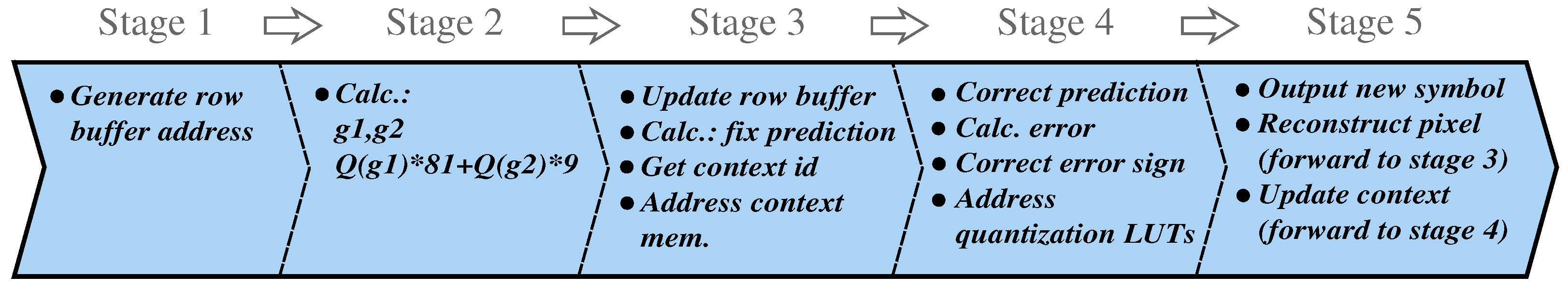
Algorithm 1 describes the pixel loop. This code structure allowed a deep pipeline (shown in Figure 3), which reads the row buffer, computes the quantized gradients $g_1$ and $g_2$, which do not depend on the previous pixel (after quantization), and starts to compute the context id before the previous pixel quantization is finished. To obtain the context id and sign, the value $Q\left(g_1\right)·81+Q\left(g_2\right)·9+Q\left(g_3\right)$ is computed, where only the $g_3$ gradient uses the previous pixel. Then, $Q\left(g_1\right)·81+Q\left(g_2\right)·9$ can be computed in an earlier stage, which is what the pipeline does. Observe that the gradients order in the equation was chosen such that the dependency between loop iterations is eased, as the component requiring $g_3$ (which cannot be computed earlier) is not multiplied by any factor.

Algorithm 1 Pixel loop algorithm structure

1: $q\_pixel\leftarrow first\_px$   2: for$i\in [1,image\_size)$do   3:     #pragma HLS PIPELINE II = 2     ▹ The lossless optimized version uses II = 1          ▹ Data stored in the row buffer does not establish dependencies   4:     #pragma HLS DEPENDENCE variable=row_buffer intra false   5:     #pragma HLS DEPENDENCE variable=row_buffer inter false   6:     $Storeq\_pixelinrowbuffer$   7:     $Readnewpixel$   8:     $Computefixedprediction,contextid,andsign$   9:     $Getcontextbiasandstatistics$ 10:     $Correctpredictionandcomputeerror$ 11:     $Performerrorquantizationandmoduloreduction$ 12:     $Sendsymbolwithmetadatatotheoutput$ 13:     $q\_pixel\leftarrow Reconstructthepixel$ 14:     $Updatecontextstatistics$ 15: end for

Additionally, to improve the performance (reducing the II), the updated context data is forwarded to previous stages when two consecutive pixels have the same context (something that happens in most cases according to [23], although this depends on the nature of the images). Originally, this optimization was done explicitly in the code and using pragmas (to inform the compiler of the false dependency), but newer versions of the HLS compiler perform this optimization automatically.

Since the HLS compiler handles the scheduling of the operations, the number of pipeline stages may change depending on the target frequency and FPGA. For the tested technologies, aiming at the maximum performance, the pixel loop operations were scheduled in five stages.

3.1.1. Obtaining the Distribution Parameter ${\widehat{\theta }}_q$

The decorrelator keeps for each context a register $S_t={\sum }_{i=0}^t{z}_i$. The register and the context counter t are then processed by the downstream module S_t Quantizer (Figure 2) to obtain the quantized distribution parameter ${\widehat{\theta }}_q$. The implemented quantization procedure is a generalization of the iterative method used in LOCO-I to obtain the k parameter of the Golomb-power-of-2 coder [34] and it is described in detail in [29]. Algorithm 2 shows the coarse-grained configuration of this quantization function.

Algorithm 2 Coarse grained $\theta$ quantization function ($Q_{\theta }$)

Require:  $S_t$ Require:  t Ensure:  ${\widehat{\theta }}_q$ 1: #pragma HLS PIPELINE 2: ${\widehat{\theta }}_q\leftarrow 0$ 3: for $i\in [1,MAX\_THETA\_ID]$ do 4:     if $\mathbf{then}(St>(t<<(i-1)\left)\right)$ 5:         ${\widehat{\theta }}_q\leftarrow i$ 6:     end if 7: end for

Although this procedure could have been done within the decorrelator, it was decided to keep it separated, to ease the scheduler job and ensure this operation extended the pipeline without affecting the pixel loop performance. This operation can be compute-intensive, but as there are no dependencies among consecutive symbols, the module can be deeply pipelined, achieving high throughput.

3.1.2. Near-Lossless Quantization and Error Reduction

To handle the quantization processes, a set of tables (the term look-up table (LUT) is usually used to refer to these tables, but here it is avoided in order not to confuse it with the FPGA resource also denominated LUT) was designed to increase the system performance, taking into account that even small FPGA have plenty of memory blocks to implement these tables. The Algorithm 3 describes the error quantization (lines 1–5), modulo reduction (lines 6–10), and re-scale (line 11) processes.

Algorithm 3 Error quantization and modulo reduction

Require:  $ϵ$                        ▹ Input error Ensure:  ${ϵ}_q$                      ▹ Output symbol Ensure:  ${ϵ}_{re}$         ▹ Re-scaled error, ysed to update context bias                     ▹ Uniform quantization   1: if $ϵ>0$ then   2:     ${ϵ}_q\leftarrow (NEAR+ϵ)/(2\ast NEAR+1)$   3: else   4:     ${ϵ}_q\leftarrow -(NEAR-ϵ)/(2\ast NEAR+1)$   5: end if             ▹ Reduction modulo $\alpha$ = f(NEAR, pixel depth)   6: if ${ϵ}_q<MIN\_ERROR$ then   7:     ${ϵ}_q\leftarrow {ϵ}_q+\alpha$   8: else if ${ϵ}_q>MAX\_ERROR$ then   9:     ${ϵ}_q-\leftarrow {ϵ}_q-\alpha$ 10: end if 11: ${ϵ}_{re}\leftarrow {ϵ}_q\ast (2\ast NEAR+1)$

As suggested in [34], the error quantization can be easily implemented using a table. However, the result after the modulo reduction logic is stored in the table, as the memory resources are reduced and it helps to speed up the context update, which is one of the logical paths that limits the maximum frequency. In addition, a second table contains the re-scaled error (${ϵ}_{re}$), to avoid the general integer multiplication logic and also to ease the sequential context dependency.

Additionally, a third table is used, in this case, to speed up the pixel reconstruction process, which is the other important logical path that could limit the maximum frequency. There are several ways to perform this, as is shown in Figure 4. To our knowledge, previous implementations of the LOCO/JPEG-LS encoder reconstruct the pixel starting from the quantized prediction error (as indicated in the ITU recommendation [16]) or from the re-scaled error (e.g., [35]). Instead, we use the value of the exact prediction error (only available on the encoder), to get the reconstructed pixel. Given a $NEAR$ value, each integer will have a quantization error, which can be pre-computed and stored in a table. Then, the exact prediction error (before the sign correction) addresses the table that provides the quantization error, and it is then added to the original value of the pixel. As it can be appreciated in Figure 4, using this method greatly simplifies the computation and eases the path. This is one of the key ideas that enabled our high-throughput implementation.

These tables could be implemented as ROMs, supporting a small set of $NEAR$ values, or implemented by RAMs, which are filled depending on the $NEAR$ value currently needed. In the presented design, the latter option was chosen, giving the system the flexibility to use any practical $NEAR$ value, using 3 tables with $2^{pixeldepth+1}$ entries each. The time required to fill these memories can be masked, as stated before. Although the uniform quantization would require general integer division, the tables are filled with simpler logic. It is easy to see that, if sweeping the error range sequentially (either increasing or decreasing by 1) and starting from zero, almost trivial logic is required to keep track of the division and remainder.

If a single clock and one edge of the clock are used, the minimum II for the system will be 2. To compute the prediction, the context memory is read (memory latency $\ge 1$), then the prediction error is obtained, which is needed to address the quantization tables (also implemented with memories with a latency $\ge 1$). The result of the quantization process is used to address the next pixel context, producing a minimum II = 2.

Within a module, Vitis HLS does not allow the designs with multiple clocks or using different clock edges. However, in this case, a great improvement is not expected from the implementation of these techniques, they will imply a much greater development time and the result will tend to be more technology-dependent (given that the FPGA fabric architecture and relative propagation times vary, affecting the pipeline tuning).

3.1.3. Decorrelator Optimized for Lossless Compression

A decorrelator optimized just for lossless compression operation was also implemented. The removal of the quantization logic, plus the logic simplification that arises from using a fixed $NEAR=0$ allows going from an II = 2 to II = 1 with approximately a 25% frequency penalty in the tested technologies. That is about a 50% throughput increase (see Section 4). In this case, this pixel loop is implemented with a 4-stage pipeline and the frequency bottleneck is established by the context update.

An interesting fact about this optimization is that going from the general decorrelator to testing on hardware, a first lossless only version took less than one hour. Such fast development was possible given that just a few lines of C++ code needed to be modified. These simple modifications led to significant changes in the scheduling of the pipeline, resulting in the stated performance, which would have been much more time-consuming using HDL languages.

3.2. TSG Coder

Figure 5 shows the block diagram of the double lane TSG coder, which allows sharing the tANS ROMs without clock cycle penalties, as double port memories are used and each lane requires one port. This module can receive the output of two independent Pixel Decorrelators and process them in parallel. In this way, it allows the compression of images in vertical tiles, which was shown to improve compression for HD and higher resolution images [29].

The system was designed in a 2-level hierarchy because, as we go downstream, the basic data elements each module processes change. The input buffer works with blocks of symbols, while the subsymbol generator works at the symbol level, the ANS coder at the subsymbol level, and the output stack with blocks of packed bits. This modularization allows easily choosing the coding technique better suited for each module. The modules shown in Figure 5 are instantiated in a dataflow region synchronized only by the input and output interfaces such that each module can run independently. In Vitis HLS, this is accomplished with the following pragma:

Figure 5. High-level block diagram of the double lane TSG coder.

Figure 5. High-level block diagram of the double lane TSG coder.

3.2.1. Stages of the TSG Coder

Input Buffers

The main function of the Input Buffer is to invert the symbol order to make the adaptive coding with ANS practical (complex methods would be required otherwise). However, to avoid the use of large memories, this module creates blocks of symbols, and the order within each block is inverted (see Figure 6). The write and read pipelined functions are instantiated in a dataflow region using a ping-pong buffer, given the required non-sequential memory accesses. However, it is noted that there is an alternative with a memory of one block, which comes at the cost of slightly more complex logic.

Subsymbol Generator

Figure 7 depicts the Subsymbol Generator and how data is transformed as it goes downstream. Its main function is to decompose z in a variable-length sequence of subsymbols $z_0,..,z_n$ which is one of the main processes of the Geometric coder.

For coding efficiency reasons, the cardinality of the symbol source modeled by the z ANS ROM varies for each distribution parameter ${\theta }_q$. Then, for a given ${\theta }_q$ tANS will model a distribution of the symbols $[0..C\left({\theta }_q\right)]$. For this reason, z needs to be represented in terms of these symbols, so it is decomposed as follows: ${\sum }_{i=0}^n{z}_i=z$, where the first subsymbol $z_0$ is equal to $mod(z,C\left({\theta }_q\right))$ and all the rest are set to $C\left({\theta }_q\right)$. In this way, to retrieve z, the decoder just needs to sum subsymbols until it finds one (first encoded, but last decoded) that is different to $C\left({\theta }_q\right)$. As $C\left({\theta }_q\right)$ is always an integer power of 2, this process is simple. Finally, if it is detected that the length of this sequence is going to be greater than a design parameter $NI$ (which determines the maximum number of geometric coder iterations) the subsymbol sequence represents an escape symbol. Following this sequence, the original z is inserted in the bitstream.

As described in [29], this process is used to reduce the cardinality tANS needs to handle, which translates into significantly lower memory requirements and higher coding efficiency while keeping simple operation.

As it decomposes z and serializes the result with y (in the coupled coders version), this module establishes the TSG coder bottleneck in terms of symbols per clock cycle (not the frequency bottleneck, i.e., contains the critical path). Due to this, it was fundamental to optimize this module to be able to output a new subsymbol every clock cycle. Pipelining the modules was not sufficient to accomplish this goal. As shown in Figure 7, the z subsymbol generation process was split into two modules, one to get the required metadata and another one to decompose the symbol. Furthermore, the Z Decompose module was not described as a loop, as one normally would specify this procedure, but instead, it was coded as a pipelined state machine, which allowed reaching the desired performance. Finally, all these modules are instantiated in a dataflow region synchronized only by the input and output interfaces.

ANS Coder

As shown in Figure 8, the ANS coder is composed of three modules. For each sub-symbol, the first one chooses the tANS table according to the symbol type ($z_i$ or y) and the distribution parameter. This table is then used to obtain the variable-length code for the sub-symbol. Thus, the module implements the Bernoulli Coder and the remaining process of the Geometric Coder. However, they can be easily split, resulting in a simpler module and the ROM memories would have weaker placement and routing constraints. The module also accepts bypass symbols, which are used to insert z after the escape symbol. After the last sub-symbol is coded, the second module inserts the last ANS state as a new code. The last module packs these codes into compact bytes.

The ANS coder can accept a new input in every clock cycle. This was accomplished by instantiating the modules in a dataflow region synchronized only by the input and output interfaces and pipelining each of them with an II=1. This II was achieved by the modularization of the process and by describing all three modules as state machines.

Output Stack

Finally, the Output Stack is in charge of reversing the order of the byte stream of each block of symbols. For this, it uses a structure similar to the one employed in the Input Buffer.

3.2.2. Increasing Coder Performance

Independent Component Coders

As mentioned before, if y and z ANS coders (Bernoulli and Geometric, resp.) are independent, the coder throughput would be increased by a $(\widehat{i}+1)/\widehat{i}$ factor. As indicated in [29], $\widehat{i}$ tends to be around 1.3 for lossless coding (the worst case). Then, applying this value will result in a 1.77 times faster coder. What is more, given that z and y coders will be decoupled and almost no additional logic is required, it is expected that the maximum frequency would be at least the one achieved for the coupled coders. To implement it, the Subsymbol Generator should not serialize z and y, the tANS coder should be split in two (each with one tANS ROM) and the bit packer should merge the two code streams.

Decreasing the Maximum Iterations Limit

In addition, the worst-case performance, as well as the maximum code extension, can be controlled using the maximum geometric coder parameter $NI$. This is particularly important for implementations with limited buffering.

4. Results

This section presents how the designs were tested as well as the achieved frequencies and resource footprints. Finally, throughput and latency analyses are provided.

4.1. Test Platform and Encoder Configurations Description

In order to conduct the hardware verification, the system depicted in Figure 9 was implemented in two different Xilinx FPGA technologies, described in

Table 1. Characteristics of target parts used in this work.

Board	FPGA	SG ${}^1$	Node	LUT	FF	BRAM	DSP	URAM
Pynq Z2	Z-7020 -1	1	28 nm	53 K	106 K	140	220	-
ZCU104	XCZU7EV -2	2	16 nm	230 K	460 K	312	1728	96

${}^1$ Speed Grade (SG). For the chosen targets, Xilinx’s speed grade ranges from 1 to 3, where 1 is the slowest. In general, we include the speed grade in the name of the device using the format: {version} -{SG}.

: Zynq 7 (cost-optimized, Artix 7 based FPGA fabric) and Zynq UltraScale+ MPSoC. For all implementations, although not optimal in terms of resources, two input and output DMAs were used to simplify the hardware, as the objective was to verify the encoders building a demonstrator, not a fully optimized system. Images were sent from the Zynq $\mathsf{\mu }$P running a Linux to the FPGA fabric using the input DMAs, which accessed the main memory and fed the encoder using an AXI4 stream interface. As the encoder generates the compressed binary, the Output DMA stores it in the main memory. The evaluation of the coding system was carried out for the configurations in

Table 2. Codec configurations used in the experiments.

						# of ANS Tables
Configuration	Rel. bpp	State Bits	B	BS	C Range	for $\mathit{\theta }$	for p
LOCO-ANS4	−0.5/−5.0	4	7	2 K	1–8	11	8
LOCO-ANS6	−1.1/−5.4	6	7	2 K	1–8	15	32
LOCO-ANS7	−1.2/−5.6	7	7	2 K	1–8	16	32

These configurations correspond to the Nt4_Stcg5_ANS4, Nt6_Stcg7_ANS6, and Nt6_Stcg8_ANS7 prototypes tested in [29]. The most relevant information is given here, but for a complete description, refer to that work. ${}^1$ Bits per pixel relative to JPEG-LS baseline for $NEAR=0$ and $NEAR=1$ (see Section 5.2.1). ${}^2$ NI: Number of Geometric coder iterations. ${}^3$ BS: Block Size. In this case, 2 K means 2048. ${}^4$ C: larger ANS table symbol.

.

4.2. Implementation Results

For the tested implementations and both technologies, the critical path of the low-frequency clock domain is, in general, in the pixel reconstruction loop for the near-lossless encoders and within the update logic of the adaptive bias correction for the lossless version.

In the case of the high-frequency clock domain, the slowest paths of these implementations tend to be in the TSG coder and the output DMA for the Zynq 7020 implementation. Within the TSG coder, the critical path is, in general, either in the tANS logic (from the tANS ROM new state data output to the tANS ROM address, the new state) or in the Z Decompose module. In the case of the Zynq MPSoC, the slowest paths tend all to be in the tANS logic.

4.3. Results Evaluation

Results are analyzed in terms of throughput and latency, which are of paramount importance for real-time image and video applications.

4.3.1. Throughput

The near-lossless decorrelator critical path is in the pixel reconstruction loop, which is the same procedure used in the standard. This fact supports that the changes introduced by LOCO-ANS in the decorrelator do not limit the system performance. In the case of the lossless decorrelator, the bias context update logic limits the frequency. This procedure is the same as in the JPEG-LS standard extension, which requires an additional conditional sign inversion compared to the baseline. This tends to worsen the critical path, but it is a minor operation compared to the complete logical path. Although it achieves a slower clock, the lossless decorrelator throughput is about 50% higher than the near-lossless decorrelator, given that it achieves an II = 1 instead of II = 2.

The presented implementations represent a wide range of trade-offs between performance, compression, and resources (also cost, considering technology dimension). All of them have the Bernoulli and Geometric coders coupled, then their mean throughput will be $clk1/2.3$ MPixels/s for photographic images, where $clk1$ refers to the clock shown in

Table 3. LOCO-ANS Encoder implementation metrics for a series of configurations and target parts.

Part	Coder Config	Clk0/1 (MHz)	LUT	FF	BRAM	DSP
Z-7020	LOCO-ANS4	79.4/180.4	4580	4992	19.5	4
Z-7020	LOCO-ANS6	81.1/182.2	4832	5160	24.0	4
Z-7020	LOCO-ANS7	79.5/167.3	5095	5240	32.0	4
XCZU7EV	LOCO-ANS4	248.3/502.2	6580	5954	19.0	4
XCZU7EV	LOCO-ANS6	246.7/442.0	6867	6027	23.5	4
XCZU7EV	LOCO-ANS7	234.1/395.1	6019	5780	33.5	4
Z-7020	LOCO-ANS4-LS	65.0/183.1	3979	4160	16.5	2
Z-7020	LOCO-ANS6-LS	64.3/186.0	4248	4298	21.0	2
Z-7020	LOCO-ANS7-LS	62.8/166.6	4572	4373	29.0	2
XCZU7EV	LOCO-ANS4-LS	188.4/500.5	4706	4949	19.0	2
XCZU7EV	LOCO-ANS6-LS	187.1/447.0	4515	4225	21.0	2
XCZU7EV	LOCO-ANS7-LS	185.2/387.5	5415	5329	31.5	2

The top half features implementations that support near-lossless compression (including lossless), and the bottom half, lossless-only compression (with -LS suffix). All the presented implementations have 2 lanes and support up to 8K wide images per lane. ${}^1$ Clk0 is the low-frequency clock used for the pixel decorrelation process, while clk1 is the high-frequency clock used for the coder. See Figure 2.

. In this way, for a given configuration and target, the TSG coder will have in the mean between 83% and 98% higher throughput than the near-lossless decorrelators for the Zynq 7020 implementations and between 47% and 76% for the Zynq MPSoC. In the case of the lossless optimized decorrelators, this performance gap is reduced to (15%, 26%) and (−10%, 16%), for Zynq 7020 and Zynq MPSoC, respectively. From the presented implementations, just one of them shows a lower TSG coder throughput. In this case, the increased compression ratio comes at the cost of not only higher memory utilization but also a throughput penalty.

However, it is observed that many possible optimizations of the TSG coder exist, and particularly of the tANS procedures. The Z ROM memory layout can be enhanced to significantly reduce the memory usage, which could have a positive impact on the maximum frequency as Table 3 suggests. Furthermore, alternative hardware tANS implementations exist [30], which may allow a wider range of performance/resources trade-offs.

The obtained results support the hypothesis that the use of the proposed TSG coder, which has a compression efficiency higher than the methods used in JPEG-LS, will not reduce the encoder throughput. This is observed in the hardware tests, where the encoder pixel rate is determined by the decorrelators when photographic images are compressed, except the lower TSG coder throughput case (LOCO-ANS7-LS in the Zynq MPSoC). As expected, this is not the case for randomly generated images, as the coder requires larger code words for them, and then, it is the TSG coder the one that limits throughput, particularly for small images and lossless compression.

4.3.2. Latency

The implemented decorrelator latency is determined by the initialization time plus the pixel loop pipeline depth, which results in $512+6=518$ cycles. For the lossless optimized version, this is reduced to $365+4=369$ cycles. In the case of the low-end device implementation (Zynq 7020), this results in 6.3 $\mathsf{\mu }$s and 5.8 $\mathsf{\mu }$s latency, respectively. As mentioned before, if required, the initialization time could be reduced or even completely masked, but these optimizations were not implemented due to compiler limitations, and the fact that it was considered that the potential benefits were low.

It is a bit more complicated to obtain the TSG coder latency, as it is data-dependent, and the coder works with blocks of symbols. To determine the marginal latency (delay added by the coder), we consider the time starting when the last symbol of the block is provided to the coder until the moment the coded block is completely out of the module. Then, avoiding the smaller pipeline delay terms, the TSG coder latency can be computed as:

$$(1+\overline{subsym\left(z\right)})·BS+\lceil bpp/out\_word\_size\rceil ·BSclockcycles$$

(5)

Here, $BS$ is the block size, $\overline{subsym\left(z\right)}$ is the mean subsymbols z is decomposed into, $bpp$ is the mean bits per pixel within the block and $out\_word\_size$ is the size (in bits) of each element of the output stack. The latency is dominated by two modules: the Subsymbol Generator (first term of the equation) and the Output Stack (second term). This is because, as mentioned before, the former creates a bottleneck given that for each input it consumes it outputs several through a single port and the latter buffers the whole block of output bytes and outputs it in the inverse order.

To obtain a pessimistic mean latency, we assume a low compression rate of 2 ($bpp=4$). The block size is set to 2048, the output stack word size to 8, and $\overline{subsym\left(z\right)}\approx \overline{i}=1.3$ (as determined in [29]). Then, for the Zynq 7020 implementation, the mean TSG coder latency is 31.9 $\mathsf{\mu }$s.

To estimate a practical upper bound to this latency, the following image compression case was analyzed:

• Image pixels equal to $BS=2048$. In this way, we maximize the block used while keeping the pixel count low, so the decorrelator’s capability to learn the statistics of the image is reduced.
• Pixels independently generated using a uniform distribution (worst-case scenario) and the errors model hurts compression (the prior knowledge is wrong).
• Image shape: 64 × 32 (cols × rows). This shape allows visiting many different contexts, and then, the adaptation of the distribution parameter $\widehat{\theta }$ will be slower, thus increasing the resulting bpp.
• $NEAR=0$ (lossless compression): which maximizes the error range and bpp.

From a set of 100 images generated in this way, we took the lower compression instance, where $bbp=9.844$ and $\overline{subsym\left(z\right)}=6.31$. This code expansion is due to the fact that the prior knowledge embedded in the algorithm (coming from the feature analysis of photographic images, such as the correlation between pixels) is wrong in this case and, as the image is small, it does not have enough samples to correct this. Moreover, given that the range of the $\theta$ distribution parameter was determined with photographic images, additional $\theta$ tables may be needed for these abnormally high entropies. Then, using the presented formulas, we obtain 97.2 $\mathsf{\mu }$s as a practical upper bound on the encoder latency for the Zynq 7020 implementation running at 180 MHz.

Although the presented system establishes a trade-off between latency and compression, the achieved latency is remarkably low and suitable for many real-time systems. Moreover, it is possible to tune this trade-off by modifying the implementation parameters.

5. Discussion

In this section, we evaluate the results presented in the previous section as well as analyze them taking prior works into consideration.

5.1. Related Work

There exists a large set of compression methods that achieve a very wide range of compression-resources-throughput trade-offs, but not all have an amenable hardware implementation. The use of dynamic structures tends to make logic slower and require a higher footprint. For example, JPEG-XL [36] can achieve better lossless compression ratios than JPEG-LS, but for that, it needs very flexible contexts and non-trivial logic is used to optimize their histograms and the rANS tables to code for these functions. Furthermore, the use of large memories, like in the case of inter-frame video compression, tends to require external memories, which also contributes significantly to the system power requirements. Given the fact that this work targets real-time and, in general, highly constrained applications with bounds on the errors generated by the compression system and considering the already mentioned features of the JPEG-LS codec that makes it very suitable for these applications, the discussion is focused on JPEG-LS-like codecs, analyzing the trade-offs within this subregion of the metrics space.

Table 4. Comparison with other codec implementations.

Implementation	Tech	PR	Rel. bpp	Lanes	Mem. Bits	Area
LOCO-ANS6	Zynq 7020 -1	40.6	−1.1/−5.4	2	442.4 K	1042 Slices + 2 DSP
LOCO-ANS6	Zynq US+ -2	123.4	−1.1/−5.4	2	433.2 K	718.5 CLB + 2 DSP
Chen et al. [19]	Virtex 6	25.8	+6.4/+13.0>	2	131.4 K	4177 Slices
LOCO-ANS6 [29]	Rasp. 3B	6.3	−1.1/−5.4	1
Fast JPEG-LS [35]	Rasp. 3B	9.2	0/0	1
LOCO-ANS6 LS	Zynq 7020 -1	64.3	−1.1/–	2	387.0 K	639 Slices + 1 DSP
LOCO-ANS6 LS	Zynq US+ -2	187.1	−1.1/–	2	387.0 K	548 CLB + 1 DSP
Daryanavard et al. [37]	Stratix 2	155	$\approx 0$/–	1	9.5 K + 1 row	573 ALUT
Murat [20]	Virtex 7 -2	207.8	0/–	1	NR	567 Slices
Kau et al. [21]	Cyclone II	113.0	+1.1>/–	1	12.8 K + 1 row	2184 LE

The top half features implementations that support near-lossless compression (including lossless), and the bottom half, lossless-only compression. Memory bits and area are normalized by the number of lanes. NR: indicates information not reported. When available, the speed grade is shown to the right of the device name with the “-{speed grade}” format. ${}^1$ PR: Pixel Rate in MPixels/s/lane. ${}^2$ Bits per pixel percentage decrease (if negative) or increase (if positive) relative to JPEG-LS baseline for $NEAR=0$ and $NEAR=1$. Data from Figure 10. Lossless-only compression implementations can only provide $NEAR=0$. ${}^3$ This work. ${}^4$ Software implementations running in Raspberry 3B, with a single thread. ${}^5$ Standard-compliant JPEG-LS implementation. ${}^6$ 12-bit image support.

shows key metrics of the most relevant hardware and, for performance comparison, software codecs implementations. In this section, to provide clearer explanations, we focus on the balanced LOCO-ANS6 configuration.

5.2. Comparison Considerations

Before diving into the analysis of the presented work in light of other works in the area, we examine what we consider the most relevant aspects of the comparison process itself that condition it.

5.2.1. Compression Trade-Offs

The fact that most of these implementations use different algorithms complicates performance comparisons, particularly because the compression ratios for a given dataset are not available. Then, it is hard to analyze the trade-offs that each design implies. Although many works claim to be standard-compliant, some present a design that it is not, as they apply several changes to the algorithms, in general, to simplify and/or speed up the implementation. Not supporting the run-mode is a common one.

In [21], for example, we note they introduced the following changes without assessing the implications:

• Not using run-mode.
• Not clamping the corrected prediction (see A.4.2 ITU-T.87). Due to this, the range of the prediction error is increased and, given that JPEG-LS uses limited-length Golomb codes, the binary code after the escape code needs to be increased by 1 bit.
• Error modulo reduction is applied after context bias update (see A.4.5 ITU-T.87).
• Not including the error sign correction required by the bias update (see A.4.3 ITU-T.87). Not applying the error sign correction will have a negative impact on compression, as it is needed to perform the context merge.
• Not limiting the maximum bias correction (see A.6.2 ITU-T.87).

To quantify the impact on the throughput of these changes, we utilize the Vitis HLS implementation feature, which instantiates the resulting HDL module in the target device, performs RTL synthesis followed by place and route (P&R). In this way, it allows obtaining a good estimation of the performance of a module in a non-congested implementation. With these changes, the tool reports that the lossless only decorrelator achieves 100 MHz in the Zynq 7020 (a 55.5% performance increase).

Of course, provided that the trade-offs are understood, changes to the algorithms that improve performance can be useful. For example, in [37] the bias update mechanism was replaced by a more precise one, which also allowed a much more feed-forward pipeline, resulting in a fasted encoder at the cost of resources. However, in this case, it is not clear whether the presented results are implementation ones or just RTL synthesis.

To better compare the encoders, we run compression experiments where, apart from LOCO-ANS and JPEG-LS, we tested JPEG-LS without run mode and JPEG-LS without run mode with 32 × 64 tilling (max tile size supported by [19]). These non-standard JPEG-LS implementations were obtained through the modification of the reference libjpeg codec [38]. Given the number of changes, and the fact that it probably has issues, we do not attempt to reproduce the algorithm implemented in [21]. In this experiment, we used the photographic (non-artificial) images of the 8-bit gray image dataset maintained by Rawzor [39] for $NEAR\in [0..3]$. The results are presented in Figure 10. As it can be appreciated, even when dealing with photographic images, the run-length coder does have a noticeable impact on compression. While LOCO-ANS6 output file size is 1.1%, 5.4%, 9.2%, and 13.4% smaller than JPEG-LS output (for $NEAR\in [0..3]$, respectively), removing the run-length coder increases it by 1.1%, 6.8%, 14.4%, and 22.3%.

Moreover, we can appreciate the effect of different tile sizes. Diving the image in 2 columns (LOCO-ANS6 (2 lanes)), which can be compressed in parallel, improves JPEG-LS by 1.4%, 5.9%, 9.9%, and 14.2% for $NEAR\in [0..3]$. We estimate that this improvement comes from the intuition that, for wide images, image statistics vary slower when scanning an image in columns, so the model is more accurate and then, higher compression is achieved. However, using small tiles, and particularly reducing the height, the encoder model does not have enough samples to learn the image statistics, so it does not make good estimations. As a result, JPEG-LS with no run mode with 64 × 32 tiles worsens compression even further, increasing the output file size by 6.4%, 13.0%, 20.3%, and 28.0%, compared to JPEG-LS.

5.2.2. Implementation Technology

Another problem is how to normalize speed, considering the target technology. In the literature, we find implementations in a wide range of devices, using different technologies. Even within the Xilinx FPGAs, it is hard to make performance comparisons as both programmable logic fabric architecture and manufacture node change. Although FPGAs have increased their maximum clock frequency with time, differences between subsequent releases vary and greater variability can exist within a release, considering different architectures and speed grades. Additionally, the clock frequency of feed-forward compute engines (without data dependencies) was able to increase much more with the introduction of more pipeline stages within FPGA hard blocks, like on-chip memories and DSPs. However, codecs with good compression ratios, and particularly JPEG-LS, have feedback loops that cannot be easily sped up.

For a subset of the Xilinx FPGAs used for the hardware codecs works,

Table 5. Example of FPGA propagation and set-up times relevant to the critical paths present in most implementations for different technologies.

FPGA Part		Info			Propagation Time			Set Up
Device	SG	Vcc *	Year	Node	LUT	FF	BRAM (no reg)	BRAM
Spartan 3	−5	1.2	2003	90 nm	530	630	2090	430
Spartan 3	−4	1.2	2003	90 nm	610	720	2400	490
Virtex 6	−1	1	2009	40 nm	90	390	2080	620
Virtex 6	−3	1	2009	40 nm	60	290	1600	470
Artix 7	−1	1	2010	28 nm	130	530	2460	570
Zynq 7020	−1	1	2011	28 nm	130	530	2460	570
Virtex 7	−2	1	2010	28 nm	50	270	1800	420
Zynq US+	−2	0.85	2015	16 nm	35–50	80	979–1020	283

Propagation and setup times values expressed in picoseconds. * Recommended or middle of range internal device voltage in Volts. ${}^1$https://www.xilinx.com/support/documentation/data_sheets/ds099.pdf, accessed on 23 October 2021. ${}^2$https://www.xilinx.com/support/documentation/data_sheets/ds152.pdf, accessed on 23 October2021. ${}^3$https://www.xilinx.com/support/documentation/data_sheets/ds181_Artix_7_Data_Sheet.pdf, accessed on 23 October 2021. ${}^4$https://www.xilinx.com/support/documentation/data_sheets/ds191-XC7Z030-XC7Z045-data-sheet.pdf, accessed on 23 October 2021. ${}^5$https://www.xilinx.com/support/documentation/data_sheets/ds183_Virtex_7_Data_Sheet.pdf, accessed on 23 October 2021. ${}^6$https://www.xilinx.com/support/documentation/data_sheets/ds925-zynq-ultrascale-plus.pdf, accessed on 23 October 2021. ${}^7$ Values obtained with the Vivado software from a subset of paths of one of the presented implementations.

shows key times involved in the context update logic, which determines the clock frequency of most of these implementations. Observe the relative magnitude of the BRAM clock to output propagation time (without output register) compared to other metrics and that it consumes a significant part of the respective clock periods. Of course, the information in this table is not enough to have an accurate model that would allow fair comparisons between technologies, among other reasons, because routing tends to be a major contributor to the critical paths in FPGA implementations and there is no clear way to compare different fabric architectures. However, this data does seem to explain, at least in part, the frequency jump from Zynq 7020 -1 to Zynq UltraScale+ -2 that we observe in Table 3.

To overcome this, Ref. [20] implemented their architecture, which seems to be standard compliant, in a set of devices used by previous works. As a result, the presented design compared favorably both in terms of speed and resources. For this reason, this work, which achieves 207.8 MPixel/s in a Virtex 7 speed grade 2 with JPEG-LS compression rate, is taken as a reference point to analyze the proposed lossless encoder results. In the near-lossless case, we compare to [19], which is the closest to standard-compliant and faster design in the literature.

5.3. Lossless-Only Encoders Comparison

The Vitis HLS implementation feature was used to estimate the clock frequency that LOCO-ANS6 would achieve in a Virtex 7 -2, used by the lossless reference architecture. Although the resulting pipeline of the lossless only decorrelator is very similar, the maximum frequency obtained after P&R is 120 MHz. The performance gap probably comes from the lower level optimizations applied to the context bias update path, as described in [40] and later improved in [20], which is the frequency bottleneck of our and their implementations.

At first glance, for lossless, LOCO-ANS6 achieves a compressed image 1.1% smaller than JPEG-LS (see Section 5.2.1), at the cost of throughput. However, the TSG coder is able to achieve 288 MHz in that device for the 6 ANS configuration. That is, 1.39 times faster than the reference design. Thus, if the Bernoulli and Geometric coder are decoupled (independent ANS states) and an optimized decorrelator is used, the TSG coder would not be the system bottleneck as, on average, it requires running 1.3 times faster.

In practice, we may find symbol sequences that increase the local mean of Geometric coder iterations, particularly with very noisy images, but this can be countered by decreasing the iterations limit (also limiting code expansion) and increasing the cardinality of the tables (decreasing mean iterations). Additionally, increasing the block size (which also improves compression) and using buffering between the decorrelator and the coder can mitigate the eventual performance throttling.

Finally, note that these positive results arise from comparing an HLS coder implementation with the best performing and carefully designed HDL decorrelator.

5.4. Near-Lossless Encoders Comparison

The reference near-lossless JPEG-LS encoder implementation does not support the run coder and has a maximum tile size of 32x64 [19]. Then, the achieved compression ratio is considerably lower than the JPEG-LS standard. The negative effect of not supporting the run-length coder increases with the $NEAR$ parameter, as lower entropy symbols are generated and the Golomb coder becomes less and less efficient as can be appreciated in Figure 10. LOCO-ANS exhibits the opposite behavior, as the TSG coder is very well suited for near-lossless compression. As a result, LOCO-ANS6 (single lane) achieves 7.0%, 16.2%, 24.5%, and 32.4% smaller output size compared to the near-lossless reference implementation. Using the two lanes in parallel to compress an image widens further this compression gap to 7.4%, 16.7%, 25.1%, and 33.0%.

Regarding performance, the reference implementation decorrelator has two lanes with an II = 2 running at 51.68 MHz (25.84 Mpixels/s/lane) in a Virtex 6-75t. These lanes share a single Golomb encoder with II = 1 running at the same frequency. This performance is surpassed by our implementation, also with two decorrelator lanes with II = 2 running at 81.1 MHz (40.55 Mpixels/s/lane for photographic images of medium and above size) in a Zynq 7020. However, this reference implementation was designed for 12-bit images, which worsens the two feedback paths that can limit the encoder performance. For this reason, to better compare these two designs, we run an implementation with Vitis HLS, configuring our decorrelator to work with 12-bit images. As the newer toolset starting from Vivado (almost 10 years old) does not support devices prior to the 7 series, the low-end Zynq 7020 (with the lowest speed grade) was targeted as opposed to the higher end Virtex 6. Table 5 gives a hint supporting that this decision favors the reference implementation as all Virtex 6 timings are noticeably smaller than the chosen target. The Virtex 6 speed grade used in that work is not reported, but this consideration is still applicable to the slowest Virtex 6 as it can be appreciated in the table. As a result, the 12-bit HLS decorrelator achieved a clock of 67.3 MHz after P&R, still a 30% higher throughput.

We attribute this performance increase to the alternative method used to reconstruct the quantized pixel (Section 3.1.2). The reference implementation uses the multiplication by inverse trick to implement the division and applies a compensation scheme to correct the errors derived from this technique while using 15 bits for the fractional part. For very deep pixels, this might be more efficient, but in the proposed architecture, using a table, we achieve a greater simplification and reduction of the critical path. For deeper pixels, larger tables would indeed be required. However, the needed type of memories are abundant (see Table 1), and for this case, targeting up to 12-bit images, only 8 36 K on-chip memories are required (in the case of Xilinx devices). The performance increase comes at the cost of memory resources, but as it can be observed comparing Table 1 and Table 3, this resource is not the limiting factor.

Again, as mentioned before, these positive results were obtained comparing an HLS implementation with carefully designed HDL ones. Additionally, as noted in Section 3, further optimizations are possible. However, for the purpose of this work, the presented module was optimal enough to analyze the LOCO-ANS encoder performance.

6. Conclusions

In this work a hardware architecture of LOCO-ANS was described, as well as implementation results presented, analyzed, and compared against prior works in the area of near-lossless real-time hardware image compression.

The presented encoder excels in near-lossless compression, achieving the fastest pixel rate so far with up to 40.5 MPixels/s/lane for a low-end Zynq 7020 device and 124.15 MPixels/s/lane for Zynq Ultrascale+ MPSOC. At the same time, a balanced configuration of the presented encoder can achieve 7.4%, 16.7%, 25.1%, and 33.0% better compression than the previous fastest JPEG-LS near-lossless implementation (for an error tolerance in $[0..3]$, respectively).

In this way, the presented encoder is able to cope with higher image resolutions or FPS than previous near-lossless encoders while achieving higher compression and keeping encoding latency below 100 $\mathsf{\mu }$s. Thus, it is a great tool for real-time video compression and, in general, for highly constrained scenarios like many remote sensing applications.

These results are in part possible thanks to a new method to perform the pixel reconstruction in the pixel decorrelator and the high-performance Two-Sided coder, based on tANS, which increases the coding efficiency. Moreover, as mentioned throughout the article, it is noted that further optimizations of the presented system are possible. Finally, experiment results support that if used with the fastest lossless optimized JPEG-LS decorrelators in the state-of-the-art, this coder will improve compression without limiting the encoder throughput.

References

1. Kiely, A.; Klimesh, M. The ICER progressive wavelet image compressor. IPN Prog. Rep. 2003, 42, 1–46. [Google Scholar]
2. Visser, S.J.; Dawood, A.S.; Williams, J.A. FPGA based satellite adaptive image compression system. J. Aerosp. Eng. 2003, 16, 129–137. [Google Scholar] [CrossRef]
3. Sushma, B. Endoscopic Wireless Capsule Compressor: A Review of the Existing Image and Video Compression Algorithms. In Sustainable Communication Networks and Application; Karuppusamy, P., Perikos, I., Shi, F., Nguyen, T.N., Eds.; Springer: Singapore, 2021; pp. 275–293. [Google Scholar]
4. Al-Shebani, Q.; Premaratne, P.; Vial, P.J.; McAndrew, D.J. The development of a clinically tested visually lossless Image compression system for capsule endoscopy. Signal Process. Image Commun. 2019, 76, 135–150. [Google Scholar] [CrossRef]
5. Turcza, P.; Duplaga, M. Low-Power Image Compression for Wireless Capsule Endoscopy. In Proceedings of the 2007 IEEE International Workshop on Imaging Systems and Techniques, Cracovia, Poland, 5 May 2007; pp. 1–4. [Google Scholar] [CrossRef]
6. Li, X.; Chen, X.; Xie, X.; Li, G.; Zhang, L.; Zhang, C.; Wang, Z. A Low Power, Fully Pipelined JPEG-LS Encoder for Lossless Image Compression. In Proceedings of the 2007 IEEE International Conference on Multimedia and Expo, Beijing, China, 2–5 July 2007; pp. 1906–1909. [Google Scholar] [CrossRef]
7. Iddan, G.; Meron, G.; Glukhovsky, A.; Swain, P. Wireless capsule endoscopy. Nature 2000, 405, 417. [Google Scholar] [CrossRef] [PubMed]
8. Lone, M.R. A high speed and memory efficient algorithm for perceptually-lossless volumetric medical image compression. J. King Saud Univ.-Comput. Inf. Sci. 2020. [Google Scholar] [CrossRef]
9. Richter, T.; Keinert, J.; Foessel, S.; Descampe, A.; Rouvroy, G.; Lorent, J.B. JPEG-XS—A High-Quality Mezzanine Image Codec for Video Over IP. SMPTE Motion Imaging J. 2018, 127, 39–49. [Google Scholar] [CrossRef]
10. New Infrared Technologies. TACHYON 16k CAMERA. Available online: https://www.niteurope.com/wp-content/uploads/2017/01/TACHYON_16k_CAMERA_NIT.pdf (accessed on 28 September 2021).
11. Nagamatsu, Y.; Sugai, F.; Okada, K.; Inaba, M. Basic Implementation of FPGA-GPU Dual SoC Hybrid Architecture for Low-Latency Multi-DOF Robot Motion Control. In Proceedings of the 2020 IEEE/RSJ International Conference on Intelligent Robots and Systems (IROS), Las Vegas, NV, USA, 24 October 2020; pp. 7255–7260. [Google Scholar] [CrossRef]
12. Saidi, H.; Turki, M.; Marrakchi, Z.; Obeid, A.; Abid, M. Implementation of Reed Solomon Encoder on Low-Latency Embedded FPGA in Flexible SoC based on ARM Processor. In Proceedings of the 2020 International Wireless Communications and Mobile Computing (IWCMC), Limassol, Cyprus, 15–19 June 2020; pp. 1347–1352. [Google Scholar] [CrossRef]
13. Zhang, X.; Wei, X.; Sang, Q.; Chen, H.; Xie, Y. An Efficient FPGA-Based Implementation for Quantized Remote Sensing Image Scene Classification Network. Electronics 2020, 9, 1344. [Google Scholar] [CrossRef]
14. Li, L.; Zhang, S.; Wu, J. Efficient Object Detection Framework and Hardware Architecture for Remote Sensing Images. Remote Sens. 2019, 11, 2376. [Google Scholar] [CrossRef] [Green Version]
15. Lee, C.A.; Gasster, S.D.; Plaza, A.; Chang, C.I.; Huang, B. Recent Developments in High Performance Computing for Remote Sensing: A Review. IEEE J. Sel. Top. Appl. Earth Obs. Remote Sens. 2011, 4, 508–527. [Google Scholar] [CrossRef]
16. International Telecommunication Union. Information technology—Lossless and near-lossless compression of continuous-tone still images: Baseline (ITU-T T. 87—ISO/IEC 14495-1). ITU-T Recommendation T.87. 1998. [Google Scholar]
17. Yang, M.; Bourbakis, N. An overview of lossless digital image compression techniques. In Proceedings of the 48th Midwest Symposium on Circuits and Systems, Covington, KY, USA, 7–10 August 2005; Volume 2, pp. 1099–1102. [Google Scholar] [CrossRef]
18. Weinberger, M.J.; Seroussi, G.; Sapiro, G. From LOCO-I to the JPEG-LS standard. In Proceedings of the 1999 International Conference on Image Processing (Cat. 99CH36348), Kobe, Japan, 24–28 October 1999; Volume 4, pp. 68–72. [Google Scholar] [CrossRef]
19. Chen, L.; Yan, L.; Sang, H.; Zhang, T. High-Throughput Architecture for Both Lossless and Near-lossless Compression Modes of LOCO-I Algorithm. IEEE Trans. Circuits Syst. Video Technol. 2019, 29, 3754–3764. [Google Scholar] [CrossRef]
20. Murat, Y. Key Architectural Optimizations for Hardware Efficient JPEG-LS Encoder. In Proceedings of the 2018 IFIP/IEEE International Conference on Very Large Scale Integration (VLSI-SoC), Verona, Italy, 8–10 October 2018; pp. 243–248. [Google Scholar] [CrossRef]
21. Kau, L.; Lin, S. High performance architecture for the encoder of JPEG-LS on SOPC platform. In Proceedings of the SiPS 2013, Taipei, Taiwan, 16–18 October 2013; pp. 141–146. [Google Scholar] [CrossRef]
22. Merlino, P.; Abramo, A. A Fully Pipelined Architecture for the LOCO-I Compression Algorithm. IEEE Trans. Very Large Scale Integr. Syst. 2009, 17, 967–971. [Google Scholar] [CrossRef]
23. Ferretti, M.; Boffadossi, M. A parallel pipelined implementation of LOCO-I for JPEG-LS. In Proceedings of the 17th International Conference on Pattern Recognition, ICPR 2004, Cambridge, UK, 26 August 2004. [Google Scholar] [CrossRef]
24. Klimesh, M.; Stanton, V.; Watola, D. Hardware implementation of a lossless image compression algorithm using a field programmable gate array. Mars (Pathfinder) 2001, 4, 5–72. [Google Scholar]
25. International Telecommunication Union. Information technology-Lossless and near-lossless compression of continuous-tone still images: Extensions (ITU-T T. 870—ISO/IEC 14495-21). ITU-T Recommendation T.870. 2003. [Google Scholar]
26. Duda, J. Asymmetric Numeral Systems. arXiv 2009, arXiv:0902.0271. [Google Scholar]
27. Duda, J. Asymmetric Numeral Systems: Entropy Coding Combining Speed of Huffman Coding with Compression Rate of Arithmetic Coding. arXiv 2009, arXiv:1311.2540. [Google Scholar]
28. Duda, J.; Tahboub, K.; Gadgil, N.J.; Delp, E.J. The use of asymmetric numeral systems as an accurate replacement for Huffman coding. In Proceedings of the 2015 Picture Coding Symposium (PCS), Cairns, QLD, Australia, 31 May–3 June 201; pp. 65–69.
29. Alonso, T.; Sutter, G.; López de Vergara, J.E. LOCO-ANS: An Optimization of JPEG-LS Using an Efficient and Low-Complexity Coder Based on ANS. IEEE Access 2021, 9, 106606–106626. [Google Scholar] [CrossRef]
30. Najmabadi, S.M.; Wang, Z.; Baroud, Y.; Simon, S. High throughput hardware architectures for asymmetric numeral systems entropy coding. In Proceedings of the 2015 9th International Symposium on Image and Signal Processing and Analysis (ISPA), Zagreb, Croatia, 7–9 September 2015; pp. 256–259. [Google Scholar]
31. Najmabadi, S.M.; Tungal, H.S.; Tran, T.; Simon, S. Hardware-based architecture for asymmetric numeral systems entropy decoder. In Proceedings of the 2017 Conference on Design and Architectures for Signal and Image Processing (DASIP), Dresden, Germany, 27–29 September 2017; pp. 1–6. [Google Scholar] [CrossRef]
32. Merhav, N.; Seroussi, G.; Weinberger, M.J. Coding of sources with two-sided geometric distributions and unknown parameters. IEEE Trans. Inf. Theory 2000, 46, 229–236. [Google Scholar] [CrossRef]
33. Forconesi, M.; Sutter, G.; Lopez-Buedo, S.; López de Vergara, J.E.; Aracil, J. Bridging the gap between hardware and software open source network developments. IEEE Netw. 2014, 28, 13–19. [Google Scholar] [CrossRef]
34. Weinberger, M.J.; Seroussi, G.; Sapiro, G. The LOCO-I lossless image compression algorithm: Principles and standardization into JPEG-LS. IEEE Trans. Image Process 2000, 9, 1309–1324. [Google Scholar] [CrossRef] [PubMed] [Green Version]
35. CharLS Implementation of JPEG-LS. Available online: https://github.com/team-charls/charls (accessed on 15 June 2021).
36. Rhatushnyak, A.; Wassenberg, J.; Sneyers, J.; Alakuijala, J.; Vandevenne, L.; Versari, L.; Obryk, R.; Szabadka, Z.; Kliuchnikov, E.; Comsa, I.M.; et al. Committee Draft of JPEG XL Image Coding System. arXiv 2019, arXiv:eess.IV/1908.03565. [Google Scholar]
37. Daryanavard, H.; Abbasi, O.; Talebi, R. FPGA implementation of JPEG-LS compression algorithm for real time applications. In Proceedings of the 2011 19th Iranian Conference on Electrical Engineering, Tehran, Iran, 17–19 May 2011; pp. 1–4. [Google Scholar]
38. libjpeg. Available online: https://github.com/thorfdbg/libjpeg (accessed on 23 October 2021).
39. Rawzor Test Image. Available online: http://imagecompression.info/test_images/ (accessed on 23 October 2021).
40. Mert, Y.M. FPGA-based JPEG-LS encoder for onboard real-time lossless image compression. In Proceedings of the Satellite data Compression, Communications, and Processing XI. International Society for Optics and Photonics, Baltimore, MD, USA, 20–24 April 2015; Volume 9501, p. 950106. [Google Scholar]
Figure 1. LOCO-ANS block diagram. Source adapted from [29].
Electronics 10 02934 g001
Figure 2. LOCO-ANS hardware high-level block diagram. In blue, modules running at the lower frequency, and in red, modules running at the higher frequency.
Electronics 10 02934 g002
Figure 3. Pixel decorrelator pipeline.
Electronics 10 02934 g003
Figure 4. Quantization processes. The operations performed by tables are indicated with red ellipses.
Electronics 10 02934 g004
Figure 6. Input Buffer block diagram, showing its operation for block size N.
Electronics 10 02934 g006
Figure 7. Subsymbol Generator block diagram and data transformations within it.
Electronics 10 02934 g007
Figure 8. ANS coder block diagram showing the transformation of sub-symbols into packed bytes.
Electronics 10 02934 g008
Figure 9. Block diagram of the accelerator, μ P, and interfaces.
Electronics 10 02934 g009
Figure 10. Mean bits per pixel (bpp) obtained by JPEG-LS, JPEG-LS without run mode and LOCO-ANS.
Electronics 10 02934 g010