Abstract
The orbital characteristics of low Earth orbit (LEO) satellite systems prevent continuous monitoring because ground access time is limited. For this reason, the development of simulators for predicting satellite states for the entire orbit is required. Power-related prediction is one of the important LEO satellite simulations because it is directly related to the lifespan and mission of the satellite. Accurate predictions of the charge and discharge current of a power system’s battery are essential for fault management design, mission design, and expansion of LEO satellites. However, it is difficult to accurately predict the battery power demand and charging of LEO satellites because they have nonlinear characteristics that depend on the satellite’s attitude, season, orbit, mission, and operating period. Therefore, this paper proposes a novel battery charge and discharge current prediction technique using the bidirectional long short-term memory (Bi-LSTM) model for the development of a LEO satellite power simulator. The prediction performance is demonstrated by applying the proposed technique to the KOM-SAT-3A and KOMSAT-5 satellites operating in real orbits. As a result, the prediction accuracy of the proposed Bi-LSTM shows root mean square error (RMSE) within 2.3 A, and the prediction error well outperforms the most recent the probability-based SARIMA model.
1. Introduction
Monitoring the status of LEO satellites is limited because of limited ground access time due to the non-contact duration in orbit. Therefore, for optimal mission design and mission expansion, simulators are required to predict the satellite operation. Satellite simulators require the development and verification of each sub-system, such as attitude, power, S/W, and thermal control. Power system simulators are critical because the power system is responsible for generating, distributing, and storing energy for the operation of the satellite, and it is closely related to the mission design, satellite lifespan, and fault management [1,2].
The battery is one of the main electronic components related to the lifespan of the satellite and error management. In general, mission and error management designs must ensure that the batteries used for LEO satellites are in the operating range that guarantees expected performance of the satellite [3,4]. However, because LEO satellites have limited communication with ground stations, it is necessary to predict the power state, including the non-contact duration. Such state prediction varies depending on the operating period, season, attitude, and mission of the satellite [5,6,7], which makes its mathematical modeling difficult.
In previous studies, design and power analysis were performed in terms of the power budget [8]. That is, the power that can be generated is analyzed assuming the eclipse duration, sun irradiance, temperature, and angle with the sun in the worst condition. The power consumption is calculated by combining the average duty (or maximum values of each load of the satellite bus) and the payload. Accordingly, the power consumption combination composes a table for each mission condition and operation mode of the satellite. Then, the generated power and the consumed power are compared over the time, which is required to predict the state or current of the satellite battery [9]. However, in this analysis of the generated power, the operating period, attitude, and temperature conditions may be different from the assumptions, so that it may show a significant difference from the actual data from the orbit. Moreover, in the case of power consumption, except for some loads operating at a constant duty, the generation time and consumption values of general loads, such as actuators and heaters, are different from the assumed combinations. Thus, the estimated value can be very different from the actual data. Since the power generated and power consumed continuously vary depending on the satellite operation period and the given method, it is difficult to use the analysis developed for the existing power budget to determine the current to analyze the battery state. In addition, the inability to accurately predict the operation of the power system and battery may prevent a precise analysis when a task change or an operation analysis is required for the changes in the operating environment [10,11,12,13].
Another approach in previous studies is the time series prediction analysis method, for example, a stochastic estimation method using ARIMA or SARIMA for ground applications [14,15]. This probability-based analysis of the satellite system can be more accurate than the power-budget-based analysis, however, it is impossible to actively estimate the change in the mission and the attitude change of the low-orbit satellite system. Therefore, it may not be utilized when mission expansion and operation change are necessary, which is same to the power budget-based analysis.
Therefore, in this study, a Bi-LSTM deep neural network is proposed to predict the charging and discharging current of the satellite battery. The proposed technique is based on the optimal Bi-LSTM selection and input/output design to respond to mission changes. The proposed technique is applied to the KOMPSAT-3A and KOMPSAT-5 LEO satellites to compare and analyze the on-orbit measurement data and prediction results. The superior performance of the data-based learning applied in this study is demonstrated by comparing with the SARIMA.
The contribution of this paper is summarized as follows:
- We propose a Bi-LSTM-based network to reliably predict battery charge and discharge currents in the non-contact duration of low-orbit satellites.
- The proposed technique is one of the first techniques that can produce an accurate prediction, even in the presence of task change and expansion.
- To demonstrate the prediction performance, we apply the proposed technique to the KOMPSAT-3A and 5 satellites with different environmental conditions such as mission power, period, and orbit.
This paper is organized as follows. Section 2 discusses about how the KOMPSAT-3A and KOMPSAT-5 LEO satellites and the algorithms are used in this study, and describes the structure of the data-learning Bi-LSTM used to predict the battery charge/discharge current. It also describes the probabilistic-based SARIMA used as the comparison method. Section 3 shows how the power system and other characteristics of KOMPSAT-3A and KOMPSAT-5 satellites affect the signal processing used in the simulations. These include the characteristic orbital data, denoising preprocessing requirements, the parameters of the SARIMA model, and the selection methods for the network and hyper-parameters of bi-LSTM. Section 4 analyzes the prediction results of the LEO satellite’s charge/discharge current and compares orbit data, the operating period, and the mission performance errors based on the learned results using RMSE, MAPE, correlation coefficient, and performance analysis indicators. Finally, Section 5 draws the conclusion of the paper.
2. Background on the KOPPSAT3A and 5 Satellite Power Systems and Methods
2.1. KOMPSAT-3A and KOMPSAT-5 Electronics Power Systems
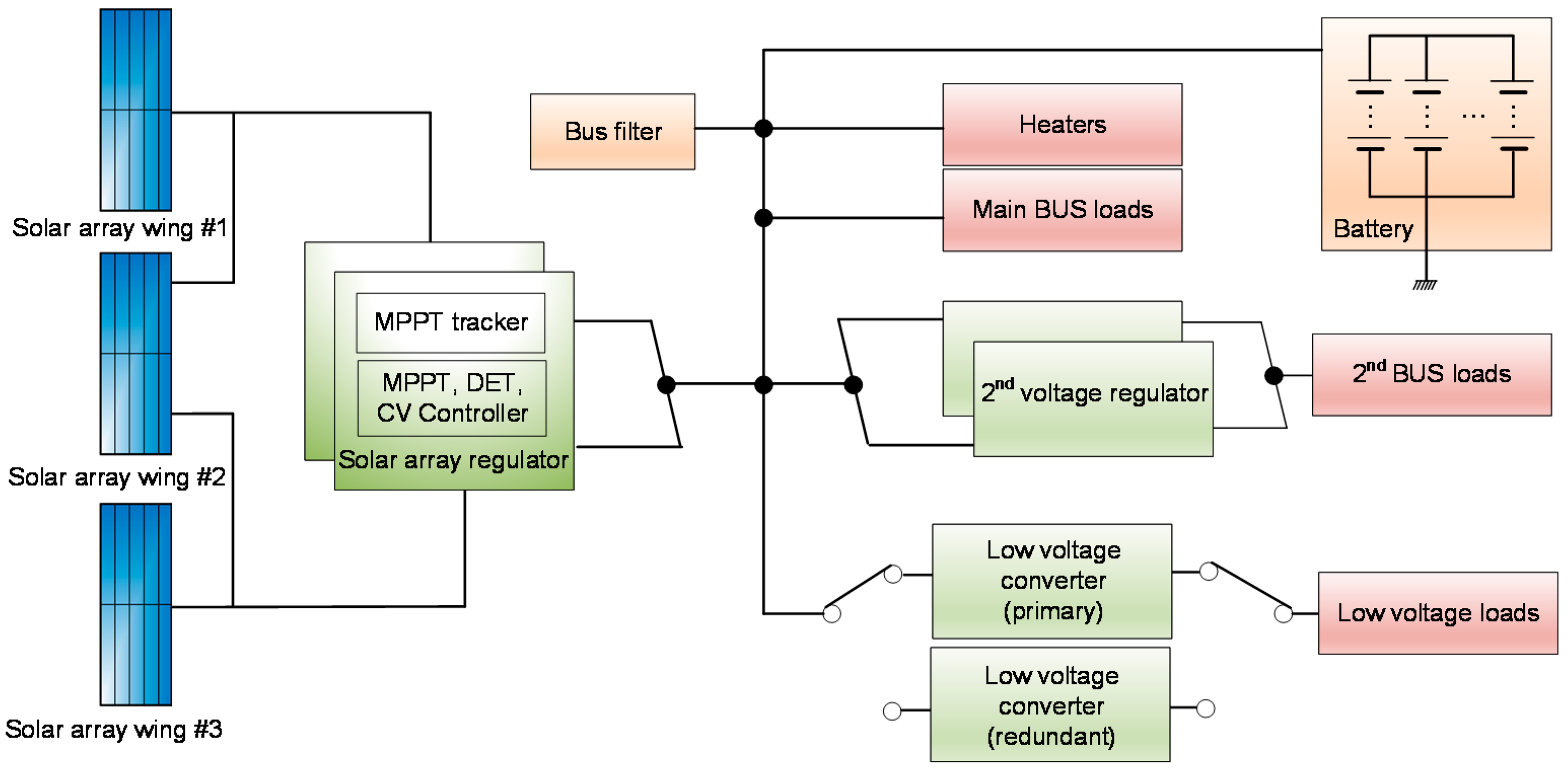
KOMPSAT-3A is an Earth observation satellite equipped with an electro-optical camera with a resolution of 55 cm and an infrared sensor that was launched on 25 March 2015. KOMPSAT-5 is also an Earth observation satellite that is equipped with a synthetic aperture radar for all-weather observation. It was launched on 22 August 2013. The power systems of KOMPSAT-3A and KOMPSAT-5 are mainly composed of four parts. They consist of a transmission system that supplies power to each load, a solar array responsible for generating the power of the satellite, a power conversion device that converts the generated power according to the load, and the battery system used during the occurrence of a load exceeding the satellite’s generated power and eclipse duration. The power system of KOMPSAT-3A is shown in Figure 1.

Figure 1.
KOMPSAT-3A electrical power system structure.
First, the solar array PV system changes the generated power according to the temperature and sun irradiance. In addition, as the short-circuit current and the open-circuit voltage change with temperature, the maximum power point changes accordingly [16]. Therefore, the PV system of each satellite must be designed according to the orbit, temperature, and power load. The KOMPSAT-3A satellite consists of three solar wings. Each wing is connected in parallel with 19 strings, and each string has 31 cells connected in series. The minimum efficiency for each cell is 27.5%. Moreover, the generated power is designed to be 1726 W or more at 28 °C based on BOL.
On the other hand, the KOMPSAT-5 satellite has two wings, and each wing has 29 strings connected in parallel. One string is designed with 31 cells connected in series. Accordingly, the minimum generated power is designed to be 1740 W or more at 28 °C based on BOL.
The power generated from the solar array is converted to primary power using a SAR. The design includes a maximum power tracking mode for maximum power production of the solar array, a constant voltage mode to prevent overcharging of the battery, and the direct energy transfer mode to prevent damage to the converter by excessive power production of the solar array. The primary converted voltage output is used for loads that include their own power conversion and loads with a wide input voltage range. However, the output voltage of the SAR is converted according to the SOC of the battery, power generation, and load. Therefore, a secondary power conversion device is included in order to supply a voltage suitable for a load whose input voltage range is specified or that does not include its own power conversion device. The secondary power conversion consists of a low-voltage converter and the regulated converter. The low-voltage converter supplies 5 V, +15 V, and −15 V power, and the regulated converter supplies a 28 V load.
Next, the battery is designed to have a charge and discharge balance based on one day in order to respond to a load exceeding the power generated during the eclipse duration and mission performance. The charging and discharging current of the KOMPSAT-3A,5 battery system is not directly controlled using a converter. The charging current of the battery is determined according to the SOC of the battery, solar array temperature, sun orientation angle, MPPT algorithm, and load. In addition, the discharge current of the battery is indirectly controlled according to the expression section based on the orbit of the satellite, the change in the load in accordance with the mission performance, and the amount of power generated according to the satellite attitude. Therefore, charge and discharge current prediction is essential for mission feasibility analysis, fault management design, and satellite simulator development.
The methods and results for predicting battery current and voltage in orbit are analyzed in order to examine the possibility of applying this prediction method proposed in this study to various satellites, using the two KOMPSAT-3A and KOMPSAT-5 satellites with different load characteristics during the mission orbit and mission performance.
2.2. Bi-LSTM Modeling
The LSTM model solves the vanishing gradient problem and long-term dependencies that occur as the sequence increases in the RNN. That is, the LSTM model can be memorized for a long period of time through memory extension, and read, write, and delete functions are performed to overcome the disadvantages of RNN [17,18,19]. The memory of such an LSTM is defined as a gate cell and is responsible for the preservation or deletion of information. Therefore, in the case of important information, it is possible to preserve it for a long duration, and the weight value for preservation or deletion is determined through the training process [20].
In general, the LSTM model consists of a forget gate, input gate, and output gate. The forget gate layer is the process of selecting information retention and removal, the input gate adds new information to the memory, and the output gate controls the value contributing to the output. The forget gate removes information from the memory using the values of previous hidden state and input, and it outputs 0 or 1 using the sigmoid function. In the case of 1, information is preserved; in the case of 0, information is deleted, and it is calculated as
where is the forget gate, σ is the sigmoid function, represents the weight matrices, is the previous hidden state, is the input, and is a constant bias value.
Next, the input gate layer () determines whether new information is added to the LSTM memory and is generally composed of a sigmoid layer and a tanh layer. The sigmoid layer receives the input and the previous hidden state, and determines the updated value. It is expressed as
where is the input gate, and is a constant bias value.
Next, the network is updated using the forget gate layer, input gate layer, tanh layer, and cell state before t − 1 is calculated in the above process. That is, a new candidate value is created to be added to the LSTM memory, and whether the existing value is maintained is expressed as a product of the forget gate. The formula for the updated cell state is expressed as:
where is the updated cell state, is the previous cell state, represents the weight matrices, and is a constant bias value.
Finally, in the output gate, the part contributing to the output is determined by Equations (4) to (5).
where is the output value, represents the weight matrices, is a constant bias value, and is the updated hidden state.
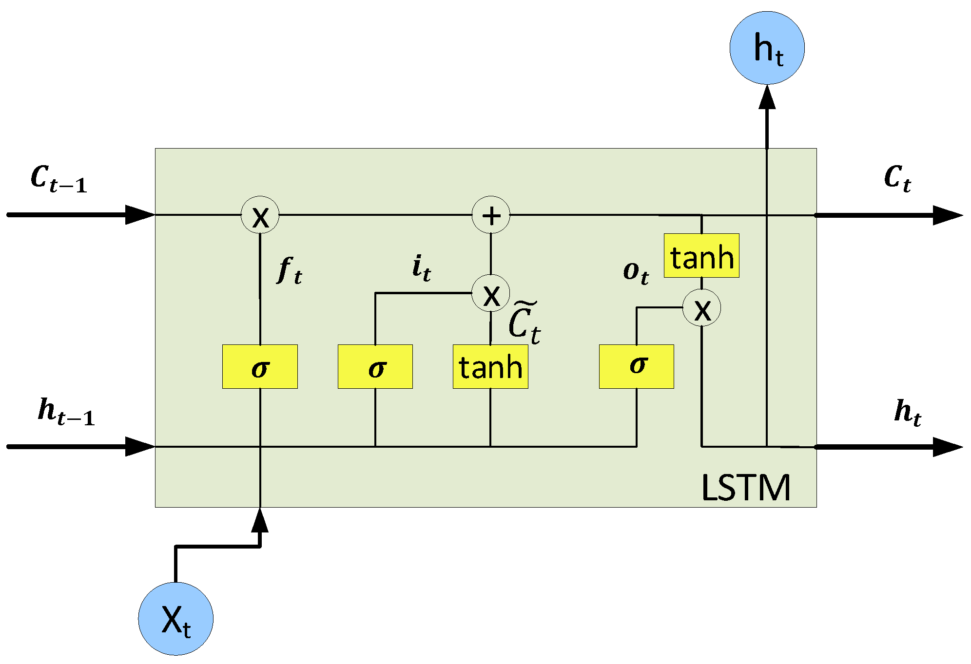
The overall concept of one LSTM model is shown in Figure 2. Bi-LSTM is a model that extends the LSTM model and learns input data from two LSTM models in the forward and backward directions. It is known that this application of LSTM twice has the effect of reducing long-term dependency and improving performance. In particular, it shows more accuracy for cases when a pattern in the reverse direction is meaningful, i.e., where the next time value affects the previous time value [18,19]. The patterns of the LEO satellite are also meaningful in the forward and reverse patterns in the battery charge and discharge profile according to the attitude, orbit, mission, etc. Therefore, Bi-LSTM was used to construct the network owing to its improved estimation accuracy.
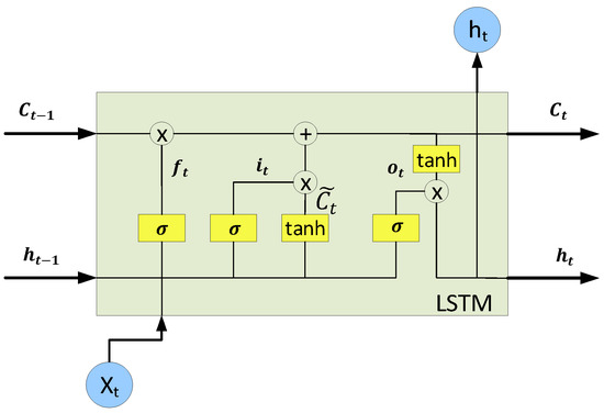
Figure 2.
LSTM structure.
2.3. SARIMA Modeling
We compare the prediction performance of the proposed Bi-LSTM model to the probability-based SARIMA model, which is widely used for power demand prediction. The ARIMA model considers the probability structure of observational values over time, including both an AR model and an MA model [21]. The ARIMA model has an auto regression order p, a difference order d, and a moving average order q. It has the advantage of deriving a model from past observations and error terms alone and is suitable for short-term prediction because it assigns greater weight to observations close to the most recent time point. However, the ARIMA model cannot consider the seasonality or periodicity of time series data. Accordingly, the SARIMA model is a forecasting technique that complements the ARIMA model. The SARIMA model can overcome these limitations by adding the SAR and SMA terms to the existing ARIMA model [21,22]. The time series has a seasonal period s, non-seasonal and seasonal autoregressive orders (), non-seasonal and seasonal differential coefficients (), and non-seasonal and seasonal moving deviation orders (). When (p,d,q)(P,D,Q)s is followed, the model is expressed as Equations (6)–(10) [23]:
where B is the backshift operator, and is independent and identically distributed
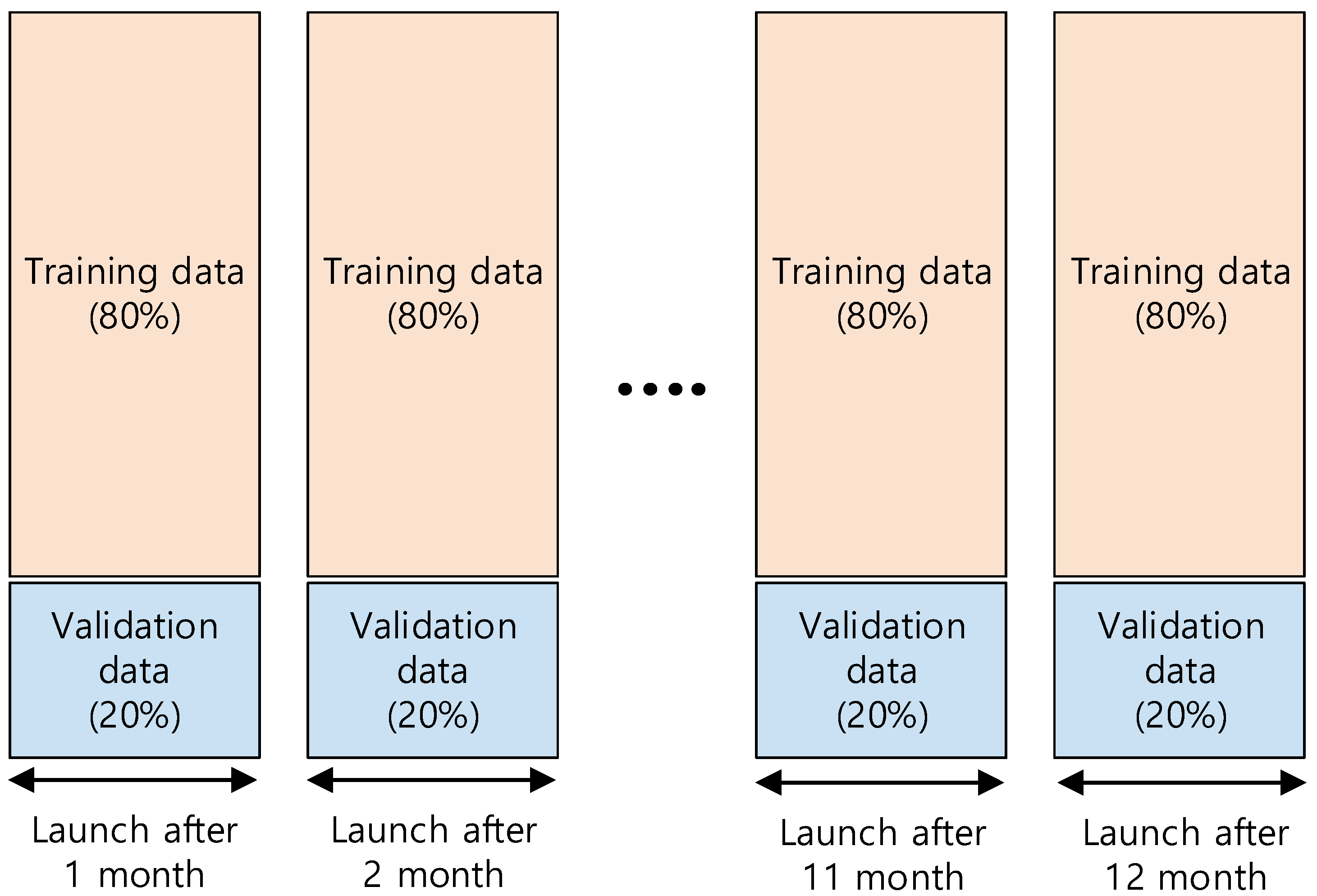
For the SARIMA model, 80% of the monthly battery current data in the dataset are used as the training dataset until one year after the launch. The remaining 20% are used as a validation dataset for parameter selection. Figure 3 shows the dataset used for training and parameter selection. In addition, for the comparison with the data-based learning results, the value that minimizes the implementation complexity and the BIC of the validation dataset is selected through the trial-and-error process and used in KOMPSAT-3A and KOMPSAT-5. The resulting values are (2,1,1)(2,1,3)12 and (2,1,2)(2,1,1)12, respectively.
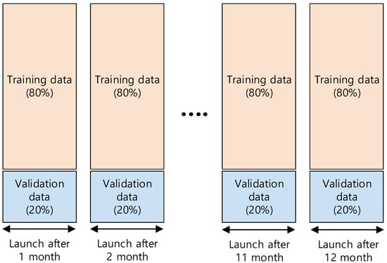
Figure 3.
Dataset for SARIMA model training for battery current.
3. Proposed Method
Because the battery-related profile of a LEO satellite has a nonlinear characteristic that depends on the SOC of the battery, the solar array temperature, the attitude of the satellite, the orbit position, the satellite bus and payload temperature, and the degradation effect of each unit, mathematical modeling has limitations. Therefore, it is necessary to consider data-based modeling methods [24,25,26], for which a preprocessing stage is required to prevent overfitting and to optimize the learning time. In the case of LEO satellite data, preprocessing is required because the data are of various types and multiple periods. In addition, for a successful data-based learning, it is necessary to select input features, a network configuration, and a parameter selection method related to the prediction output. In this section, the proposed Bi-LSTM learning model configuration, the satellite data specificity, the process for each step (including preprocessing), and the parameter selection for learning are described.
3.1. Features and Bi-LSTM Network
The features used for estimating the current profile of the LEO satellites are the sat-elite’s orbital position, attitude quaternion, mission mode of the satellite, eclipse state, week and date information for one year, the week information after launch, and the solar array angle. These features are closely related to the battery charging/discharging current and correspond to values that can be accurately predicted on the ground or determined through mission design.
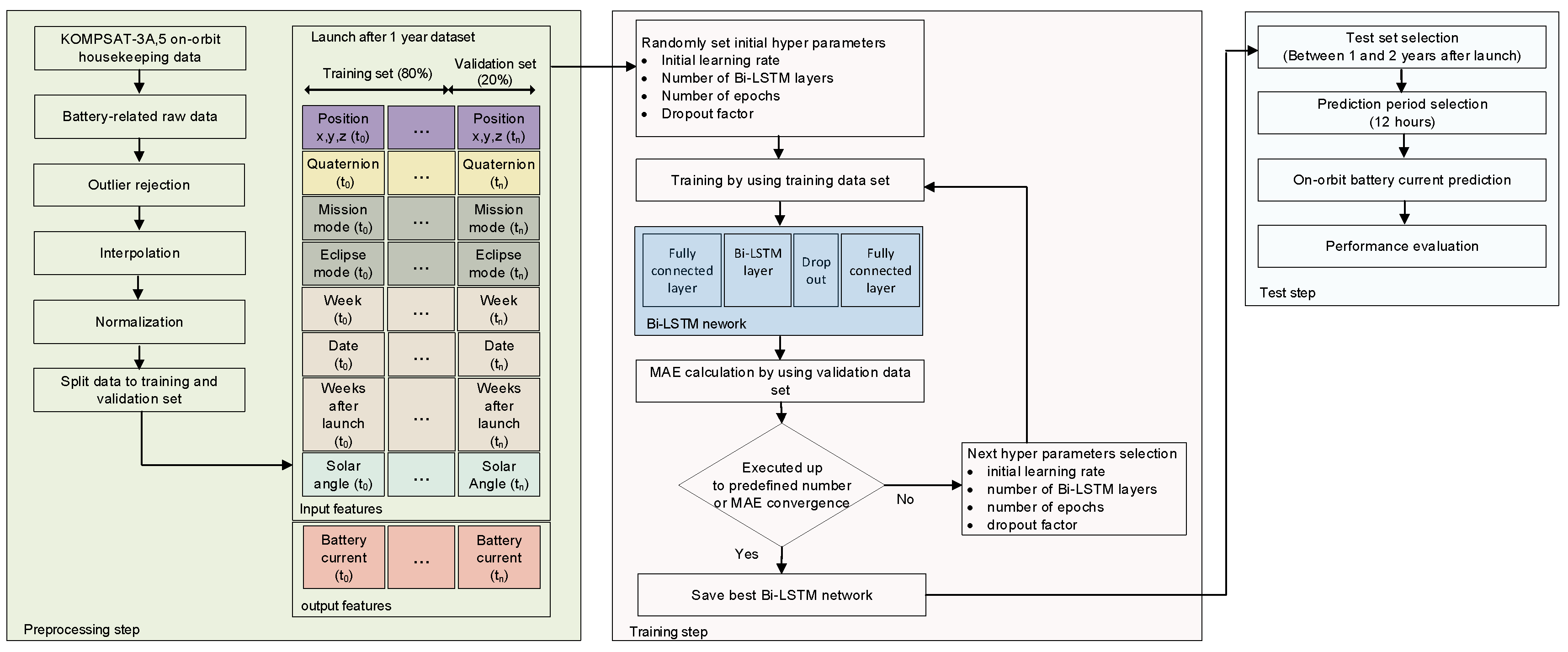
Figure 4 shows the framework for Bi-LSTM-based battery current prediction. The whole process for prediction is carried out in three steps. First, preprocessing is per-formed to prepare the data for learning. For the preprocessing process, the raw data of both of the features for prediction and battery current among the house keeping data of two years after launch are collected for each satellite. Afterwards, outlier rejection, interpolation, and normalization processes are performed to suit the characteristics of the satellite’s raw data. Each preprocessed feature is divided into training and validation sets for learning and optimization. Additionally, a test set for performance evaluation is selected. In this paper, similarly to the SARIMA, 80% of the data for one year after launch are classified as a training set and 20% as a validation set. In addition, data from one to two years after launch are used as the test set.
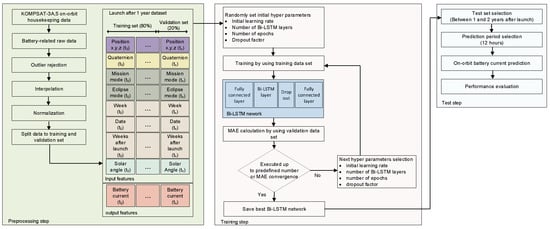
Figure 4.
Proposed framework of battery current prediction.
Next, a learning process for Bi-LSTM model selection is performed. The Bi-LSTM network consists of a fully connected layer, a Bi-LSTM layer, a dropout layer, and a fully connected layer. The Bi-LSTM layer is selected because the data of the battery current of the low-orbit satellite are meaningful in that both forward and backward time series have a causal relationship in the prediction. In addition, a dropout layer is added to prevent overfitting. In addition, since the battery current is predicted using multiple inputs, the fully connected layer is used for the input and output. As parameters for the Bi-LSTM network model, the initial learning rate, bi-layer number, training epoch, and dropout factor are selected. After that, training is performed using each randomly selected initial value, and the MAE, a cost function, is calculated using the validation dataset. Next, by using Bayesian optimization, the next model parameter is selected and learning is repeated until the cost function converges or reaches a specified number of times. The Bi-LSTM network model is selected using the parameters chosen through this process. Finally, performance evaluation is performed using the selected test dataset. When evaluating the performance, the prediction period is selected by considering the contact period of the ground station of KOMPSAT-3A and 5. In this paper, 12 h is selected by assuming the worst condition of the contact period with the ground.
Figure 5 shows the battery prediction technique proposed in this study. Pretraining is performed using preprocessed features. Prediction is performed using the best Bi-LSTM network selected through the process in Figure 4. The input features for predicting the battery current are factors that are predictable or designed on the ground, and normalization is performed to input them into the learning model. Then, the processed input features are input into the pretrained model to verify the output value. Finally, the features selected as input/output in this paper undergo a process to restore the predicted battery current value while going through the normalization process.
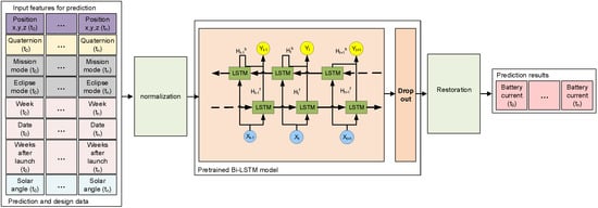
Figure 5.
Proposed on-orbit battery current prediction based on Bi-LSTM network.
3.2. Preprocessing for Bi-LSTM Network Training
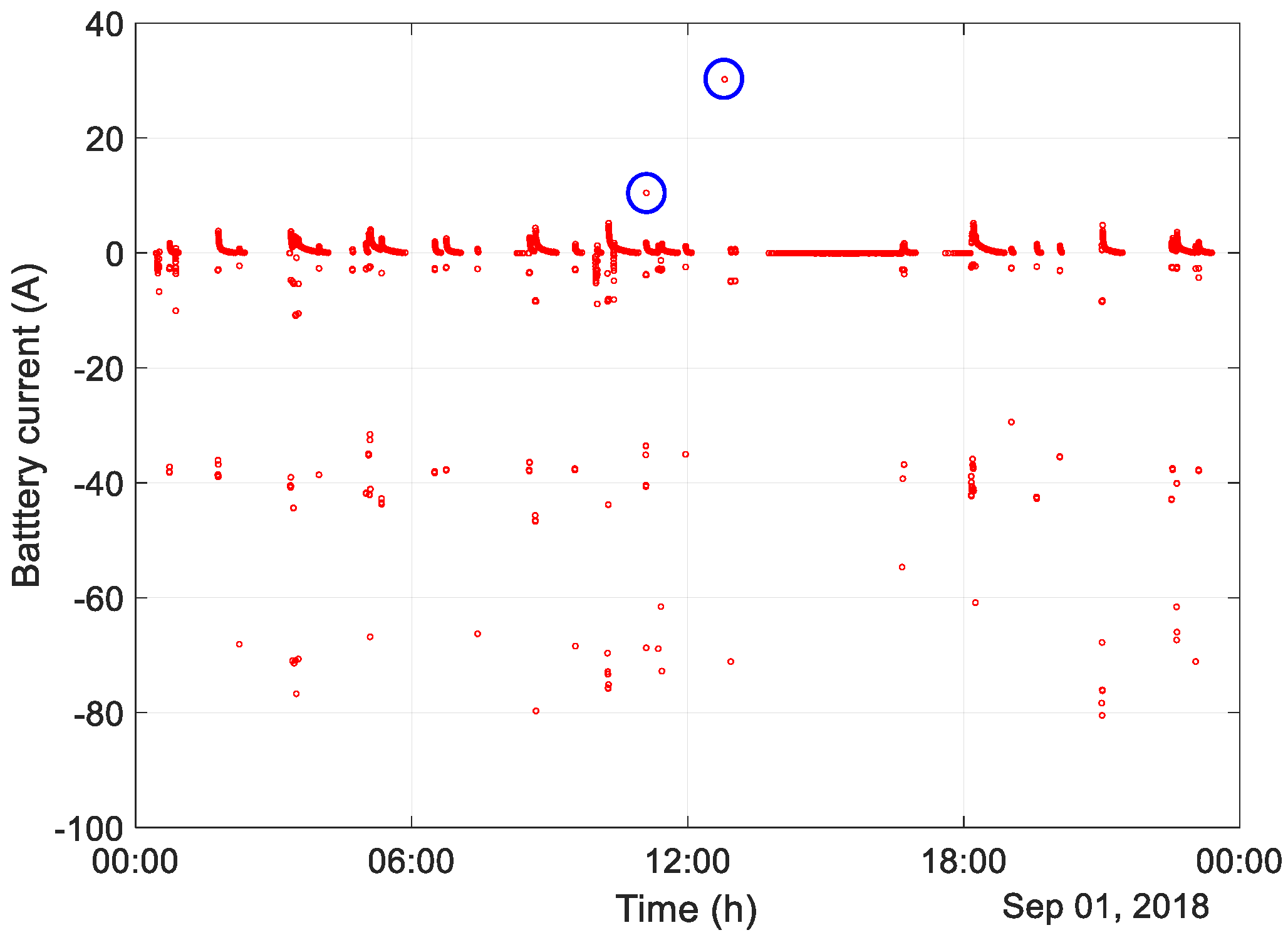
Satellites operate in harsh environments with radiation compared to the ground. Therefore, a SEU may occur on account of these radiation conditions, and instantaneous noise may occur when satellite data is stored and transmitted. Therefore, noise occurs independently of the physical correlation, as shown by the values in the blue circles in Figure 6. The noise must be removed because it can damage the accuracy of the learning model. In this study, the IQR method is used to remove outliers, as shown in Equations (11) and (12). The IQR is a powerful method for detecting outliers in data. It arranges the data in ascending order and divides them into quadrants to determine the normal range. The IQR refers to the value obtained by subtracting the 25% quartile from the value of the 75% quartile and by assigning a weight to this value. The low and high limits are set as in Equations (11) and (12), and the data between these values are estimated to be normal. Generally, a weight of 1.5 is used for the IQR. However, when this is used for the KOMPSAT satellite, some normal data are judged as outliers. Therefore, because the frequency of occurrence of KOMPSAT-3A and 5 satellites data noise is low, it is necessary to select a weight other than 1.5. In this paper, while changing the weight of the IQR from 1.5 to 3 in the raw data of the satellite, 2.5, which was a value from which outliers were appropriately removed, is selected as shown in Equations (11) and (12).
where Q1 and Q3 are the 25% and 75% quartiles, respectively.
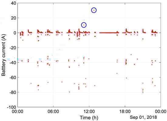
Figure 6.
KOMPSAT-5 housekeeping data noise.
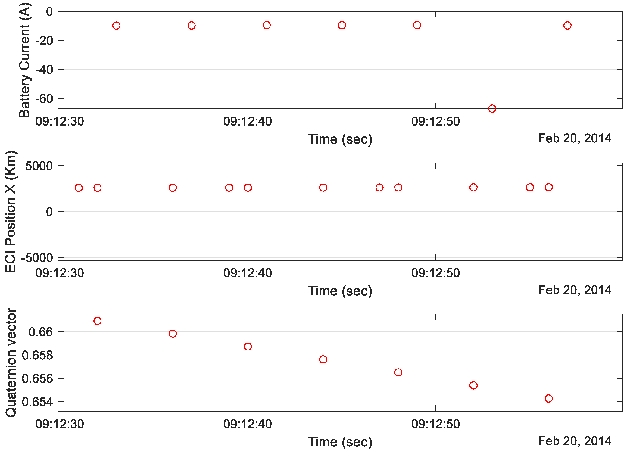
Because of the limited access time with the ground station, the LEO satellite transmits housekeeping data over several cycles within the downlink budget. Therefore, the gap time of housekeeping data and the time at which they are saved are also different, as shown in Figure 7. In addition, an empty information section is created when outliers are removed.
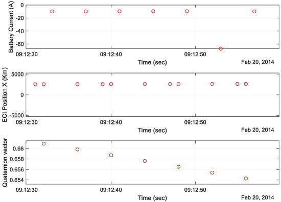
Figure 7.
KOMPSAT-5 on-orbit current, position, and attitude data.
Therefore, to use different period information and empty sections for learning, synchronization through interpolation of these data is required. In this study, synchronization is performed by conducting a linear-based interpolation [27,28].
There are various types of data for the satellite features that are used for training, as shown in Figure 7. That is, data of various scales and ranges, such as trajectory, attitude, and current, are used. It also contains categorical data such as mission mode. An example of categorical data includes the date of the month between 0 and 31, the satellite attitude quaternion between 0 and 1, the position of the orbit in kilometers, and the eclipse mode between 1 and 4. The data are collected in various ranges and units. Therefore, if these data are directly used for learning, it may be difficult to optimize them according to the local minimum.
There are two commonly used generalization methods: min-max and z-score. Min-max normalization can process all features at the same scale; however, it has the disadvantage of being sensitive to outliers. In this study, because outliers are eliminated by the IQR method, all features are normalized using the min-max method, as shown in Equation (13).
3.3. Bi-LSTM Network Parameter Selection for Training
Data-driven learning requires parameter selection. In this study, we optimize the parameters using a Bayesian optimization based on probability estimation [29]. Each value is selected using the initial learning rate, number of Bi-LSTM layers, number of epochs, and dropout factors as optimization variables. The overall order is as follows [30]:
- Randomly select an initial value(,, );
- Estimate the surrogate model probability based on the results of (, f) , f);
- Select , which is the maximum cost function based on the result of Step 2, and calculate f);
- Re-perform the probabilistic estimation in surrogate mode including , f);
- Repeat a predefined number of n times or until the cost function converges.
Where ilr is the initial learning rate, nb is the number of Bi-LSTM layers, ne is the number of epochs, and df is the dropout factor.
The cost function for optimization in this study considers the periodic characteristics of the satellite data and the LEO satellite battery power simulator. Therefore, the error of the average concept is more important. Thus, the optimal parameter is selected through Equation (14). In addition, 80% of the data for each month from the one-year dataset are used as the training dataset. Similar to the SARIMA model, the remaining 20% are used as the validation dataset for optimization:
where n is the number of verification data, is the actual verification data value, and is the Bi-LSTM model predicted data.
Table 1 lists the parameters used for the Bi-LSTM network training.

Table 1.
Parameters of the Bi-LSTM network.
4. Experiments and Results
As mentioned in Section 1, in order to develop a ground-based power simulator, it is necessary to predict the charge and discharge current profile of a battery. Therefore, we utilize the data features of one year after the launch of each satellite to train the Bi-LSTM network and SARIMA. Subsequently, the battery current prediction results for the following year are comparatively analyzed. The configurations of the training PC are i7-7700 CPU, 128 GB memory, and two 2080-Ti GPUs connected in parallel. The designed Bi-LSTM network takes approximately 180 to 300 s per epoch.
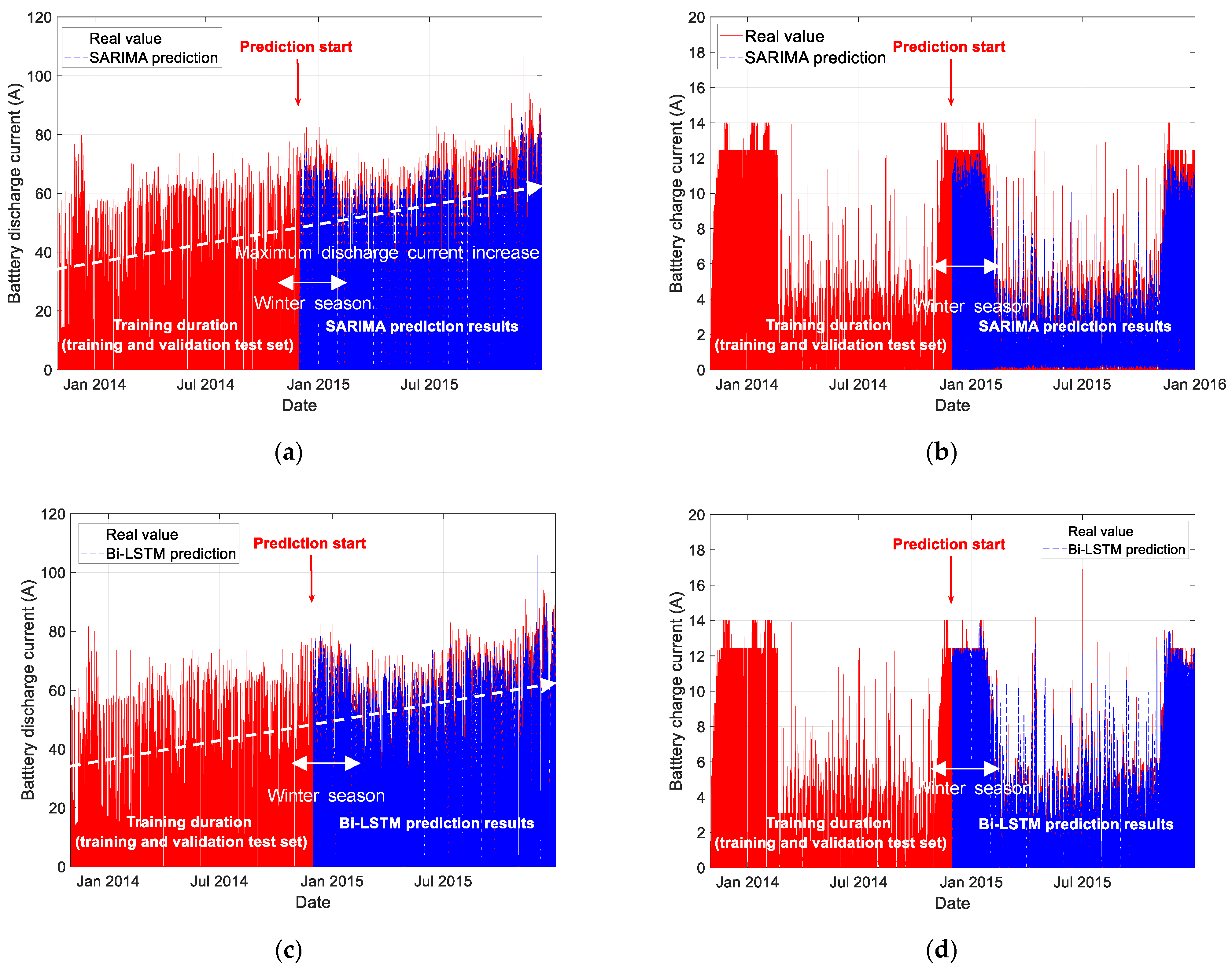
Figure 8 shows the actual battery current of the KOMPSAT-3A satellite, as well as the Bi-LSTM network and SARIMA prediction results. In the figure, the solid red line represents the actual value, and the blue dashed line shows the predicted value. Data for approximately one year after launch are used for training and validation. Then, we compare the prediction results for approximately one year. The prediction period is 12 h in consideration of the ground contact period, and this is applied equally to KOMPSAT-3A and 5. The orbit of the KOMPSAT-3A satellite has a periodic eclipse period for one year, and the maximum discharge and charge current vary depending on the change in the eclipse period, the sun irradiation, and the temperature, depending on the season.
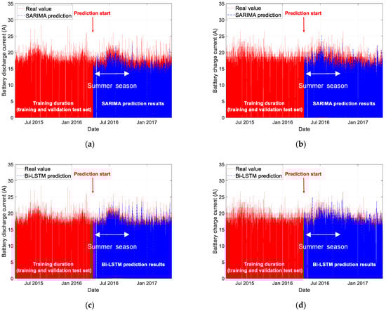
Figure 8.
KOMPSAT-3A battery charge and discharge current prediction results: (a) SARIMA results for discharge current; (b) SARIMA results for charge current; (c) Bi-LSTM results for discharge current; (d) Bi-LSTM results for charge current.
Regarding the discharge current of the KOMPSAT-3A satellite, the maximum discharge current occurs in the summer season. This is because in summer, the distance to the sun is the furthest, which reduces the power generated, which in turn increases the battery charging and discharging current. As shown in Figure 8a, SARIMA seems to estimate the seasonal change in which the maximum discharge current occurs in the summer season; however, it shows an error in the maximum discharge current value of the entire season. As shown in Figure 8c, the prediction result estimated through Bi-LSTM can estimate the trend in which the maximum discharge current occurs in summer. In addition, it can be observed that the prediction error of the maximum discharge current for one year is also relatively reduced compared to SARIMA.
The charging current is causally generated according to the discharge current, and slow charging is performed from the maximum charging current section to the tapering charging section according to the charging state. Accordingly, the amount of charging current increases in summer as does the discharge current. As shown in Figure 8b,d, the trend of the peak charging current in summer is estimated by both SARIMA and Bi-LSTM; nevertheless, the prediction error is relatively small for Bi-LSTM. In general, an increase in the maximum discharge current occurs on account of the aging of the satellite. However, in the case of the KOMPSAT-3A satellite, there is no significant change in the maximum charge and discharge current within the operating period of two years.
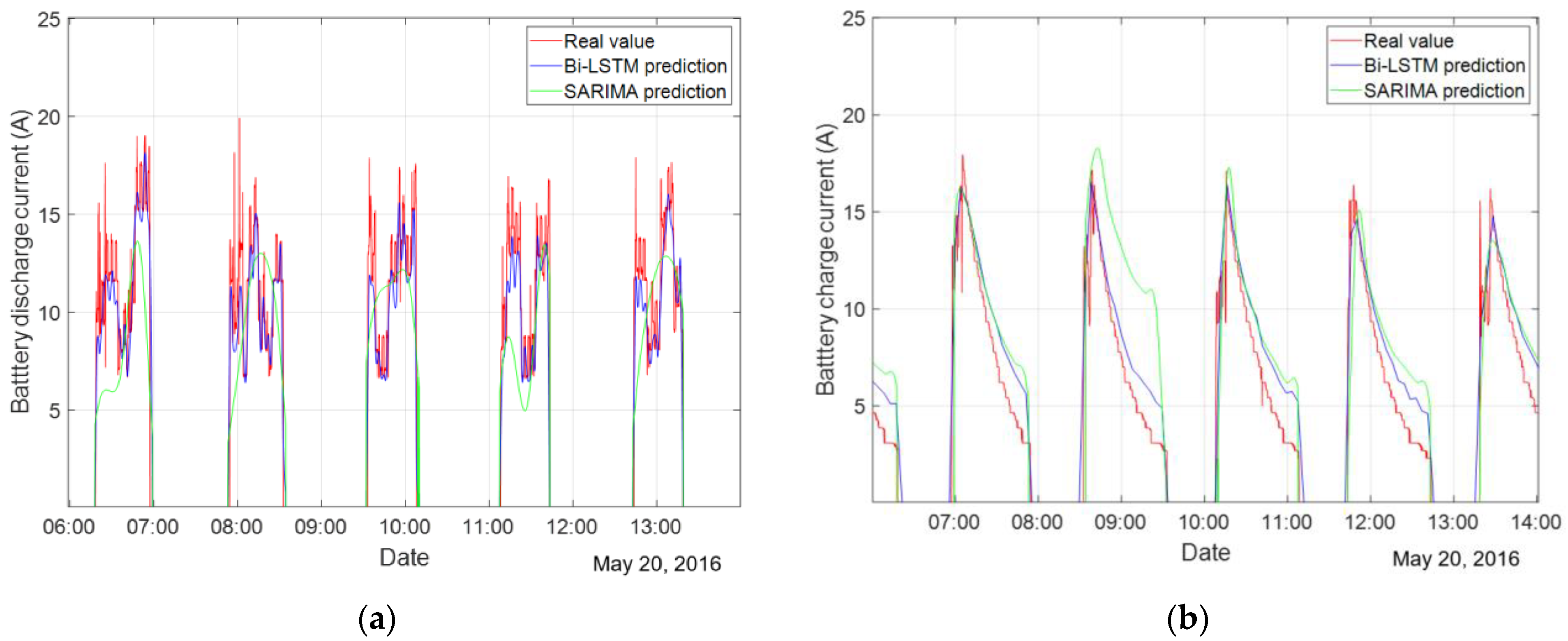
Figure 9 shows the enlarged discharge and charge current prediction results of the KOMPSAT-3A satellite, including the mission duration of 20 May 2016. Discharge occurs periodically and non-periodically by the power demand that exceeds the amount of power generated in the eclipse and mission duration. As shown in the Figure 9a, discharge usually occurs in the periodic eclipse section. It is evident that charging is performed in the sun section. In the case of Bi-LSTM, it has an error in terms of the maximum discharge current. However, it can be confirmed that it is possible to reproduce the fluctuation of the discharge current that can occur due to the attitude change and mission mode. On the other hand, in the case of the SARIMA estimation, it is not possible to reproduce the actual current fluctuation in the discharge section.
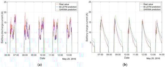
Figure 9.
KOMPSAT-3A enlarged battery current prediction results: (a) discharge current; (b) charge current.
In the case of the charging current, as shown in Figure 9b, after the eclipse period has passed, charging takes place for the duration of the sun irradiation. In the case of the KOMPSAT-3A satellite, charging is performed under the allowable charging current range of the battery, and tapering charging is performed according to the state of charge. As shown in the figure, the Bi-LSTM-based charging current is similar to the actual value compared to SARIMA. However, as shown in the estimation results from 8:30 to 9:30 in Figure 8b, a charging current prediction independent of the previous discharge amount and satellite state occurs in SARIMA, whereas in the case of Bi-LSTM, such predictions do not occur.
As observed in Figure 9, it is possible to estimate the trend in both the Bi-LSTM network and SARIMA prediction for the discharge current that occurs periodically in the eclipse section. However, the SARIMA model cannot accurately estimate the discharges that are not periodic and that cannot be specified, such as mission performance and posture changes In addition, although the charging current has a physical characteristic that varies with the discharge current, SARIMA has a prediction error with a large amount of charge current regardless of the discharge current.
Figure 10 shows the actual battery current of the KOMPSAT-5 satellite, as well as the Bi-LSTM network and SARIMA prediction results. Similar to the KOMPSAT-3A results, the red solid line represents the actual value and the blue dashed line depicts the predicted value. Similarly to the KOMPSAT-3A battery current prediction, data for one year after launch are used for learning and verification. Data from one year to two years after launch are used for prediction performance analysis, and the prediction period is selected as 12 h.

Figure 10.
KOMPSAT-5 battery charge and discharge current prediction results: (a) SARIMA results for discharge current; (b) SARIMA results for charge current; (c) Bi-LSTM results for discharge current; (d) Bi-LSTM results for charge current.
The KOMPSAT-5 satellite has an eclipse duration only in the winter season, which causes an extreme change in the charge and discharge current profile according to the season. Unlike KOMPSAT-3A, where periodic eclipses occur in all seasons, a large discharge occurs in the winter season. Furthermore, in the case of the charging current, as shown in Figure 10b,d, the winter section has a higher value than other seasons. Moreover, as shown in the figure, unlike KOMPSAT-3A, it is evident that the maximum discharge current gradually increases according to the operating period of two years.
As for Bi-LSTM estimation, the change in maximum discharge and charge current for the seasonal and operating period is similarly estimated. However, SARIMA cannot estimate the discharge current according to the mission at the correct time. Thus, an error occurs in the maximum discharge and charge current. As shown in Figure 10b,d, the charge current in the winter section is predicted to have a higher value in both SARIMA and Bi-LSTM, whereas the Bi-LSTM prediction shows a consistent and superior performance than the SARIMA.
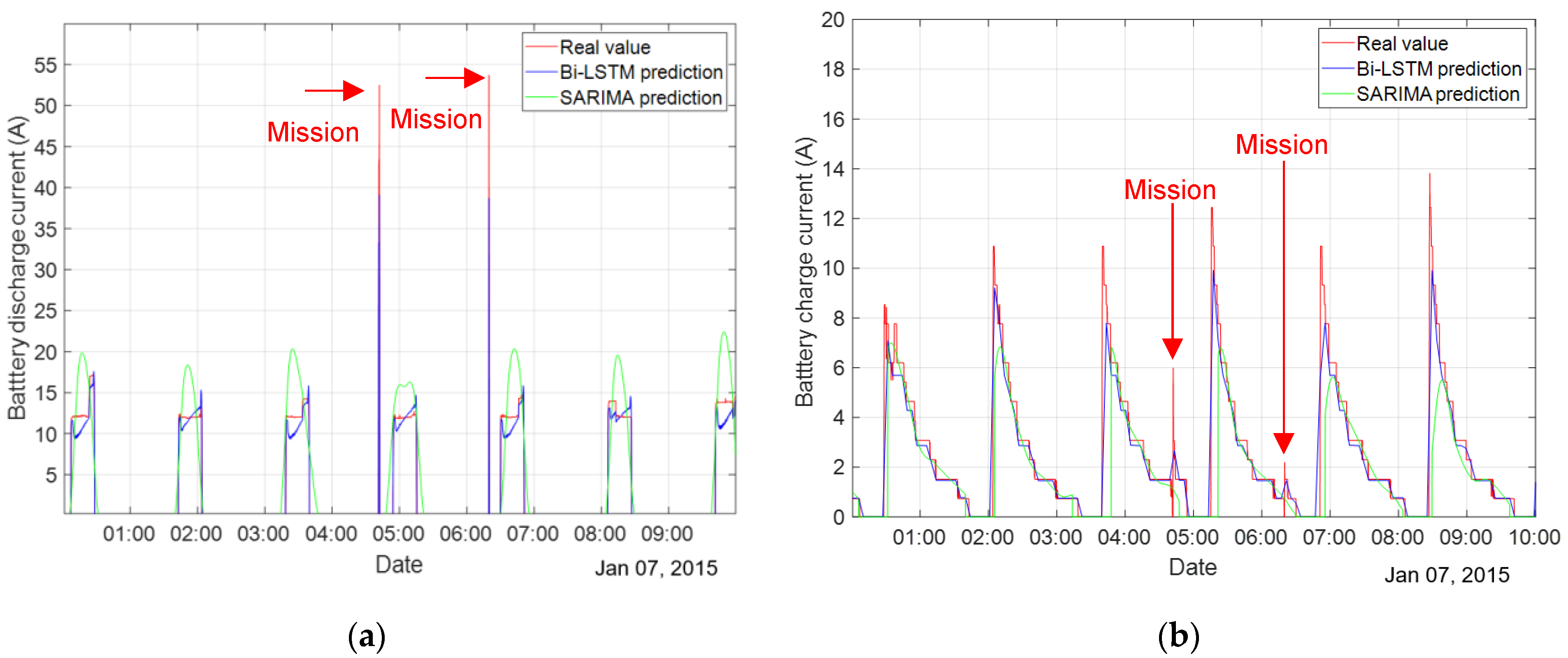
Figure 11 shows an enlarged discharge and charge current prediction results of the KOMPSAT-5 satellite, including the mission duration of 7 January 2015. In the winter section, periodic discharge occurs due to the eclipse, and the maximum discharge current appears due to the mission operation. As shown in Figure 11a, for Bi-LSTM estimation, it is possible to predict the discharge current during the non-periodic mission operation in a short time. On the other hand, with SARIMA prediction, such aperiodic discharge current prediction is not accurate, and the discharge current generated during the eclipse shows a large error compared to that of the Bi-LSTM estimation.
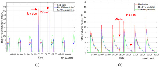
Figure 11.
KOMPSAT-3A enlarged battery current prediction results: (a) discharge current; (b) charge current.
As for charging current prediction, charging is performed in the solar section after the eclipse section has passed. Although there is a difference in accuracy, both the SARIMA model and the Bi-LSTM model predicted the shape of the waveform in which the charging current decreased according to the battery SOC. However, as found in Figure 10b, the charge current fluctuated due to the discharge current that occurred during a short period in the mission performance section, and only the Bi-LSTM model predicts this change. Thus, with Bi-LSTM model, if the maximum discharge period is estimated during the mission, the charging current is predicted utilizing the causal relationship. However, with SARIMA model, the estimation performance is poor due to the mission operation and attitude change. Therefore, through the enlarged picture, it is confirmed that the Bi-LSTM model is excellent in predicting the maximum charging and discharging current values and the predicted reproduction of the waveform.
To numerically analyze the performance of the estimation results reported in this study, we use the RMSE, MAPE, and correlation coefficient, as shown in Equations (15)–(17). The performances of the KOMPSAT-3A and KOMPSAT-5 satellite charge and discharge current simulators are examined through three indicators.
where n is the number of test data, is the actual data, is the predicted data of each model, is the mean of the , and is the mean of the
The performance is verified by classifying it into the charging and discharging duration of each satellite since the pattern repeats. Table 2 shows the seasonal performance analysis results for the battery discharge and charging current in a 12 h ahead of forecasting. As mentioned in Section 3, the prediction results for 12 h ago are analyzed considering the ground contact period of KOMPSAT-3A,5 satellites. For KOMPSAT-3A satellite, discharging and charging are performed as the eclipse duration and attitude maneuvers occur periodically. Thus, the error difference between the RMSE and MAPE of the Bi-LSTM and SARIMA is relatively small compared to that of the KOMPSAT-5 satellite. In addition, because the charge current does not change significantly with the KOMPSAT-3A satellite, there is no significant variation in the error of one year with the SARIMA model. Correlation coefficient analysis results also show that similar to RMSE and MAPE, the Bi-LSTM-based estimation results for one year are more accurate to the actual ones. For the KOMPSAT-3A satellite, the Bi-LSTM outperforms in all seasons compared with the SARIMA model, and even in the summer section where the maximum discharge current occurs.
Table 2.
The 12 h ahead prediction results.
In the prediction comparison for KOMPSAT-5 satellite, the SARIMA estimates seasonal fluctuations; however, the maximum charge and discharge current prediction error is larger than that of the Bi-LSTM model. In addition, with the SARIMA model, a more accurate estimation can be made in winter, when periodic expression intervals occur, but it is observed that larger prediction errors occur in the remaining seasons. This is because, under the assumption that the current trend would continue into the future, it does not reflect the aperiodic externalities caused by SARIMA’s limitations in predicting the future mission performance and posture change. On the contrary, with the Bi-LSTM model, it is demonstrated through the RMSE analysis result that it shows a low error than the SARIMA model in all four seasons because it could include all external variables. In addition, the similarity between the actual value and the predicted value is observed with the MAPE and correlation coefficient analysis that the Bi-LSTM prediction is superior to the SARIMA prediction.
5. Conclusions
LEO satellites have limitations in continuous status monitoring due to access restrictions in the orbit. Therefore, the development of a simulator for predicting satellite events has been undertaken. However, it is difficult to predict the state of satellites in general, because of their environmental characteristics. In particular, the power system is difficult to model mathematically because it fluctuates depending on the environment and operating conditions, such as the operating period, orbit, operating plan, and season.
In this paper, we have proposed and comparatively analyzed a technique to predict the charge and discharge current of a LEO satellite battery, which is the most important information for mission- and power-related analysis and simulator development among power systems. To confirm the validity of the proposed data-based learning technique, the on-orbit charging and discharging current prediction errors have been compared, for which training has been performed with data from one year and an evaluation has been conducted using data from the subsequent year. The performance has been demonstrated an accurate and reliable performance with real satellite data.
It is expected that data-based prediction in this study of the charging and discharging current of the satellite enables the development of a LEO satellite power simulator. Moreover, it will facilitate the development of guidelines for satellite battery management. In addition, it is anticipated that the energy balance analysis of the satellite power system can be utilized by applying the charge and discharge current predictions in this study to multiple satellites.
In the future, we plan to expand the LEO satellite battery current prediction to conduct a study on the degradation prediction of satellite power consumption and the battery SOC estimation method.
Author Contributions
All authors (S.-T.Y.; S.-H.K.) contributed equally to this work and were involved at every stage in its development. All authors have read and agreed to the published version of the manuscript.
Funding
This research received no external funding.
Conflicts of Interest
The authors declare no conflict of interest.
Abbreviations
| AR | Autoregressive |
| ARIMA | Autoregressive integrated moving average |
| BIC | Bayesian information criterion |
| Bi-LSTM | Bidirectional long short-term memory |
| BOL | Birth of life |
| IQR | Interquartile range |
| LEO | Low Earth orbit |
| LSTM | Long short-term memory |
| MA | Moving average |
| MAE | Mean absolute error |
| MAPE | Mean absolute percentage error |
| MPPT | Maximum power point tracking |
| PV | Photovoltaic |
| RMSE | Root mean square error |
| RNN | Recurrent neural network |
| SAR | Solar array regulator |
| SARIMA | Seasonal autoregressive integrated moving average |
| SEU | Single event upset |
| SOC | State of charge |
References
- Notani, S.; Bhattacharya, S. Flexible Electrical Power System Controller Design and Battery Integration for 1U to 12U CubeSats. In Proceedings of the 2011 IEEE Energy Conversion Congress and Exposition, Phoenix, AZ, USA, 17–22 September 2011; pp. 3633–3640. [Google Scholar]
- Kopacz, J.R.; Herschitz, R.; Roney, J. Small Satellites an Overview and Assessment. Acta Astronaut. 2020, 170, 93–105. [Google Scholar] [CrossRef]
- Uno, M.; Ogawa, K.; Takeda, Y.; Sone, Y.; Tanaka, K.; Mita, M.; Saito, H. Development and On-Orbit Operation of Lithium-Ion Pouch Battery for Small Scientific Satellite “REIMEI”. J. Power Sources 2011, 196, 8755–8763. [Google Scholar] [CrossRef]
- Lee, J.-W.; Anguchamy, Y.K.; Popov, B.N. Simulation of Charge-Discharge Cycling of Lithium-Ion Batteries under Low-Earth-Orbit Conditions. J. Power Sources 2006, 162, 1395–1400. [Google Scholar] [CrossRef]
- Rao, G.M.; Pandipati, R.C. Satellites: Batteries. In Encyclopedia of Electrochemical Power Sources; Elseiver: Amsterdam, The Netherlands, 2009; pp. 323–337. [Google Scholar]
- Gave, G.; Borthomieu, Y.; Lagattu, B.; Planchat, J.-P. Evaluation of a Low Temperature Li-Ion Cell for Space. Acta Astronaut. 2004, 54, 559–563. [Google Scholar] [CrossRef]
- Sinclair, D.; Dyer, J. Radiation Effects and COTS Parts in SmallSats. In Proceedings of the 27th Annual AIAA/USU Conference on Small Satellites, Logan, UT, USA, 12–15 August 2013. [Google Scholar]
- Popescu, O. Power Budgets for CubeSat Radios to Support Ground Communications and Inter-Satellite Links. IEEE Access 2017, 5, 12618–12625. [Google Scholar] [CrossRef]
- Ali, A.J.; Khalily, M.; Sattarzadeh, A.; Massoud, A.; Hasna, M.O.; Khattab, T.; Yurduseven, O.; Tafazolli, R. Power Budgeting of LEO Satellites: An Electrical Power System Design for 5G Missions. IEEE Access 2021, 9, 113258–113269. [Google Scholar] [CrossRef]
- Lee, C.-J.; Kim, B.-K.; Kwon, M.-K.; Nam, K.; Kang, S.-W. Real-Time Prediction of Capacity Fade and Remaining Useful Life of Lithium-Ion Batteries Based on Charge/Discharge Characteristics. Electronics 2021, 10, 846. [Google Scholar] [CrossRef]
- Samwel, S.W.; El-Aziz, E.A.; Garrett, H.B.; Hady, A.A.; Ibrahim, M.; Amin, M.Y. Space Radiation Impact on Smallsats during Maximum and Minimum Solar Activity. Adv. Space Res. 2019, 64, 239–251. [Google Scholar] [CrossRef]
- Ratnakumar, B.V.; Smart, M.C.; Whitcanack, L.D.; Davies, E.D.; Chin, K.B.; Deligiannis, F.; Surampudi, S. Behavior of Li-Ion Cells in High-Intensity Radiation Environments. J. Electrochem. Soc. 2004, 151, A652. [Google Scholar] [CrossRef]
- Buckle, R. Life Testing of COTS Cells for Optimum Battery Sizing. In Proceedings of the 2019 European Space Power Conference (ESPC), Juan-les-Pins, Côte d’Azur, France, 30 September–4 October 2019; pp. 1–7. [Google Scholar]
- Nguyen, H.; Hansen, C.K. Short-term electricity load forecasting with Time Series Analysis. In Proceedings of the 2017 IEEE International Conference on Prognostics and Health Management (ICPHM), Dallas, TX, USA, 19–21 June 2017; pp. 214–221. [Google Scholar] [CrossRef]
- Lee, C.M.; Ko, C.N. Short-term load forecasting using lifting scheme and ARIMA models. Expert Syst. Appl. 2011, 38, 5902–5911. [Google Scholar] [CrossRef]
- Tawfiq, A.A.E.; El-Raouf, M.O.A.; Mosaad, M.I.; Gawad, A.F.A.; Farahat, M.A.E. Optimal Reliability Study of Grid-Connected PV Systems Using Evolutionary Computing Techniques. IEEE Access 2021, 9, 42125–42139. [Google Scholar] [CrossRef]
- Ertugrul, Ö.F. Forecasting electricity load by a novel recurrent extreme learning machines approach. Int. J. Electr. Power Energy Syst. 2016, 78, 429–435. [Google Scholar] [CrossRef]
- Ding, N.; Benoit, C.; Foggia, G.; Besanger, Y.; Wurtz, F. Neural network-based model design for short-term load forecast in distribution systems. IEEE Trans. Power Syst. 2016, 31, 72–81. [Google Scholar] [CrossRef]
- Bouktif, S.; Fiaz, A.; Ouni, A.; Serhani, M. Optimal Deep Learning LSTM Model for Electric Load Forecasting using Feature Selection and Genetic Algorithm: Comparison with Machine Learning Approaches. Energies 2018, 11, 1636. [Google Scholar] [CrossRef] [Green Version]
- Xueqing, Z.; Zhansong, Z.; Chaomo, Z. Bi-LSTM Deep Neural Network Reservoir Classification Model Based on the Innovative Input of Logging Curve Response Sequences. IEEE Access 2021, 9, 19902–19915. [Google Scholar] [CrossRef]
- Li, H.; Shrestha, A.; Heidari, H.; le Kernec, J.; Fioranelli, F. Bi-LSTM Network for Multimodal Continuous Human Activity Recognition and Fall Detection. IEEE Sens. J. 2020, 20, 1191–1201. [Google Scholar] [CrossRef] [Green Version]
- Vagropoulos, S.I.; Chouliaras, G.I.; Kardakos, E.G.; Simoglou, C.K.; Bakirtzis, A.G. Comparison of SARIMAX, SARIMA, modified SARIMA and ANN-based models for short-term PV generation forecasting. In Proceedings of the 2016 IEEE International Energy Conference (ENERGYCON), Leuven, Belgium, 4–8 April 2016; pp. 1–6. [Google Scholar] [CrossRef]
- Chikkakrishna, N.K.; Hardik, C.; Deepika, K.; Sparsha, N. Short-Term Traffic Prediction Using Sarima and FbPROPHET. In Proceedings of the 2019 IEEE 16th India Council International Conference (INDICON), Rajkot, India, 13–15 December 2019; pp. 1–4. [Google Scholar] [CrossRef]
- Zheng, H.; Yuan, J.; Chen, L. Short-term load forecasting using EMD-LSTM neural networks with a Xgboost algorithm for feature importance evaluation. Energies 2017, 10, 1168. [Google Scholar] [CrossRef] [Green Version]
- Singh, P.; Dwivedi, P. Integration of new evolutionary approach with artificial neural network for solving short term load forecast problem. Appl. Energy 2018, 217, 537–549. [Google Scholar] [CrossRef]
- Chen, Y.; Luh, P.B.; Guan, C.; Zhao, Y.; Michel, L.D.; Coolbeth, M.A.; Friedland, P.B.; Rourke, S.J. Short-Term Load Forecasting: Similar Day-Based Wavelet Neural Networks. IEEE Trans. Power Syst. 2010, 25, 322–330. [Google Scholar] [CrossRef]
- Zhang, Z.; Liang, G.U.O.; Dai, Y.; Dong, X.U.; Wang, P.X. A Short-Term User Load Forecasting with Missing Data. DEStech Trans. Eng. Technol. Res. 2018. [Google Scholar] [CrossRef] [Green Version]
- Charytoniuk, W.; Chen, M.S.; Olinda, P.V. Nonparametric regression based short-term load forecasting. IEEE Trans. Power Syst. 1998, 13, 725–730. [Google Scholar] [CrossRef]
- Osborne, M. Bayesian Gaussian Processes for Sequential Prediction, Optimisation and Quadrature. Ph.D. Dissertation, Oxford University, Oxford, UK, 2010. [Google Scholar]
- Jones, D.R.; Schonlau, M.; Welch, W.J. Efficient global optimization of expensive black-box functions. J. Glob. Optim. 1998, 13, 455–492. [Google Scholar] [CrossRef]


Publisher’s Note: MDPI stays neutral with regard to jurisdictional claims in published maps and institutional affiliations. |
© 2021 by the authors. Licensee MDPI, Basel, Switzerland. This article is an open access article distributed under the terms and conditions of the Creative Commons Attribution (CC BY) license (https://creativecommons.org/licenses/by/4.0/).