Abstract
The photovoltaic (PV) system center inverter architecture comprises various conventional array topologies such as simple-series (S-S), parallel (P), series-parallel (S-P), total-cross-tied (T-C-T), bridge-linked (B-L), and honey-comb (H-C). The conventional PV array topologies under non-uniform operating conditions (NUOCs) produce a higher amount of mismatching power loss and represent multiple maximum-power-points (M-P-Ps) in the output characteristics. The performance of T-C-T topology is found superior among the conventional topologies under NUOCs. However, T-C-T topology’s main limitations are higher redundancy, more number of electrical connections, higher cabling loss, poor performance during row-wise shading patterns, and more number of switches and sensors for the re-configuration of PV modules. This paper proposes the various optimal hybrid PV array topologies to overcome the limitations of conventional T-C-T array topology. The proposed hybrid topologies are such as series-parallel-cross-tied (S-P-C-T), bridge-link-cross-tied (B-L-C-T), honey-comb-cross-tied (H-C-C-T), series-parallel-total-cross-tied (S-P-T-C-T), bridge-link-total-cross-tied (B-L-T-C-T), honey-comb-total-cross-tied (H-C-T-C-T), and bridge-link-honey-comb (B-L-H-C). The proposed hybrid topologies performance is evaluated and compared with the conventional topologies under various NUOCs. The parameters used for the comparative study are open-circuit voltage, short-circuit current, global-maximum-power-point (GMPP), local-maximum-power-point (LMPP), number of LMPPs, and fill factor (FF). Furthermore, the mismatched power loss and the conversion efficiency of conventional and hybrid array topologies are also determined. Based on the results, it is found that the hybrid array topologies maximize the power output by mitigating the effect of NUOCs and reducing the number of LMPPs.
1. Introduction
The series connection of PV cells assembles the photovoltaic (PV) module. The PV modules are connected in various possible topologies to form an array [1]. The conventional PV array topologies are simple-series (S-S), parallel (P), series-parallel (S-P), total-cross-tied (T-C-T), bridge-linked (B-L), and honey-comb (H-C) [2,3,4,5]. The power output from conventional PV array topologies is significantly reduced and produces mismatched power loss under partial shading conditions. Generally, Partial shades are caused by the moving clouds, shadows of buildings, bird droppings, trees, poles, chimneys, power lines, and so on [6]. The mismatching power loss is due to non-uniform operating conditions (NUOCs) of PV modules within the array, aging phenomena, potential induced degradation (PID) effect, thermal defects, and so on [7]. The mismatched power loss can be partially mitigated by connecting an anti-parallel bypass diode to each PV module in an array [8]. However, the presence of bypass diode connection results in more numbers of maximum-power-points in the I-V and P-V characteristics of array topologies [9]. The various other approaches to mitigate the effect of NUOCs are PV array topologies [10,11,12,13], modified maximum-power-point-tracking (M-P-P-T) techniques [14,15,16,17], PV system architectures [18,19,20,21] and the use of multi-level power electronic converters [22,23,24,25,26,27,28,29,30,31,32,33].
The primary and more straightforward solution to mitigate the effect of NUOCs is the selection of appropriate PV array topology. S.R. Pendem et al., evaluated the performance of symmetrical S-S, P, S-P, T-C-T, B-L, and H-C topologies, and the authors determined that T-C-T topology under NUOCs reducing the mismatching power loss as compared to the other topologies [34]. N. K. Gautam et al., assessed the reliability and the operational lifetime of bigger size asymmetrical S-P, T-C-T, and B-L topologies by concerning the manufacturing tolerances. The authors found that T-C-T topology’s reliability and lifetime are superior over S-P and B-L [35]. M. John Bosco et al., and P.K. bonthagorla et al., proposed an optimal cross-diagonal-view (C-D-V) and triple-tied (T-T) topologies with a reduced number of cross-ties to mitigate the effect of NUOCs [36,37]. K. Lappalainen et al., assessed the performance of various asymmetrical size (, , and ) S-P and T-C-T topologies. The parameters considered to determine the performance of PV array topologies are the variations in the insolation transition characteristics such as shade strength, duration of shade, the apparent speed of shade, and the direction of movement of shadow. The results show that mismatching power loss during insolation transitions is practically the same [38]. P. S. Rao et al., proposed a novel static reconfiguration technique to T-C-T topology for distributing the effect of NUOCs over the entire array without change of physical location of the modules. The results show that the proposed technique exhibits exceptional performance over S-P, T-C-T, and B-L topologies [39]. M. Horoufiany et al., proposed an optimal static reconfiguration technique to T-C-T topology under mutual shading conditions. The functioning of the proposed approach is remarkable than the T-C-T and Sudoku arrangements. This technique needs dispersion of more number of modules in an array. Thus, the length of the cabling is more than the T-C-T and Sudoku arrangements [40]. Futoshiki Sudoku, optimal Sudoku, unsymmetrical puzzle, zig-zag, dominant square logic, and improved magic square techniques have been proposed to improve the performance of T-C-T topology [41,42,43,44,45,46,47]. The shade dispersion static reconfigured techniques do not require any sensors, reconfiguration algorithm, and switching matrix. However, this technique needs laborious work, excessive interconnecting ties, and an adequate reconfigurable pattern to distribute the shading effect.
Nguyen et al., proposed an adaptive reconfiguration technique to T-C-T topology by employing a model-based sorting algorithm. It consists of a fixed and adaptive PV array, a few voltage and current sensors, electro-mechanical switches, switching matrix, and an intelligent controller [48]. Quesada et al., implemented an electrical array reconfiguration (EAR) method in which the connections of PV modules dynamically changed as stated by a controllable switching matrix. Though the power loss decreased under NUOCs, this method is relevant to only small-scale installations. Furthermore, it associates with higher cost and greater complexity [49]. S. N. Deshkar et al., recommended genetic algorithm (GA) based EAR arrangement to T-C-T topology. The GA-based EAR technique results show superior performance over the sudoku pattern technique. However, this arrangement’s inherent drawbacks are poor convergence, large computational steps, extensive search, and requires an active switching matrix [50]. T. S. Babu et al., proposed particle swarm optimization (PSO) based EAR strategy to T-C-T topology. The performance of this technique was tested based on parameter tuning, payback period, algorithm complexity, switching arrangement, sensor requirement, and wiring complexity [51]. Subsequently, the authors in [52,53,54,55] handled the EAR technique to T-C-T topology for improved power generation. Even though an EAR’s functioning is significant over static reconfiguration, the limitations of the EAR technique are greater complexity and cost since it requires a large number of switches and sensors, a controllable switching matrix, and an intelligent micro-controller.
Al-Motasem I. Aldaoudeyeh et al., proposed a shading compensation technique to T-C-T topology to alter the P–V characteristics of shaded arrays to become closer to the non-shaded ones, and the results show that the compensation technique enhances the maximum power of shaded arrays by 5% to 58%. Each row of the PV modules in a T-C-T topology requires a battery, charge controller, three switches, and two diodes [56]. P. Sharma et al., proposed a shunt-series compensation method to array topologies. This method is intended to operate the shaded PV modules at their actual maximum-power-point (M-P-P) despite NUOCs. A fly-back converter is connected in shunt with each of the PV modules for compensating the row currents. Another fly-back converter is connected in series with each of the strings for compensating voltage differences. This method requires more electro-mechanical relays, power electronic converters, intelligent string controller (ISC), and intelligent array controller (IAC). It is found that the proposed method is not efficient for the full-power processing architectures [57]. Therefore, as per the literature, T-C-T topology exhibits less sensitivity to NUOCs and generates the highest maximum power compared to the other conventional topologies. Even though the reliability of the T-C-T topology is more, it requires more electrical connections between the PV modules. Hence, the cabling cost and also the wiring loss of the T-C-T topology are higher. If any of the electrical connections between the two modules in a row is open-circuited/failed, then the performance of the T-C-T topology reduces. The significant issues with the T-C-T topology are poor performance during row-wise shading patterns, more interconnections that increase the power loss, mismatched power loss, higher redundancy, and need more switches and sensors to re-configuration of PV modules.
This research paper proposes various optimal hybrid PV array topologies to overcome T-C-T topology limitations. The proposed hybrid topologies are series-parallel-cross-tied (S-P-C-T), bridge-link-cross-tied (B-L-C-T), honey-comb-cross-tied (H-C-C-T), series-parallel-total-cross-tied (S-P-T-C-T), bridge-link-total-cross-tied (B-L-T-C-T), honey-comb-total-cross-tied (H-C-T-C-T), and bridge-link-honey-comb (B-L-H-C). The mathematical formulations to the proposed hybrid topologies for calculating the output voltage, current, and power are also designated. Further, the performance of the proposed hybrid topologies is investigated and also compared with the conventional S-P, B-L, and H-C array topologies under uneven-row, uneven-column, diagonal, short and narrow (SAN), short and wide (SAW), long and narrow (LAN), long and wide (LAW), center, and random NUOCs. The various parameters used for the comparative study are open-circuit voltage, short-circuit current, GMPP parameters, LMPP parameters, no. of peaks, fill factor (FF), mismatching power loss, and the conversion efficiency.
The rest of this research paper’s sections are organized as follows: Section 2 describes the mathematical modeling of the PV module two-diode model. The modeling and mathematical formulations of the conventional & proposed hybrid array topologies are presented in Section 3. The explanation about the different types of considered NUOCs is presented in Section 4. The results and discussion about the performance analysis of conventional & proposed hybrid array topologies are given in Section 5. Finally, a brief conclusion about the proposed hybrid array topology’s performance is given in Section 6.
2. PV Module Two-Diode Model
The PV cell is the primary device for the generation of electricity from PV systems. Figure 1 demonstrate the different types of electrical equivalent circuits of PV module [58]. Figure 1a shows the ideal equivalent circuit of PV module comprises a controlled current source parallel to a diode. The ideal model improved with the addition of series resistance () as shown in Figure 1b and is considered as a simplified model. The simplified model shows significant flaws if the temperature variations are observed. Hence, the simplified model also improved with the inclusion of shunt resistance () [59]. The accuracy of the improved single-diode model deteriorates at low insolation. Furthermore, the equivalent circuit of a single-diode model assumes that the recombination loss of charge carriers is absent in the depletion region. However, in practical cases, at low voltages, the recombination of charge carriers represents a significant loss. Hence, the PV module two-diode model shown in Figure 1c is introduced, which includes the recombination loss [60,61]. The mathematical modeling of the PV module two-diode model is described with Equations (1)–(3).
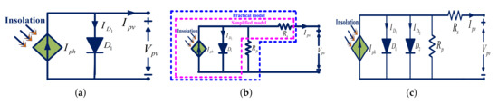
Figure 1.
PV module equivalent circuits. (a) Ideal model, (b) simplified and practical model, and (c) two-diode model.
- Equation (1) demonstrates the relation between output current and output voltage of a PV module:
In Equation (2), is the photo-generated current at standard test condition (STC) of 1000 W/m and 25 C; and G are the solar insolation at STC and at any considered insolation; is the temprature coefficient of short-circuit current; = is the change in temperature; T and are the ambient temperature and temperature at STC.
- The diode reverse saturation currents, and are expressed by the Equation (3).
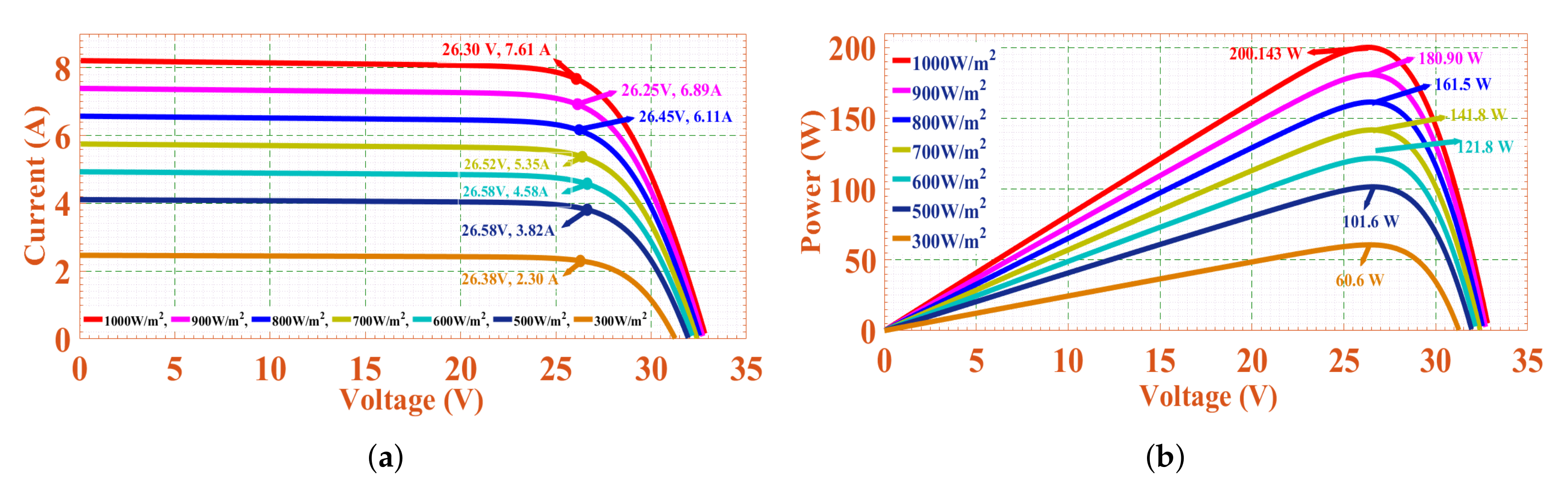
In Equation (3), & are the open-circuit voltage and short-circuit current at STC; and is the temperature coefficient of open-circuit voltage. The value of must be unity, ⩾ 1.2, and p⩾ 2.2. This paper considers the KC200GT poly-crystalline module parameters for modeling the PV module in MATLAB/Simulink [62]. The output characteristics of the KC200GT PV module at various insolation levels are represented in Figure 2.
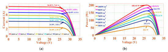
Figure 2.
KC200GT PV module output characteristics. (a) I–V, and (b) P–V characteristics.
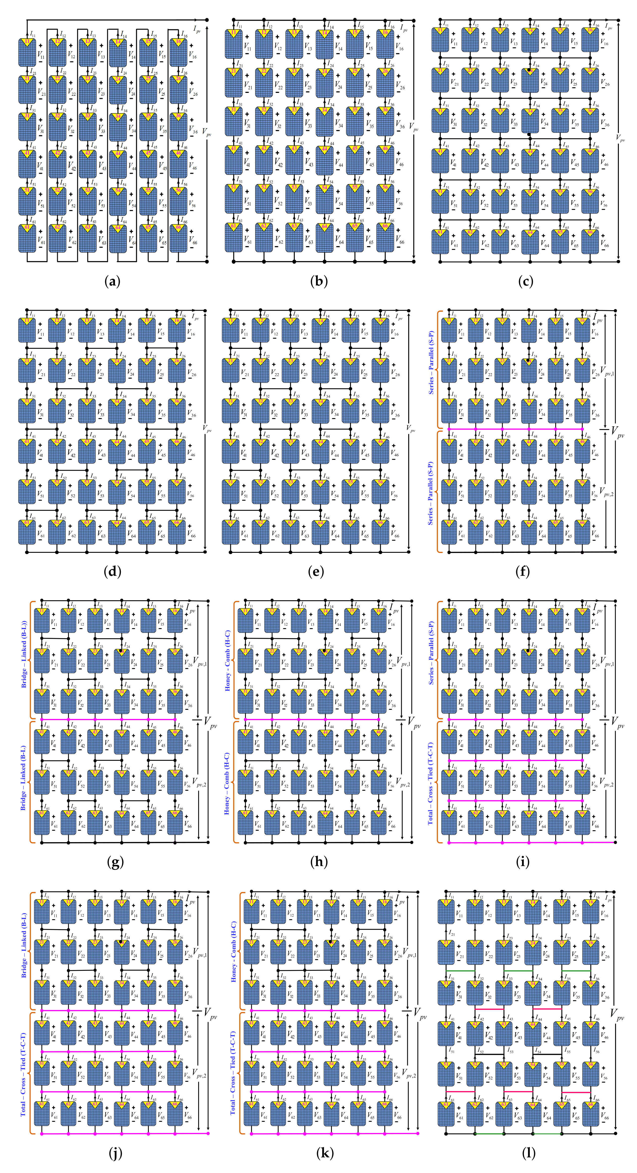
3. Conventional and Proposed Optimal Hybrid PV Array Topologies
This section describes the modeling and mathematical analysis of conventional and proposed optimal hybrid PV array topologies. The conventional topologies S-S, S-P, T-C-T, B-L, and H-C, are shown in Figure 3a–e. The proposed hybrid topologies S-P-C-T, B-L-C-T, H-C-C-T, S-P-T-C-T, B-L-T-C-T, H-C-T-C-T, and B-L-H-C, are shown in Figure 3f–l. The hybrid topologies are modeled by connecting any two of the conventional topologies with a cross-tied connection. The conventional and hybrid topologies comprise six rows and six columns of PV modules. An anti-parallel bypass diode connected to each PV module in both the conventional and hybrid array topologies. The positions of PV modules in each row and column of all the topologies are numbered as (11, 12, …, 16), (21, 22, …, 26), (31, 32, …, 36), (41, 42, …, 46), (51, 52, …, 56) and (61, 62, …, 66), respectively, [2,3,4,5]. The output voltage of all PV modules numbered from 11, 12, 13, …, 65 to 66 is represented by and ; whereas the currents are represented by and , respectively. For example, the position of the module in the 4th row and 6th column of a topology represented with a number ’46’, and its output voltage and current are represented by and , respectively. The array output voltage and current represented by and , respectively. The description of both the conventional and hybrid topologies is as follows:
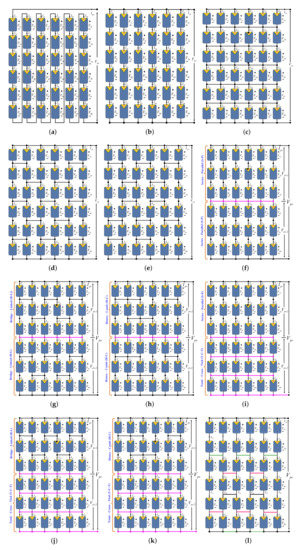
Figure 3.
Conventional and proposed hybrid PV array topologies: (a) simple-series (S-S), (b) series-parallel (S-P), (c) total-cross-tied (T-C-T), (d) bridge-linked (B-L), (e) honey-comb (H-C), (f) series-parallel-cross-tied (S-P-C-T), (g) bridge-linked-cross-tied (B-L-C-T), (h) honey-comb-cross-tied (H-C-C-T), (i) series-parallel-total-cross-tied (S-P-T-C-T), (j) bridge-linked-total-cross-tied (B-L-T-C-T), (k) honey-comb-total-cross-tied (H-C-T-C-T), and (l) bridge-linked-honey-comb (B-L-H-C).
3.1. Conventional PV Array Topologies
3.1.1. Series-Parallel (S-P)
The S-P topology shown in Figure 3b is the most commonly used for stand-alone and grid-connected PV system applications. The PV modules are connected like a string to attain the required output voltage, and the strings are connected in parallel to achieve the necessary output current. The S-P topology output current equals the sum of strings current, and the output voltage is equal to the voltage across the strings. The performance of the S-P topology is superior over T-C-T under row-wise NUOCs. This topology’s limitations are more peaks and lower maximum power generation capability than cross-tied connections under most of the NUOCs.
3.1.2. Total-Cross-Tied (T-C-T)
As shown in Figure 3c, the T-C-T topology is assembled by connecting all the rows with a cross-tied connection. The modules in a row are parallel-connected because of the cross-tied connection, and the rows series-connected. The T-C-T topology output current is equal to the sum of module currents in any row, and the output voltage is equal to the sum of voltages across all the rows. The advantages of T-C-T topology are longer operational lifetime, lesser multi-peak effect, good fault-tolerant, and higher power generation capability under most of the NUOCs.
3.1.3. Bridge-Link (B-L)
The B-L topology is shown in Figure 3d. Every four PV module in this topology is connected similarly to the bridge-rectifier fashion. For example, the PV modules numbered ’21’ and ’31’ are series-connected and joined parallel to the series connection of ’22’ and ’32’. In Figure 3d, a total of eleven B-L’s are present. B-L topology’s advantages are slightly longer operational lifetime and higher power generation capability than the S-P and T-C-T under a ladder and column-wise NUOCs.
3.1.4. Honey-Comb (H-C)
The modified version of the B-L topology is shown in Figure 3e and is referred to as H-C. Each H-C structure comprises six PV modules, where the first three modules are series-connected and then connected in parallel to another three series-connected modules (S-P combination). This S-P topology’s top and bottom nodes are connected to another S-P topology comprising two PV modules. For example, in Figure 3e, the S-P topology of modules numbered (23, 33, 43, 24, 34, 44) are connected at the top of bottom nodes of other S-P combinations of modules numbered (13, 14) and (53, 54). The performance of the H-C topology is superior to T-C-T for asymmetrical array sizes. Its performance is also outstanding over T-C-T under row-wise NUOCs.
3.2. Hybrid PV Array Topologies
3.2.1. Series-Parallel-Cross-Tied (S-P-C-T)
The S-P-C-T topology shown in Figure 3f is modeled by combining two symmetrical sections of S-P topologies. The symmetrical sections of S-P topologies are cross-tied (pink colored line). In Figure 3f, the PV modules (31, 32, 33, 34, 35, 36) and (41, 42, 43, 44, 45, 46) are connected at the same node. Hence, both the symmetrical sections of S-P topologies are in series connection. Thus, the same current flows through both the symmetrical S-P topologies. The S-P-C-T topology output voltage is equal to the sum of voltages across both the S-P topologies. The performance of the S-P-C-T topology is superior to the S-P topology. S-P-C-T topology’s advantages are lesser redundancy, a lesser number of connections, and lower cabling loss.
3.2.2. Bridge-Link-Cross-Tied (B-L-C-T)
It is modeled by combining two of the symmetrical sections of B-L topologies, and both the symmetrical sections are series-connected, as shown in Figure 3g. Thus, the same current will flow through the B-L topologies sections. Each of the B-L topologies comprises five B-L structures. The performance of the B-L-C-T topology is superior over S-P and B-L topologies.
3.2.3. Honey-Comb-Cross-Tied (H-C-C-T)
The H-C-C-T topology shown in Figure 3h is modeled by combining two symmetrical sections of the H-C topologies in a series connection. Thus, the same current flows through both the H-C topologies. Each of the H-C topology comprises three H-C structures. H-C-C-T topology advantages are superior performance over S-P, B-L, and H-C topologies.
3.2.4. Series-Parallel-Total-Cross-Tied (S-P-T-C-T)
As shown in Figure 3i, the S-P-T-C-T topology is modeled by the series connection of S-P and T-C-T topologies. Thus, the same current flows through the S-P and T-C-T topologies. The S-P topology is modeled with the modules (11, 21, 31), (12, 22, 32), (13, 23, 33), (14, 24, 34), (15, 25, 35), and (16, 26, 36), and the T-C-T topology is modeled with the modules (41, 42, 43, 44, 45, 46), (51, 52, 53, 54, 55, 56), and (61, 62, 63, 64, 65, 66). S-P-T-C-T topology performance is superior over S-P, B-L, H-C, and S-P-C-T topologies under most NUOCs.
3.2.5. Bridge-Link-Total-Cross-Tied (B-L-T-C-T)
It is modeled by the series connection of B-L and T-C-T topologies, as shown in Figure 3j. Thus, the same current flows through the B-L and T-C-T topologies. The B-L topology modeled with the modules numbered (21, 22, 31, 32), (12, 13, 22, 23), (23, 24, 33, 34), (14, 15, 24, 25), and (25, 26, 35, 36). The T-C-T topology is modeled with the modules same as in the S-P-T-C-T topology. The B-L-T-C-T topology performance is superior over S-P, B-L, H-C, S-P-C-T, and B-L-C-T topologies.
3.2.6. Honey-Comb-Total-Cross-Tied (H-C-T-C-T)
The H-C-T-C-T topology shown in Figure 3k is modeled by the series connection of H-C and T-C-T topologies. Thus, the same current will flow through the H-C and T-C-T topologies. The H-C topology modeled with the modules (21, 22, 31, 32, 12, 13), (32, 33, 13, 14, 23, 24), and (14, 15, 24, 25, 34, 35). The T-C-T topology modeled with the modules same as in the S-P-T-C-T and B-L-T-C-T topology. H-C-T-C-T topology performance is superior over S-P, B-L, H-C, S-P-C-T, and B-L-C-T topologies.
3.2.7. Bridge-Link-Honey-Comb (B-L-H-C)
As shown in Figure 3l, it is seen that B-L-H-C topology is a series combination of both the B-L and H-C structures. The modules (11, 12, 21, 22), (52, 53, 62, 63), (13, 14, 23, 24), (54, 55, 64, 65) and (15, 16, 25, 26) assembles the B-L structures, whereas the modules (31, 32, 41, 42, 51, 52), (12, 13, 22, 23, 32, 33), (33, 34, 43, 44, 53, 54), (14, 15, 24, 25, 34, 35) and (35, 36, 45, 46, 55, 56) assembles the H-C structures [63,64]. The B-L-H-C topology shown in Figure 3l comprises five number of B-L and H-C structures.
The PV array topologies output voltage and current in terms of module output voltages and currents are expressed in Table 1.

Table 1.
Conventional and proposed hybrid PV array topologies output voltage and output current formulations.
4. Modeling of Non-Uniform Operating Conditions
The main objective of this paper is to analyze the performance of both the conventional and hybrid topologies under various NUOCs such as uneven-row, uneven-column, diagonal, short-and-narrow (SAN), short-and-wide (SAW), long-and-narrow (LAN), long-and-wide (LAW), center, and random. The NUOCs comprises various insolation levels such as 300 W/m, 400 W/m, 500 W/m, 700 W/m, 800 W/m, 900 W/m and 1000 W/m. Figure 4 shows the type of NUOC and represents the corresponding insolation level in each NUOC. The description of each of the considered NUOCs is given as follows:
- Uneven-row: As shown in Figure 4a, the first row of array PV topologies is unevenly shaded with different insolation levels. The PV modules (11, 12), (13, 14) and (15, 16) receives an insolation of 300 W/m, 500 W/m and 700 W/m, respectively. The rest of all PV modules receives insolation of 1000 W/m.
- Uneven-column: The first column of PV array topologies is unevenly shaded with different insolation levels, as shown in Figure 4b. The PV modules (11, 21), (31, 41), and (51, 61)receives an insolation of 300 W/m, 500 W/m and 700 W/m, respectively. The rest of all the PV modules receives insolation of 1000 W/m.
- Diagonal: The diagonally placed PV modules are shaded with different insolation levels, as shown in Figure 4c. The PV modules 11, 22, 33, 44, 55, and 66 receives an insolation of 300 W/m, 400 W/m, 500 W/m, 700 W/m, 800 W/m and 900 W/m, respectively. The rest of all the PV modules receives insolation of 1000 W/m.
- Short and Narrow (SAN): As shown in Figure 4d, a fewer number of PV modules in the first three rows of array topologies are shaded with different insolation levels. The PV modules (11, 12, 13), (21,22, 23) and (31, 32, 33) receives an insolation of 300 W/m, 500 W/m and 700 W/m, respectively. The rest of all the PV modules receives insolation of 1000 W/m.
- Short and Wide (SAW): All the PV modules in the first three rows of array topologies are shaded with different insolation levels as shown in Figure 4e. The PV modules (11, 12, 21, 22), (13, 14, 23, 24), (15, 16, 25, 26) and (31, 32, 33, 34, 35, 36) receives an insolation of 300 W/m, 500 W/m, 700 W/m and 900 W/m, respectively. The rest of all the PV modules receives an insolation of 1000 W/m.
- Long and Narrow (LAN): The PV modules in the first two columns of array topologies are shaded with different insolation levels, as shown in Figure 4f. The PV modules (11, 12, 21), (22, 31, 32), (41, 42, 51) and (52, 61, 62) receives an insolation of 300 W/m, 500 W/m, 700 W/m and 900 W/m, respectively. The rest of all the PV modules receives insolation of 1000 W/m.
- Long and Wide (LAW): The PV modules in the first five columns of array topologies are shaded with different insolation levels as shown in Figure 4g. The PV modules (11, 12, 21, 22, 31, 32), (13, 14, 23, 24, 33, 34), (15, 25, 35), (41, 42, 51, 52, 61, 62), (43, 44, 54, 55, 64, 65) and (45, 55, 65) receives an insolation of 300 W/m, 500 W/m, 600 W/m, 700 W/m, 800 W/m and 900 W/m, respectively. The rest of all the PV modules receives an insolation of 1000 W/m.
- Random: As shown in Figure 4h, a fewer number of PV modules in all the six rows of array topologies are shaded with different insolation levels. The PV modules (26, 31, 44, 52, 65), (15, 21, 36, 53, 64), (14, 23, 35, 41, 63) and (12, 33, 45, 54, 56) receives an insolation level of 300 W/m, 500 W/m, 700 W/m and 900 W/m, respectively. The rest of all the PV modules receives an insolation of 1000 W/m.
- Center: As shown in Figure 4i, the PV modules in array topologies placed at the center of fewer rows are shaded with different insolation levels. The PV modules numbered (23, 24), (33, 34), (43, 44) and (53, 54) receives an insolation of 300 W/m, 500 W/m, 700 W/m and 900 W/m, respectively. The rest of all the PV modules receives insolation of 1000 W/m.
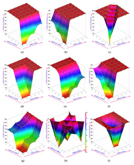
Figure 4.
Representation of various shading patterns and corresponding insolation levels on PV array topologies: (a) uneven-row, (b) uneven-column, (c) diagonal, (d) SAN, (e) SAW, (f) LAN, (g) LAW, (h) random, and (i) center.
Figure 4.
Representation of various shading patterns and corresponding insolation levels on PV array topologies: (a) uneven-row, (b) uneven-column, (c) diagonal, (d) SAN, (e) SAW, (f) LAN, (g) LAW, (h) random, and (i) center.

5. Results and Disucussion
This section describes the results of both the conventional and proposed optimal hybrid PV array topologies under various shading patterns discussed in Section 4. Figure 5, Figure 6, Figure 7, Figure 8, Figure 9, Figure 10, Figure 11, Figure 12, Figure 13 and Figure 14 shows the results of S-P, B-L, H-C, S-P-C-T, B-L-C-T, H-C-C-T, S-P-T-C-T, B-L-T-C-T, H-C-T-C-T, and B-L-H-C topologies. The performance of proposed hybrid topologies compared with the conventional array topologies. The comparative analysis is based on the parameter variations of open-circuit voltage (), short-circuit current (), GMPP parameters (, , and ), LMPP parameters, no. of peaks, fill factor (FF), mismatching power loss () and conversion efficiency () of topologies. The main parameters to assess the performance of any array topology is the and . The Equations (4) and (5) give the expressions to determine the and , respectively. The amount of GMPP generated under every shading pattern is related to the product of and of a PV array topology, and it is referred to as the fill factor (FF). Equation (6) gives the expression to determine the FF.
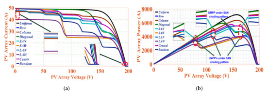
Figure 5.
Results of S-P topology under various PSCs. (a) I-V characteristics, and (b) P-V characteristics.

Figure 6.
Results of B-L topology under various PSCs. (a) I-V characteristics, and (b) P-V characteristics.
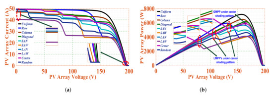
Figure 7.
Results of H-C topology under various PSCs. (a) I-V characteristics, and (b) P-V characteristics.

Figure 8.
Results of S-P-C-T topology under various PSCs. (a) I-V characteristics, and (b) P-V characteristics.
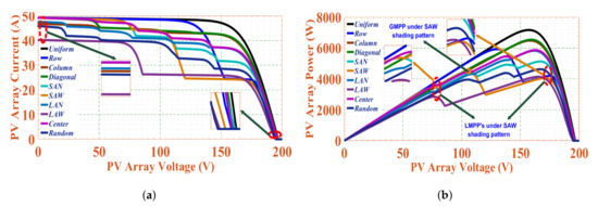
Figure 9.
B-L-C-T topology results under various PSCs. (a) I-V characteristics, and (b) P-V characteristics.
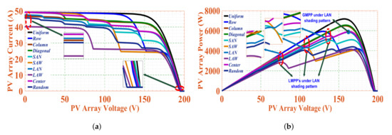
Figure 10.
H-C-C-T topology results under various PSCs. (a) I-V characteristics, (b) P-V characteristics.

Figure 11.
S-P-T-C-T topology results under various PSCs. (a) I-V characteristics, (b) P-V characteristics.
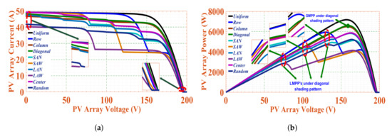
Figure 12.
B-L-T-C-T topology results under various PSCs. (a) I-V characteristics, (b) P-V characteristics.
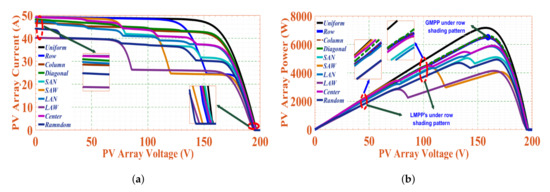
Figure 13.
H-C-T-C-T topology results under various PSCs. (a) I-V characteristics, (b) P-V characteristics.
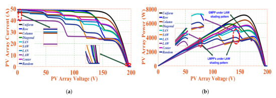
Figure 14.
B-L-H-C topology results under various PSCs. (a) I-V characteristics, (b) P-V characteristics.
The parameters in the Equations (4)–(6) are defined as follows: , , , and are the power generated at STC, GMPP under partial shading condition, no. of PV modules, and insolation level on an array topologies at STC. ’A’ is the area of a PV module.
5.1. Under Uniform Shading Pattern
Every PV module in all the array topologies receives insolation of 1000 W/m under a uniform shading pattern. Both the conventional and proposed hybrid topologies under this shading pattern operate at and of 196.60 V and 49.26 A, respectively. All PV array topologies under this shading pattern generate only one peak in the characteristics at 7205.15 W (GMPP). The corresponding and of all the PV array topologies at GMPP are 157.04 V and 45.88 A, respectively. The FF and of all array topologies under this shading pattern is at 0.742% and 14.15%, respectively.
5.2. Under Uneven-Row Shading Pattern
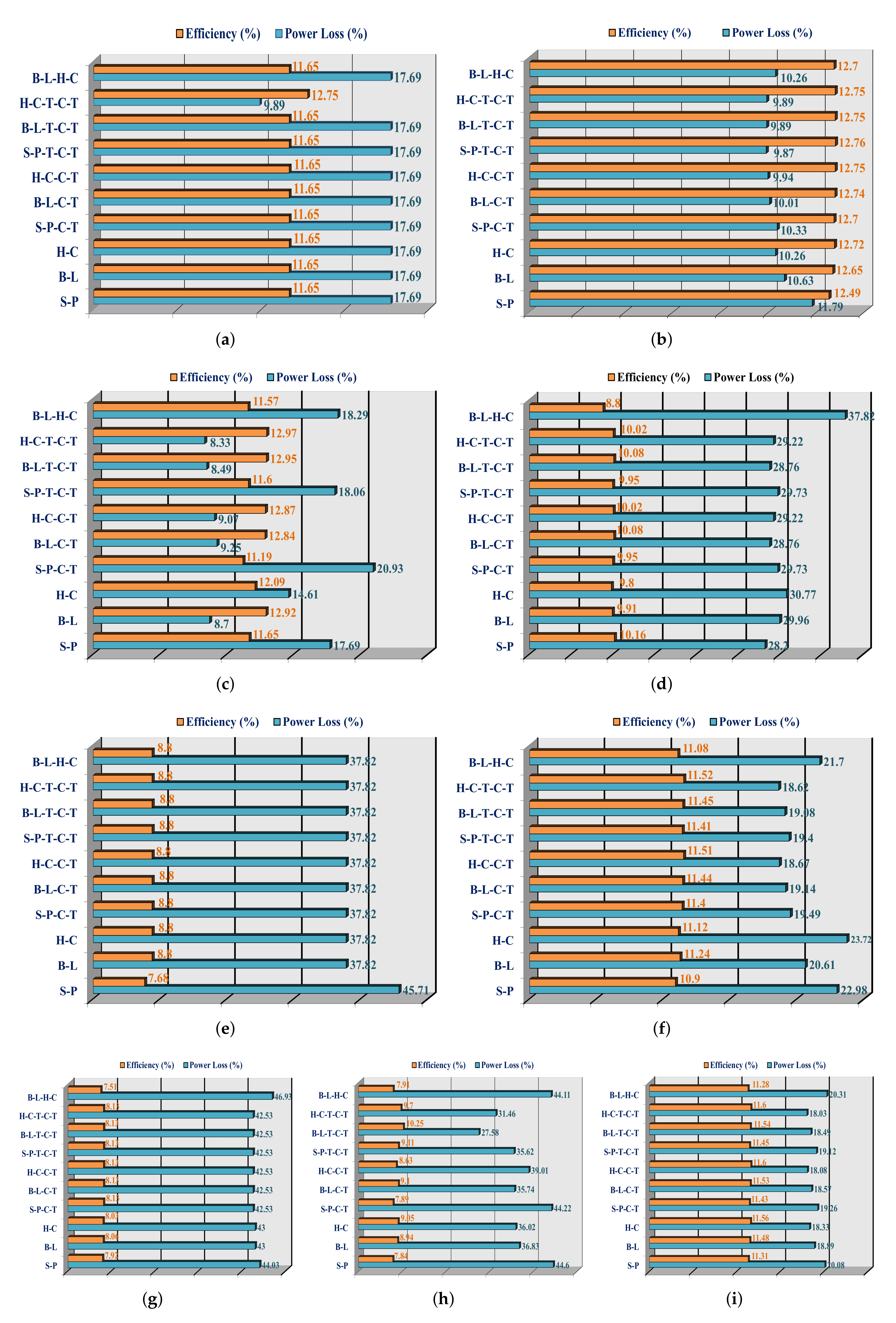
Both the conventional and hybrid array topologies under uneven-column shading patterns operate at a of 49.26 A. The H-C-T-C-T topology generates the highest GMPP at 6492.75 W. The corresponding and of H-C-T-C-T topology at GMPP are 157.04 V and 41.01 A, respectively. The H-C-T-C-T topology represents two LMPPs in the output characteristics. The operating power, voltage, and current at the LMPP’s of H-C-T-C-T topology are at (1971.88 W, 43.30 V, 45.54 A) and (4438.85 W, 100.70 V, 44.08 A), respectively. The rest of the topologies generate a GMPP of 5930.80 W and represent only one number of LMPP. The , and of H-C-T-C-T topology under uneven-column shading pattern are 9.42%, 12.75% and 0.67, respectively. The parameter variations of both the conventional and hybrid topologies under this shading pattern are represented in Table 2. The calculated values of and of both the conventional and proposed hybrid topologies are represented in Figure 15a.
Table 2.
Parameter variations of conventional and hybrid configurations under uneven-row pattern.

Figure 15.
Efficiency and mismatching power losses of conventional and proposed hybrid topologies under various shading patterns: (a) uneven-row, (b) uneven-column, (c) diagonal, (d) SAN, (e) SAW, (f) LAN, (g) LAW, (h) random, and (i) center.
5.3. Under Uneven-Column Shading Pattern
The H-C-T-C-T topology under uneven-column shading pattern generates the highest GMPP at 6498.15 W. The corresponding and of H-C-T-C-T topology at GMPP are 158.32 V and 41.01 A, respectively. The H-C-T-C-T topology represents two LMPP’s at an operating power, voltage, and current same as the under uneven-row shading pattern. The calculated values of and of both the conventional and proposed hybrid topologies are represented in Figure 15b. The S-P, B-L, H-C, S-P-C-T, B-L-C-T, B-L-T-C-T, and B-L-H-C topologies also represented two LMPP’s, whereas the H-C-C-T and S-P-T-C-T represent only one LMPP. The S-P topology performance is lower than the rest of the topologies, and its operating points at GMPP are (6355.80 W, 157.56 V, 40.34 A). The , and of H-C-T-C-T topology under uneven-column shading pattern are 9.42%, 12.75% and 0.67, respectively. The parameter variations of both the conventional and hybrid topologies under uneven-column shading patterns are represented in Table 3.
Table 3.
Parameter variations of conventional and hybrid configurations under uneven-column pattern.
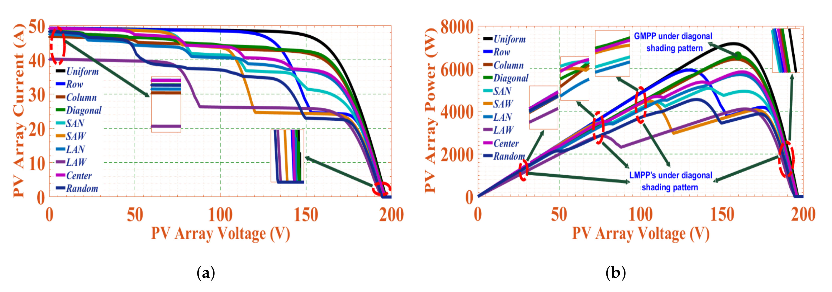
5.4. Under Diagonal Shading Pattern
The parameter variations of both the conventional and hybrid PV array topologies under diagonal shading patterns are represented in Table 4. The calculated values of and of both the conventional and hybrid topologies are represented in Figure 15c. The H-C-T-C-T topology generates the highest GMPP at 6605.05 W. The corresponding and of an H-C-T-C-T topology at GMPP are 159.19 V and 41.49 A, respectively. The H-C-T-C-T topology under diagonal shading pattern represents three LMPP’s at an operating power, voltage, and current of (3305.15 W, 70.85 V, 45.65 A), (4420.89 W, 99.48 V, 44.44 A) and (5549.84 W, 127.70 V, 43.46 A), respectively. S-P-C-T topology’s performance is lower than the rest of the topologies, and its operating points at GMPP are (5697.25 W, 135.85 V, 41.94 A). The , , and of H-C-T-C-T topology under diagonal shading pattern are 8.33%, 12.97% and 0.681, respectively.
Table 4.
Parameter variations of conventional and hybrid array configurations under diagonal pattern.
5.5. Under SAN Shading Pattern
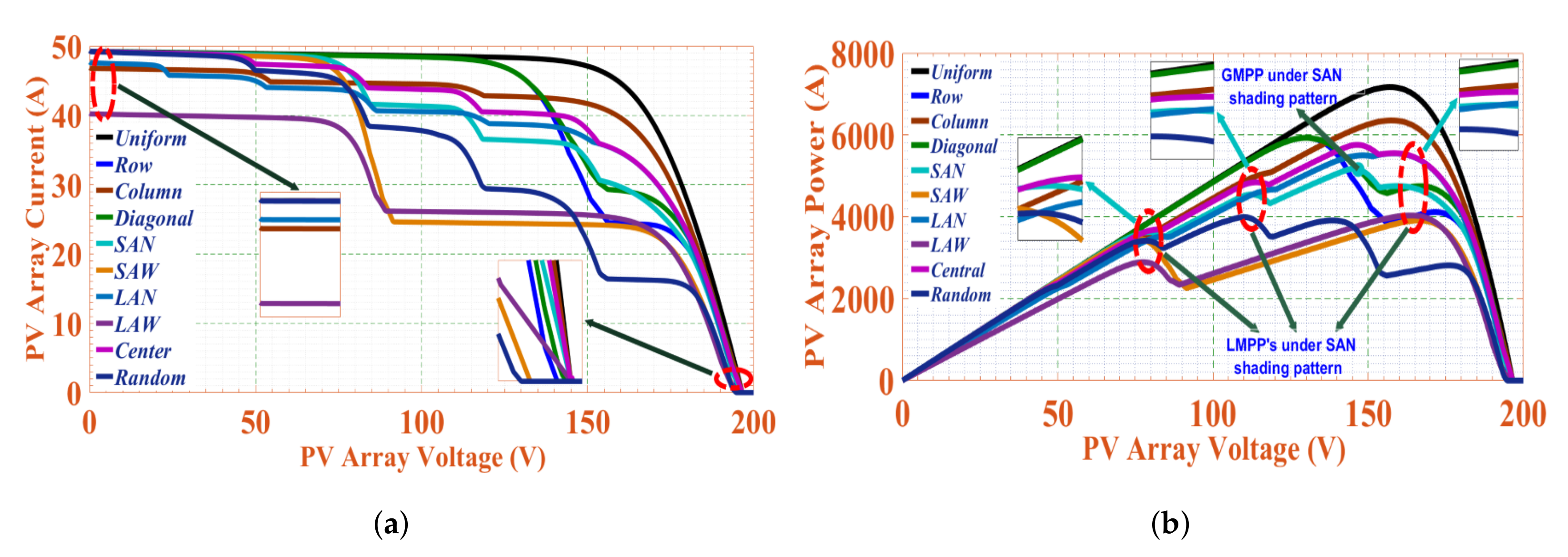
The performance of the S-P topology is superior to other topologies under the SAN shading pattern. The S-P topology generates GMPP at 5173.00 W. The corresponding and of an S-P topology at GMPP are 145.56 V and 35.53 A, respectively. The parameter variations of both the conventional and hybrid topologies are represented in Table 5. The S-P topology generates three number of LMPP’s, and their corresponding operating points are (3624.96 W, 79.51 V, 45.59 A), (4545.83 W, 112.47 V, 40.42 A) and (4751.67 W, 159.36 V, 29.82 A), respectively. The B-L, S-P-C-T, B-L-C-T, H-C-C-T, S-P-T-C-T, B-L-T-C-T, and H-C-T-C-T topologies also generate the same number of LMPP’s as that of the S-P topology. The B-L-H-C topology performance is lower compared to others, and it generates the GMPP at 4973.50 W. The corresponding and of a B-L-H-C topology at GMPP are 140.59 V and 35.37 A, respectively. The , , and of S-P topology under this shading pattern are 28.20%, 10.16% and 0.533, respectively. The calculated values of and of both the conventional and proposed hybrid topologies are represented in Figure 15d.
Table 5.
Parameter variations of conventional and hybrid array configurations under SAN pattern.
5.6. Under SAW Shading Pattern
The parameter variations of both the conventional and hybrid array topologies under the SAW shading pattern are represented in Table 6. Except for the S-P, all the PV array topologies generate the GMPP at 4480.25 W. The corresponding and of all the topologies except S-P are 105.24 V and 42.56 A, respectively. The S-P topology performance is lower than other topologies, and its operating points at GMPP are (3911.46 W, 166.34 V, 23.51 A). All PV array topologies except S-P represents two number of LMPP’s, whereas the S-P topology represents only one number of LMPP. The H-C-T-C-T topology operating points at LMPP’s are (3456.15 W, 75.97 V, 45.49 A) and (4056.55 W, 170.82 V, 23.75 A), respectively. The S-P topology operating points at LMPP are at (3455.96 W, 75.87 V, 45.54 A), respectively. The , , and of H-C-T-C-T topology under SAW shading pattern are 37.82%, 8.80% and 0.462, respectively. The calculated values of and of both the conventional and proposed hybrid topologies are represented in Figure 15e.
Table 6.
Parameter variations of conventional and hybrid configurations under SAW pattern.
5.7. Under LAN Shading Pattern
The calculated values of and of both the conventional and proposed hybrid topologies are represented in Figure 15f. The H-C-T-C-T topology generates the highest GMPP at 5863.35 W under the LAN shading pattern. The corresponding and of H-C-T-C-T topology at GMPP are 162.47 V and 36.08 A, respectively. The H-C-T-C-T topology represents five number of LMPP’s at an operating power, voltage and current of (854.86 W, 18.40 V, 46.46 A), (2031.24 W, 45.33 V, 44.81 A), (3161.04 W, 73.24 V, 43.16 A), (4318.02 W, 107.20 V, 40.28 A) and (5118.99 W, 133.90 V, 38.23 A), respectively. The B-L and B-L-T-C-T topologies also represent the five LMPP’s. The H-C, H-C-C-T, S-P-T-C-T, and B-L-H-C topologies represent three LMPP’s, whereas the S-P and S-P-T-C-T topologies represent four and two numbers of LMPP’s. The S-P topology performance is lower than other topologies, and its operating points at GMPP are (5549.50 W, 158.28 V, 35.06 A), respectively. The , , and of H-C-T-C-T topology under LAN shading pattern are 18.62%, 11.52%, and 0.604, respectively. The parameter variations of both conventional and hybrid topologies under the LAN shading pattern are represented in Table 7.
Table 7.
Parameter variations of conventional and hybrid array configurations under LAN pattern.
5.8. Under LAW Shading Pattern
The parameter variations of both the conventional and hybrid array topologies under the LAW shading pattern are represented in Table 8 and Figure 15g. The S-P-C-T, B-L-C-T, H-C-C-T, S-P-T-C-T, B-L-T-C-T, and H-C-T-C-T topologies under this shading pattern generate the same GMPP at 4140.75 W. The corresponding and of these topologies at GMPP are at 165.01 V and 25.09 A, respectively. The B-L-H-C topology performance is lower than other topologies, and its operating points at GMPP are (3823.80 W, 167.29 V, 22.86 A). All the PV array topologies except the B-L and B-L-H-C represent only one number of LMPP. The B-L and B-L-H-C topologies represent the two numbers of LMPP’s. The operating points of B-L topologies at LMPP’s are (2454.10 W, 93.50 V, 26.25 A) and (2843.10 W, 76.31 V, 37.25 A), whereas the B-L-H-C operating points at LMPP’s are (2454.10 W, 93.50 V, 26.25 A) and (3433.10 W, 139.34 V, 24.64 A), respectively. The H-C-T-C-T topology operating points at LMPP’s are (2843.10 W, 76.67 V, 37.07 A). The , and of H-C-T-C-T topology under this shading pattern is 42.53%, 8.13% and 0.427, respectively.
Table 8.
Parameter variations of conventional and hybrid configurations under LAW pattern.
5.9. Under Random Shading Pattern
The B-L-T-C-T topology generates the highest GMPP at 5218.25 W under a random shading pattern. The corresponding and of B-L-T-C-T topology at GMPP are 163.93 V and 31.83 A, respectively. The parameter variations of both the conventional and hybrid topologies under random shading patterns are represented in Table 9. The B-L-T-C-T topology represents three number of LMPP’s at an operating power, voltage, and current of (825.53 W, 20.13 V, 41.01 A), (2796.64 W, 72.19 V, 38.74 A) and (4692.15 W, 134.69 V, 34.84 A), respectively. The H-C-C-T, S-P-T-C-T, and H-C-T-C-T topologies also represent three LMPP’s. The B-L and H-C topologies represent five LMPP’s, whereas S-P, S-P-C-T, B-L-C-T, and B-L-H-C topologies represent the four LMPP’s. The S-P topology performance is lower than other topologies, and its operating points at GMPP are (3991.80 W, 110.06 V, 36.26 A). The , , and of B-L-T-C-T topology under this shading pattern are 27.58%, 10.25% and 0.538, respectively. The calculated values of and of both the conventional and proposed hybrid topologies are represented in Figure 15h.
Table 9.
Parameter variations of conventional and hybrid configurations under random pattern.
5.10. Under Center Shading Pattern
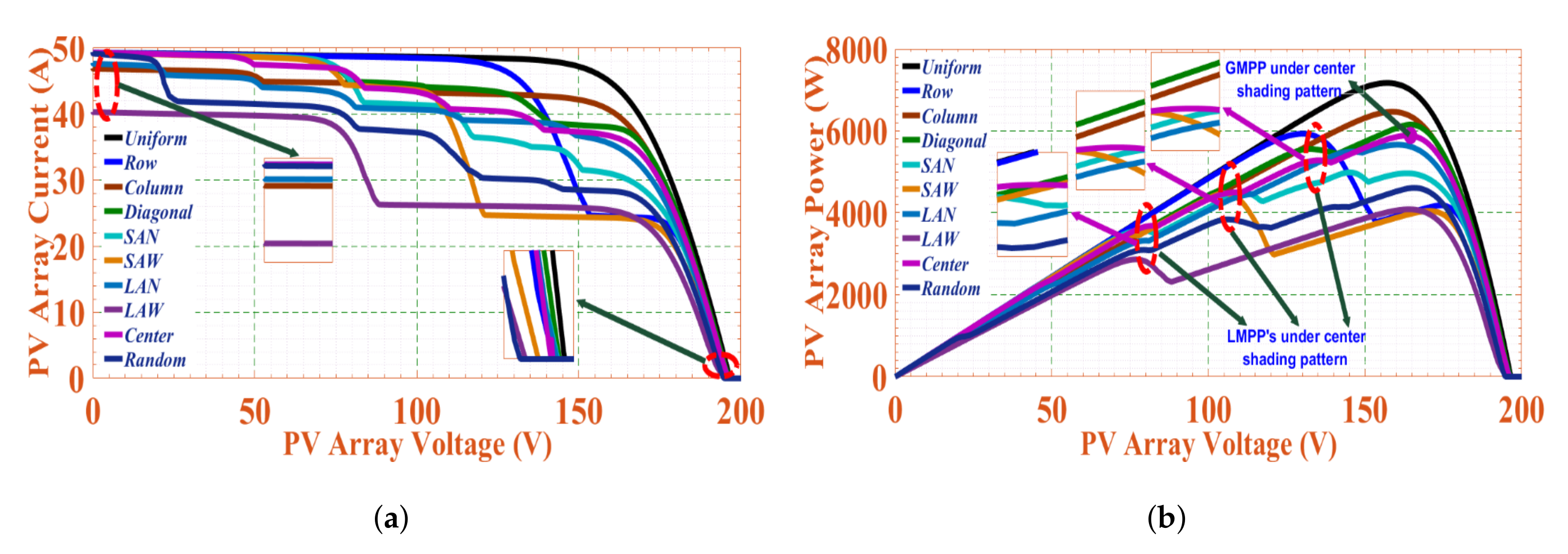
Under the center shading pattern, the performance of the H-C-T-C-T topology is superior over the other array topologies. The parameter variations of both the conventional and hybrid topologies under the center shading pattern are represented in Table 10. The calculated values of the and of both the conventional and proposed hybrid array topologies are represented in Figure 15i. The H-C-T-C-T topology generates the GMPP of 5906.25 W at and of 163.76 V and 36.06 A, respectively. The S-P, B-L, and H-C-T-C-T array topologies under the center shading pattern generate the four LMPP’s. The operating points of H-C-T-C-T topology at the four number of LMPP’s are (2082.73 W, 43.30 V, 48.10 A), (3386.77 W, 73.18 V, 46.28 A), (4459.08 W, 103.10 V, 43.25 A) and (5462.82 W, 136.40 V, 40.45 A), respectively. The H-C, S-P-C-T, B-L-C-T, S-P-T-C-T, B-L-T-C-T, and B-L-H-C array topologies generate the three number of LMPP’s, whereas the H-C-C-T topology generates only one number of LMPP. The B-L-H-C array topology performance is lower than other topologies, generating the GMPP at 5741.70 W. The corresponding and of B-L-H-C array topology at GMPP are 161.95 V and 35.45 A, respectively. The B-L-H-C array topology operating points at the LMPP’s are (3535.10 W, 79.20 V, 44.63 A), (4621.80 W, 108.68 V, 42.53 A) and (5601.4 W, 141.20 V, 39.67 A), respectively. The , and of H-C-T-C-T array topology under center shading pattern is 18.03%, 11.60% and 0.608, respectively.
Table 10.
Parameter variations of conventional and hybrid configurations under center shading pattern.
6. Conclusions
In this paper, we have proposed various hybrid PV array topologies such as S-P-C-T, B-L-C-T, H-C-C-T, S-P-T-C-T, B-L-T-C-T, H-C-T-C-T, and B-L-H-C to maximize the power output under PSCs. The different single diode PV module models, including their limitations, are also discussed. Mathematical modeling of PV module two-diode model in MATLAB/Simulink environment is also discussed. The proposed hybrid topologies have a lesser number of cross-tied connections over the T-C-T. Thus, the proposed hybrid topologies minimize the circuit wiring, wiring loss, and wiring cost. The proposed hybrid topology’s performance is evaluated and compared with the conventional array topologies such as S-P, B-L, and H-C under uneven-row, uneven-column, diagonal, SAN, SAW, LAN LAW, random and center shading patterns. The performance of the PV array topologies is evaluated by considering the variations in open-circuit voltage, short-circuit current, voltage and current at GMPP and LMPP’s, no. of peaks, fill factor, conversion efficiency, and mismatching power loss, respectively. The energy yield results prove that the H-C-T-C-T topology’s conversion efficiency and fill factor are higher at GMPP. Furthermore, the mismatching power loss is lower compared with the conventional and other proposed hybrid topologies. The H-C-T-C-T topology also reduces the number of LMPP’s under certain shading patterns compared to all other topologies. Hence, we concluded that the H-C-T-C-T topology is a suitable option for maximizing the power output under PSCs by reducing the mismatched power loss. These results provide valuable and reliable knowledge on the performance of PV array topologies under PSCs.
Author Contributions
Conceptualization—S.R.P. and S.M.; Methodology, Software, Validation—S.R.P., S.M., S.S.R., S.A., R.E.C. and T.S.; Investigation, Resources, Writing—Original Draft Preparation, Writing—Review and Editing, Visualization; Supervision; Project Administration, S.R.P., S.M., S.S.R., S.A., R.E.C. and T.S. All authors have read and agreed to the published version of the manuscript.
Funding
The authors gratefully acknowledge the support offered by the Science and Engineering Research Board (SERB), Department of Science and Technology, Government of India, under the Grant number: ECR/2017/000316 for this research work.
Conflicts of Interest
The authors declare no conflict of interest.
Nomenclature and Abbreviations
Nomenclature
| PV | Photovoltaic |
| S-S | Simple-Series |
| P | Parallel |
| S-P | Series-Parallel |
| T-C-T | Total-Cross-Tied |
| B-L | Bridge-Linked |
| H-C | Honey-Comb |
| S-P-C-T | Series-Parallel-Cross-Tied |
| B-L-C-T | Bridge-Linked-Cross-Tied |
| H-C-C-T | Honey-Comb-Cross-Tied |
| S-P-T-C-T | Series-Parallel-Total-Cross-Tied |
| B-L-T-C-T | Bridge-Linked-Total-Cross-Tied |
| H-C-T-C-T | Honey-Comb-Total-Cross-Tied |
| B-L-H-C | Bridge-Link-Honey-Comb |
| NUOC | Non-unioform Operating Condition |
| PID | Potential-Induced-Degradation |
| LMPP | Local-Maximum-Power-Point |
| GMPP | Global-Maximum-Power-Point |
| FF | Fill Factor |
Abbreviations
The following abbreviations are used in this manuscript:
| [A] | PV module output current |
| [A] | Photo-generated current |
| [A] | Photo-generated current at STC |
| [A] | PV module short-circuit current at STC |
| & [A] | Diode reverse saturation currents |
| [A] | PV array output current |
| [V] | PV module output voltage |
| & [V] | Thermal voltages of the diodes |
| [V] | PV module open-circuit voltage at STC |
| [V] | PV array output voltage |
| PV module series resistance | |
| PV module shunt resistance | |
| & [V] | Diffusion and recombination current components of the diodes |
| G [A] | Solar insolation at the particular level |
| [V] | Solar insolation at the STC |
| Temperature co-efficient of short-circuit current | |
| Temperature co-efficient of open-circuit voltage¶ |
References
- Villalva, M.G.; Gazoli, J.R.; Filho, E.R. Comprehensive approach to modeling and simulation of photovoltaic arrays. IEEE Trans. Power Electron. 2019, 24, 1198–1208. [Google Scholar] [CrossRef]
- Ding, K.; Bian, X.G.; Liu, H.H.; Peng, T. A MATLAB-Simulink-based PV module model and its application under conditions of nonuniform irradiance. IEEE Trans. Energy Convers. 2012, 27, 864–872. [Google Scholar] [CrossRef]
- Veerasamy, B.; Takeshita, T.; Jote, A.; Mekonnen, T. Mismatch loss analysis of PV array configurations under partial shading conditions. In Proceedings of the 7th IEEE International Conference on Renewable Energy Research and Applications (ICRERA), Paris, France, 14–17 October 2018; pp. 1162–1167. [Google Scholar]
- Krishna, G.S.; Moger, T. Comparative Study on Solar Photovoltaic Array Configurations Under Irregular Irradiance Conditions. In Proceedings of the 8th IEEE Intenational Conference on Power Electronics (IICPE), Jaipur, India, 13–15 December 2018; pp. 1–6. [Google Scholar]
- Moballegh, S.; Jiang, J. Modeling, prediction, and experimental validations of power peaks of PV arrays under partial shading conditions. IEEE Trans. Sustain. Energy 2014, 5, 293–300. [Google Scholar] [CrossRef]
- Ahmed, J.; Salam, Z. An accurate method for MPPT to detect the partial shading occurrence in a PV system. IEEE Trans. Ind. Inform. 2017, 13, 2151–2161. [Google Scholar] [CrossRef]
- Manganiello, P.; Balato, M.; Vitelli, M. A survey on mismatching and aging of PV modules: The closed loop. IEEE Trans. Ind. Electron. 2015, 62, 7276–7286. [Google Scholar] [CrossRef]
- Gao, L.; Dougal, R.A.; Liu, S.; Iotova, A.P. Parallel-connected solar PV system to address partial and rapidly fluctuating shadow conditions. IEEE Trans. Ind. Electron. 2009, 56, 1548–1556. [Google Scholar]
- Petrone, G.; Spagnuolo, G.; Teodorescu, R.; Veerachary, M.; Vitell, M. Reliability issues in photovoltaic power processing systems. IEEE Trans. Ind. Electron. 2008, 55, 2569–2580. [Google Scholar] [CrossRef]
- Patel, H.; Agarwal, V. MATLAB-based modeling to study the effects of partial shading on PV array characteristics. IEEE Trans. Energy Convers. 2008, 23, 302–310. [Google Scholar] [CrossRef]
- Wu, D.; Sun, Y.; Zheng, F. Research of a new photovoltaic module. Int. J. Energy Res. 2019, 43, 7702–7709. [Google Scholar] [CrossRef]
- Jazayeri, M.; Uysal, S.; Jazayeri, K. A comparative study on different photovoltaic array topologies under partial shading conditions. In Proceedings of the 2014 IEEE PES T&D Conference and Exposition, Chicago, IL, USA, 14–17 April 2014; pp. 1–5. [Google Scholar]
- Ramaprabha, R.; Mathur, B.L. A comprehensive review and analysis of solar photovoltaic array configurations under partial shaded conditions. Int. J. Photoenergy 2012, 2012, 1–16. [Google Scholar] [CrossRef] [Green Version]
- Killi, M.; Samanta, S. Modified perturb and observe MPPT algorithm for drift avoidance in photovoltaic systems. IEEE Trans. Ind. Electron. 2015, 62, 5549–5559. [Google Scholar] [CrossRef]
- Subudhi, B.; Pradhan, R. A comparative study on maximum power point tracking techniques for photovoltaic power systems. IEEE Trans. Sustain. Energy 2012, 4, 89–98. [Google Scholar] [CrossRef]
- Garud, K.S.; Jayaraj, S.; Lee, M.-Y. A review on modeling of solar photovoltaic systems using artificial neural networks, fuzzy logic, genetic algorithm and hybrid models. Int. J. Energy Res. 2021, 45, 6–35. [Google Scholar] [CrossRef]
- Salam, Z.; Ahmed, J.; Merugu, B.S. The application of soft computing methods for MPPT of PV system: A technological and status review. Appl. Energy 2013, 107, 135–148. [Google Scholar] [CrossRef]
- Bastidas-Rodriguez, J.D.; Franco, E.; Petrone, G.; Ramos-Paja, C.A.; Spagnuolo, G. Maximum power point tracking architectures for photovoltaic systems in mismatching conditions: A review. IET Power Electron. 2014, 7, 1396–1413. [Google Scholar] [CrossRef]
- Agamy, M.S.; Harfman-Todorovic, M.; Elasser, A.; Chi, S.; Steigerwald, R.L.; Sabate, J.A.; McCann, A.J.; Zhang, L.; Mueller, F.J. An Efficient Partial Power Processing DC/DC Converter for Distributed PV Architectures. IEEE Trans. Power Electron. 2014, 29, 674–686. [Google Scholar] [CrossRef]
- Pilawa-Podgurski, R.C.N.; Perreault, D.J. Sub-module integrated distributed maximum power point tracking for solar photovoltaic applications. IEEE Trans. Power Electron. 2013, 28, 2957–2967. [Google Scholar] [CrossRef] [Green Version]
- Pendem, S.R.; Mikkili, S.; Bonthagorla, P.K. PV distributed-MPP tracking: Total-cross-tied configuration of string-integrated-converters to extract the maximum power under various PSCs. IEEE Syst. J. 2019, 14, 1046–1057. [Google Scholar] [CrossRef]
- Kouro, S.; Leon, J.I.; Vinnikov, J.I.; Franquelo, L.G. Grid-connected photovoltaic systems: An overview of recent research and emerging PV converter technology. IEEE Ind. Electron. Mag. 2015, 9, 47–61. [Google Scholar] [CrossRef]
- Jalilzadeh, T.; Rostami, N.; Babaei, E.; Maalandish, M. Non-isolated topology for high step-up dc-dc converters. IEEE J. Emerg. Sel. Topics Power Electron. 2018, 1. [Google Scholar] [CrossRef]
- Li, W.; He, X. Review of nonisolated high-step-up dc/dc converters in photovoltaic grid-connected applications. IEEE Trans. Ind. Electron. 2011, 58, 1239–1250. [Google Scholar] [CrossRef]
- Al-Soeidat, M.; Aljarajreh, H.; Khawaldeh, H.; Lu, D.D.; Zhu, J.G. A reconfigurable three-port dc-dc converter for integrated PV-battery system. IEEE J. Emerg. Sel. Topics Power Electron. 2019, 8, 3423–3433. [Google Scholar] [CrossRef]
- Freitas, A.A.; Tofoli, F.L.L.; Mineiro, S.; Daher, S.; Antunes, F.M. High-voltage gain dc-dc boost converter with coupled inductors for photovoltaic systems. IET Power Electron. 2015, 8, 1885–1892. [Google Scholar] [CrossRef] [Green Version]
- Romero-Cadaval, E.; Spagnuolo, G.; Franquelo, L.G.; Ramos-Paja, C.-A.; Suntio, T.; Xiao, W.-M. Grid-connected photovoltaic generation plants: Components and operation. IEEE Ind. Electron. Mag. 2013, 7, 6–20. [Google Scholar] [CrossRef] [Green Version]
- Li, Q.; Wolfs, P. A review of the single phase photovoltaic module integrated converter topologies with three different dc link configurations. IEEE Trans. Power Electron. 2008, 23, 1320–1333. [Google Scholar]
- Gupta, K.K.; Ranjan, A.; Bhatnagar, P.; Sahu, L.K.; Jain, S. Multilevel inverter topologies with reduced device count: A review. IEEE Trans. Power Electron. 2016, 31, 135–151. [Google Scholar] [CrossRef]
- Hassaine, L.; OLias, E.; Quintero, J.; Salas, V. Overview of power inverter topologies and control structures for grid connected photovoltaic systems. Renew. Sustain. Energy Rev. 2014, 30, 796–807. [Google Scholar] [CrossRef]
- Moses, A.; Sun, H. Bidirectional energy storage photovoltaic grid-connected inverter application system. Int. J. Energy Res. 2020, 44, 11509–11523. [Google Scholar] [CrossRef]
- Alhafadhi, L.; Teh, J. Advances in reduction of total harmonic distortion in solar photovoltaic systems: A literature review. Int. J. Energy Res. 2020, 44, 2455–2470. [Google Scholar] [CrossRef]
- Khan, M.N.H.; Forouzesh, M.; Siwakoti, Y.P.; Li, L.; Kerekes, T.; Blaabjerg, F. Transformerless inverter topologies for single-phase photovoltaic systems: A comparative review. IEEE J. Emerg. Sel. Topics Power Electron. 2020, 8, 805–835. [Google Scholar] [CrossRef]
- Pendem, S.R.; Mikkili, S. Modelling and performance assessment of PV array topologies under partial shading conditions to mitigate the mismatching power losses. Sol. Energy 2018, 160, 303–321. [Google Scholar] [CrossRef]
- Gautam, N.K.; Kaushika, N. Reliability evaluation of solar photovoltaic arrays. Sol. Energy 2002, 72, 129–141. [Google Scholar] [CrossRef]
- Bosco, M.J.; Mabel, M.C. A novel cross diagonal view configuration of a PV system under partial shading condition. Sol. Energy 2017, 158, 760–773. [Google Scholar] [CrossRef]
- Bonthagorla, P.K.; Mikkili, S. A novel fixed PV array configuration for harvesting maximum power from shaded modules by reducing the number of cross-ties. IEEE J. Emerg. Sel. Topics Power Electron. 2020, 9, 2109–2121. [Google Scholar] [CrossRef]
- Lappalainen, K.; Valkealahti, S. Effects of irradiance transition characteristics on the mismatch losses of different electrical PV array configurations. IET Renew. Power Gener. 2016, 11, 248–254. [Google Scholar] [CrossRef]
- Rao, P.S.; Ilango, G.S.; Nagamani, C. Maximum power from PV arrays using a fixed configuration under different shading conditions. IEEE J. Photovoltaics 2014, 4, 679–686. [Google Scholar]
- Horoufiany, M.; Ghandehari, R. Optimal fixed reconfiguration scheme for PV arrays power enhancement under mutual shading conditions. IET Renew. Power Gener. 2017, 11, 1456–1463. [Google Scholar] [CrossRef]
- Sahu, H.S.; Nayak, S.K. Extraction of maximum power from a PV array under nonuniform irradiation conditions. IEEE Trans. Electron Devices 2016, 63, 4825–4831. [Google Scholar] [CrossRef]
- Rani, B.I.; Ilango, G.S.; Nagamani, C. Enhanced power generation from PV array under partial shading conditions by shade dispersion using Su Do Ku configuration. IEEE Trans. Sustain. Energy 2013, 4, 594–601. [Google Scholar] [CrossRef]
- Krishna, S.G.; Moger, T. Optimal SuDoKu reconfiguration technique for total-cross-tied PV array to increase power output under non-uniform irradiance. IEEE Trans. Energy Convers. 2019, 34, 1973–1984. [Google Scholar] [CrossRef]
- Yadav, A.S.; Pachauri, R.K.; Chauhan, Y.K. Comprehensive Investigation of PV arrays with puzzle shade dispersion for improved performance. Sol. Energy. 2016, 129, 256–285. [Google Scholar] [CrossRef]
- Vijayalekshmy, S.; Bindu, G.R.; Iyer, S.R. A novel zig-zag scheme for power enhancement of partially shaded solar arrays. Sol. Energy 2016, 135, 92–102. [Google Scholar] [CrossRef]
- Dhanalakshmi, B.; Rajasekar, N. Dominance square based array reconfiguration scheme for power loss reduction in solar PhotoVoltaic (PV) systems. Energy Convers. Manag. 2015, 156, 84–102. [Google Scholar] [CrossRef]
- Rakesh, N.; Kumar, S.S.; Madhusudanan, G. Mitigation of power mismatch losses and wiring line losses of partially shaded solar PV array using improvised magic technique. IET Renew. Power Gener. 2019, 13, 1522–1532. [Google Scholar] [CrossRef]
- Nguyen, D.; Lehman, B. An adaptive solar photovoltaic array using model-based reconfiguration algorithm. IEEE Trans. Ind. Electron. 2008, 55, 2644–2654. [Google Scholar] [CrossRef]
- Velasco-Quesada, G.; Guinjoan-Gispert, F.; Pique-Lopez, R.; Roman-Lumbreras, M.; Conesa-Roca, A. Electrical PV array reconfiguration strategy for energy extraction improvement in grid-connected PV systems. IEEE Trans. Ind. Electron. 2009, 56, 4319–4331. [Google Scholar] [CrossRef] [Green Version]
- Deshkar, S.N.; Dhale, S.B.; Mukherjee, J.S.; Babu, T.S.; Rajasekar, N. Solar PV array reconfiguration under partial shading conditions for maximum power extraction using genetic algorithm. Renew. Sustain. Energy Rev. 2015, 43, 102–110. [Google Scholar] [CrossRef]
- Babu, T.S.; Prasanth Ram, J.; Dragicevic, T.; Miyatake, M.; Blaabjerg, F.; Rajasekar, N. Particle swarm optimization based solar PV array reconfiguration of the maximum power extraction under partial shading conditions. IEEE Trans. Sustain. Energy 2018, 9, 74–85. [Google Scholar] [CrossRef]
- Manjunath, M.; Reddy, B.V.; Lehman, B. Performance improvement of dynamic PV array under partial shade conditions using M2 algorithm. IET Renew. Power Gener. 2019, 13, 1239–1249. [Google Scholar] [CrossRef]
- Balato, M.; Manganiello, P.; Vitelli, M. Fast dynamical reconfiguration algorithm of PV arrays. In Proceedings of the 9th IEEE International Conference on Ecological Vehicles and Renewable Energies (EVER), Monte-Carlo, Monaco, 25–27 March 2014; pp. 1–8. [Google Scholar]
- Balato, M.; Costanzo, L.; Vitelli, M. Multi-objective optimization of PV arrays performances by means of the dynamical reconfiguration of PV modules connections. In Proceedings of the 2015 IEEE International Conference on Renewable Energy Research and Applications (ICRERA), Palermo, Italy, 22–25 November 2015; pp. 1646–1650. [Google Scholar]
- Storey, J.P.; Wilson, P.R.; Bagnall, D. Improved Optimization Strategy for Irradiance Equalization in Dynamic Photovoltaic Arrays. IEEE Trans. Power Electron. 2013, 28, 2946–2956. [Google Scholar] [CrossRef]
- Aldaoudeyeh, A.M.I. Photovoltaic-battery scheme to enhance PV array characteristics in partial shading conditions. IET Renew. Power Gener. 2016, 10, 108–115. [Google Scholar] [CrossRef]
- Sharma, P.; Agarwal, V. Maximum power extraction from a partially shaded PV array using shunt-series compensation. IEEE J. Photovoltaics 2014, 4, 1128–1137. [Google Scholar] [CrossRef]
- Pendem, S.R.; Mikkili, S. Modeling, simulation, and performance analysis of PV array configurations (series, series-parallel, bridge-linked, and honey-comb) to harvest maximum power under various partial shading conditions. Int. J. Green Energy 2018, 15, 795–812. [Google Scholar] [CrossRef]
- Shongwe, S.; Hanif, M. Comparative analysis of different single-diode PV modeling methods. IEEE J. Photovoltaics 2015, 5, 938–946. [Google Scholar] [CrossRef]
- Ma, J.; Man, K.; Guan, S.-U.; Ting, T.; Wong, P. Parameter estimation of photovoltaic model via parallel particle swarm optimization algorithm. Int. J. Energy Res. 2015, 40, 343–352. [Google Scholar] [CrossRef]
- Ishaque, K.; Salam, Z.; Taheri, H. Accurate MATLAB Simulink pv system simulator based on a two-diode model. Jour. Power Electron. 2011, 11, 17–187. [Google Scholar] [CrossRef] [Green Version]
- Villalva, M.G.; Gazoli, J.R.; Filho, E.R. Modeling and circuit-based simulation of photovoltaic arrays. In Proceedings of the 2009 Brazilian Power Electronics Conference (COBEP), Bonito-Mato Grosso do Sul, Brazil, 27 September–1 October 2009; pp. 1244–1254. [Google Scholar]
- Agrawal, N.; Bora, B.; Kapoor, A. Experimental investigations of fault tolerance due to shading in photovoltaic modules with different interconnected solar cell networks. Sol. Energy 2020, 211, 1239–1254. [Google Scholar] [CrossRef]
- Rao, P.S.; Dinesh, P.; Ilango, G.S.; Nagamani, C. Optimal Su-Do-Ku based interconnection scheme for increased power output from PV array under partial shading conditions. Front. Energy 2015, 9, 199–210. [Google Scholar]


Publisher’s Note: MDPI stays neutral with regard to jurisdictional claims in published maps and institutional affiliations. |
© 2021 by the authors. Licensee MDPI, Basel, Switzerland. This article is an open access article distributed under the terms and conditions of the Creative Commons Attribution (CC BY) license (https://creativecommons.org/licenses/by/4.0/).