Abstract
Power-domain non-orthogonal multiple access (NOMA) assigns different power levels for near and far users in order to discriminate their signals by employing successive interference cancellation (SIC) at the near user. In this context, multiple-input-single-output NOMA (MISO-NOMA), where the base station (BS) is equipped with multiple antennas while each mobile user has a single antenna receiver, is shown to have a better overall performance by using the knowledge of instantaneous channel state information (CSI). However, this requires prior estimation of CSI using pilot transmission, which increases the transmission overhead. Moreover, its performance is severely degraded in the presence of CSI estimation errors. In this work, we provide statistical beamforming solutions for downlink power-domain NOMA that utilize only knowledge of statistical CSI, thus reducing the transmission overhead significantly. First, we derive the outage probabilities for both near and far users in the multi-user NOMA system without imposing strong assumptions, such as Gaussian or Chi-square distribution. This is done by employing the exact characterization of the ratio of indefinite quadratic form (IQF). Second, this work proposes two techniques to obtain the optimal solution for beam vectors which rely on the derived outage probabilities. Specifically, these two methods are based on (1) minimization of total beam power while constraining the outage probabilities to the QoS threshold, and (2) minimization of outage probabilities while constraining the total beam power. These proposed methods are non-convex function of beam vectors and, hence, are solved using numerical optimization via sequential quadratic programming (SQP). Since the proposed methods do not require pilot transmission for channel estimation, they inherit better spectral efficiency. Our results validate the theoretical findings and prove the supremacy of the proposed method.
1. Introduction
Non-orthogonal multiple access (NOMA) constitutes a spectrum-efficient solution that can accommodate the huge data traffic of 5G networks [1,2]. NOMA techniques are typically integrated with other schemes, such as millimeter wave, beamforming and massive MIMO [3]. In contrast to the classical orthogonal multiple access (OMA) techniques, such as frequency division multiple access, NOMA has the capability of serving multiple users using the same (time, frequency, and code) resource blocks. This can be attained, in power-domain NOMA, by superimposing users’ streams into one signal while employing the successive interference cancellation (SIC) at the receivers [1,4,5]. The strong user, also known as the near user, decodes the weak user signal first and then decodes its own. Only a small amount of power has to be allocated to the strong user to give it a high rate while delivering near-optimal performance to the weak user [4,5].
Motivated by the spectral efficiency enhancement provided by NOMA schemes, several combined NOMA-aided beamforming multiple-input multiple-output (MIMO) schemes have been proposed recently [1,4,6,7,8,9]. However, designing efficient combined schemes includes several challenges, such as power allocations, user coordination, physical layer security and user clustering/selection [2,4]. For example, in [1], a joint user selection with optimized beamforming scheme was proposed for mmWave communication. Additionally, a combined game-based user clustering strategy and optimized beamforming techniques were suggested in [4]. Similarly, NOMA power allocation using the Glicksberg game was proposed in [6]. In [8], the beamforming optimization was carried out using the instantaneous channel state information (CSI). In [9], a scheme for joint beamforming and artificial noise optimization for MISO-NOMA cognitive radio was proposed that promises improved physical layer security. Meanwhile, the works in [10,11,12] addressed various issues in SIC for power domain NOMA.
The work in [13] discussed why and when NOMA is inefficient in multi-antenna settings by comparing its performance with multi-user linear precoding (MU–LP) and rate-splitting multiple access (RSMA). Although this work provides theoretical and numerical proofs for the inefficiency of NOMA in a multi-antenna scenario, these proofs are valid for specific scenarios. For example, MISO NOMA (here, G stands for the number of users in NOMA user groups, while M and K denote the number of antenna elements and total number of users, respectively) with and can outperform or achieve the same performance as MU–LP when in terms of max-min fair (MMF) multiplexing gain and has inferior performance for . Thus, MISO NOMA is still efficient for . Similarly, their numerical results provided in Figures 10 and 11 of [13] for sum rate and MMF, respectively, show that the performance of MISO NOMA has inferior performance than that of the RS only in the case of larger SNR values. On the other hand, their performance is almost identical for low SNR values. Thus, the utilization of MISO NOMA is still applicable for practical scenarios where SNR values are small. Finally, all the comparisons made in [13] are based on sum rate and MMF only. Moreover, their work is based on CSI estimation (whether perfect or imperfect), which requires pilot transmission. In contrast, we propose a blind technique without requiring any pilot transmission.
In contrast to the pilot-based approaches, we propose statistical beamforming solutions for the downlink power-domain NOMA which do not require CSI estimation, thereby reducing the transmission overhead, which eventually enhances the spectral efficiency. For this purpose, closed form expression for the outage probabilities for both near and far users in the NOMA system is derived using the characterization of IQF [14]. The optimum beam vectors are then obtained by two approaches: (1) by minimizing the total beam power while constraining the outage probabilities to the QoS threshold, and (2) by minimizing the outage probabilities while constraining the total beam power. Thus, our proposed system can be used for low-latency communication in MTC (thanks to the no-CSI feedback as well as a low outage probability).
Paper Contributions
Main contributions of our work can be summarized as follows:
- (a)
- Unlike the existing works which employ approximate characterization to derive outage probabilities, such as Gaussian or Chi-square distribution assumption, this work derives closed form expression for the outage probabilities for both near and far users in the multi-user NOMA system without imposing such assumptions. To elaborate further, we use the exact characterization of the ratio of IQF of the form (the notation represents the weighted norm defined as ) where is a scalar quantity, is a complex circular Gaussian vector, and and are certain weighting matrices.
- (b)
- This work proposes two techniques to obtain an optimal solution for beam vectors which rely on the derived outage probabilities. More precisely, these techniques are as follows:
- (i)
- To obtain the optimal beam vectors by minimizing the total beam power while constraining the outage probabilities to the QoS threshold.
- (ii)
- To obtain the optimal beam vectors by minimizing the outage probabilities while constraining the total beam power.
The propose methods (i) and (ii) are non-convex function of beam vectors. Thus, we implement numerical optimization method of SQP [15,16,17] by evaluating the gradients of the proposed objective function. - (c)
- It is important to highlight that the proposed methods require only statistical CSI in contrast to the existing works in [5,18], which employ the knowledge of instantaneous CSI. Thus, the proposed methods do not require pilot transmission for channel estimation and hence, can provide better spectral efficiency in contrast to the existing methods, which need pilot transmission.
2. Materials and Methods
2.1. System Model
Without loss of generality, we consider a cellular-based downlink multiuser transmission of Figure 1 in which the M-element antenna array-aided base station (BS) will transmit its signal to two users, each equipped with a single antenna [1,18]. Moreover, we have considered that there are total K users that are grouped into number of pairs, where each pair consists of a near user and a far user.
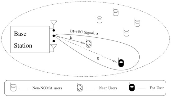
Figure 1.
The downlink beamforming plus superposition code (BF + SC) system model transmission.
The near user from the BS is denoted as , while the far user, also known as a cell-edge user, is denoted as . Both user signals are superposed using the superposition coding (SC) technique, then transmitted using an optimized beamforming (BF) scheme. Hence, the BS in our NOMA system is capable of serving multiple users simultaneously. Now, consider the pair whose BS (BF + SC) transmitted signal can be written as follows:
where and are near and far user signals in the pair, respectively, and and represent, respectively, the beamforming vectors for near and far users in the pair. Thus, the total broadcast signal for the L pairs will be
With the aid of Figure 1, the received signals at both and for the pair are given, respectively, by the following:
where and are channel vectors for the near and far users, respectively, in the pair. These vectors are assumed to be frequency-flat block fading channels. Moreover, and are the zero mean additive white Gaussian noises (AWGN)s for the near and the far users, respectively, i.e., and .
In the NOMA system, where generally , it can be thus assumed that the near user can decode both the near and far users’ data streams of their own pair. However, the far user needs only to decode their pair transmitted sequence. The power allocated to the beam vector of is typically lower than the counterpart, i.e., [7,18]. Thus, at the near user, SIC is employed to completely remove all the far user’s data from the superimposed received signal. As a result, the near user’s signal is decoded using SINR (denoted by ), while the far user is decoded using SINR (denoted by ). Now, using Equations (3) and (4), the and can be expressed as follows:
At the far user, the (from all pairs) and the (from all pairs excluding the pair) are considered interference terms but these may not be decoded, as their signal powers are severely faded [5,18]. Therefore, the SINR (denoted by ) for is given by the following:
2.2. Derivation of Outage Probabilities
In this section, we derive the outage probabilities for , , and . To do so, we employ a generic framework that can incorporate all the aforementioned SINRs. First, we reformulate the , , and defined in (5) and (6) as follows:
and
By observing the required SINRs in (7)–(9), it can be concluded that all the required SINRs can be dealt by defining the following generic variables:
where is a complex circular Gaussian vector such that , and are the matrices formed by product of beam vectors, and is the noise variance with subscript i in the set . It can be easily seen that the variable Y can incorporate all SINRs defined in Equations (7)–(9) with the proper choice of variables , , and (e.g., can be either or , and can be any of the weighting matrices formed by the beam vectors and/or ).
Next, following the approach of [19], the variable Y can be expressed as a ratio of indefinite quadratic forms as follows:
where is the whitened version of , while the matrices and are defined as
Now, using the definition of outage probability, the outage probability of Y (denoted by ) for any given threshold value can be formulated as follows:
The solution of the above probability can be found using the approach outlined in [19] which results in the following:
where represents the unit step function and is the eigenvalue of the matrix .
2.3. Design of Optimized Beamvectors for the NOMA System
In this section, we provide two schemes to design optimal multicast beamforming with SC for the NOMA system. These methods are based on statistical performance measures, that is, the outage probability of near and far users which relies only on the channel statistics in terms of eigenvalues of the channel correlation matrix.
2.3.1. Task 1: Beam Power Minimization While Constraining the Outage Probabilities
The task of optimal multicast beamforming with SC is to minimize the total power for beam vectors while achieving reliable signal reception. It should be noted that the eigenvalues appearing in Equation (14) are the function of beam vectors and . Thus, we can design optimal beam vectors by minimizing the total beam powers while constraining the outage probability at the near user and the worst outage probability at the far user [5,18]. To do so, we formulate the optimization problem as the minimum power multicast beamforming as follows:
The first constraint in the above is employed to meet the requirement of power-domain NOMA. The second constraint is forcing the outage of the near user at the near user receiver to be less than the selected maximum acceptable value (the value of the maximum acceptable outage is usually determined by the QoS requirements) (denoted by ) which is required to successfully decode the signal after SIC at the near user receiver. Finally, the last constraint is utilized to limit the worst case outage of the far user to be less than a certain maximum acceptable value (denoted by ) which makes sure that the signal can be successfully decoded at both the near and far users. The objective function of Equation (15) is a non-convex function of beam vectors whose unique solution cannot be obtained. Thus, we employ numerical optimization methods, such as active set (AS) optimization and SQP [15,16,17] to solve the above optimization task. An overview of the SQP optimization is provided in Appendix A while the evaluation of required gradients in our optimization tasks is provided in Appendix B.
Remark 1.
In contrast to the optimization problem defined in [5,18], where the constraints were applied to instantaneous SINRs (which assumes that the knowledge of instantaneous channels for both near and far users are available), we applied constraints on the outage probabilities, which only requires the statistics of the channel [14,19]. Thus, the proposed optimization problem is trying to find the optimal beam vectors by utilizing only the knowledge of channel statistics with much lesser computational complexity and bandwidth requirements than the one required for instantaneous channel information-based beamforming.
2.3.2. Task 2: Outage Probabilities Minimization While Constraining the Transmit Beam Powers
In this task, we propose to design optimum beam vectors by minimizing the sum outage probabilities while constraining the total beam power to unity. The sum outage probability is defined as follows:
where the factor of is used to normalize the maximum total probability to unity. Next, we propose the beamforming design via the following optimization task:
The first constraint in the above is employed to meet the requirement of power-domain NOMA. The second constraint is used to limit the total power to unity. Again, the objective function of Equation (17) is a non-convex function, and the numerical optimization method of AS and SQP are employed to find its solution. The implementation of these methods can be done using the approach outlined in Appendices Appendix A and Appendix B.
The pseudo-code for the the beamforming optimization in NOMA using Task 1 and Task 2 can be summarized in Algorithm 1 as follows:
| Algorithm 1 NOMA-BeamformingOptimization Algorithm. |
|
3. Results and Discussion
In this section, we report the results for our proposed multicast beamforming NOMA systems. Note that our proposed solution is valid for any number of users in NOMA systems. However, we present the results for two users only to show the proof of concept. We use and in our simulations. We set the length of beam vectors to , and the additive noise variance is such that the SNR is kept to 20 dB. The channel vectors are generated as complex zero-mean circular Gaussian random vectors with a correlation matrix with exponential correlation coefficients, i.e., (the correlation coefficient lies in [0, 1]). To implement the power domain NOMA, we set the beam vectors as follows:
where . The SC powers assigned to near and far users are 0.2 and 0.8, respectively (i.e., and ), where the summation of the two powers is normalized for fair comparison.
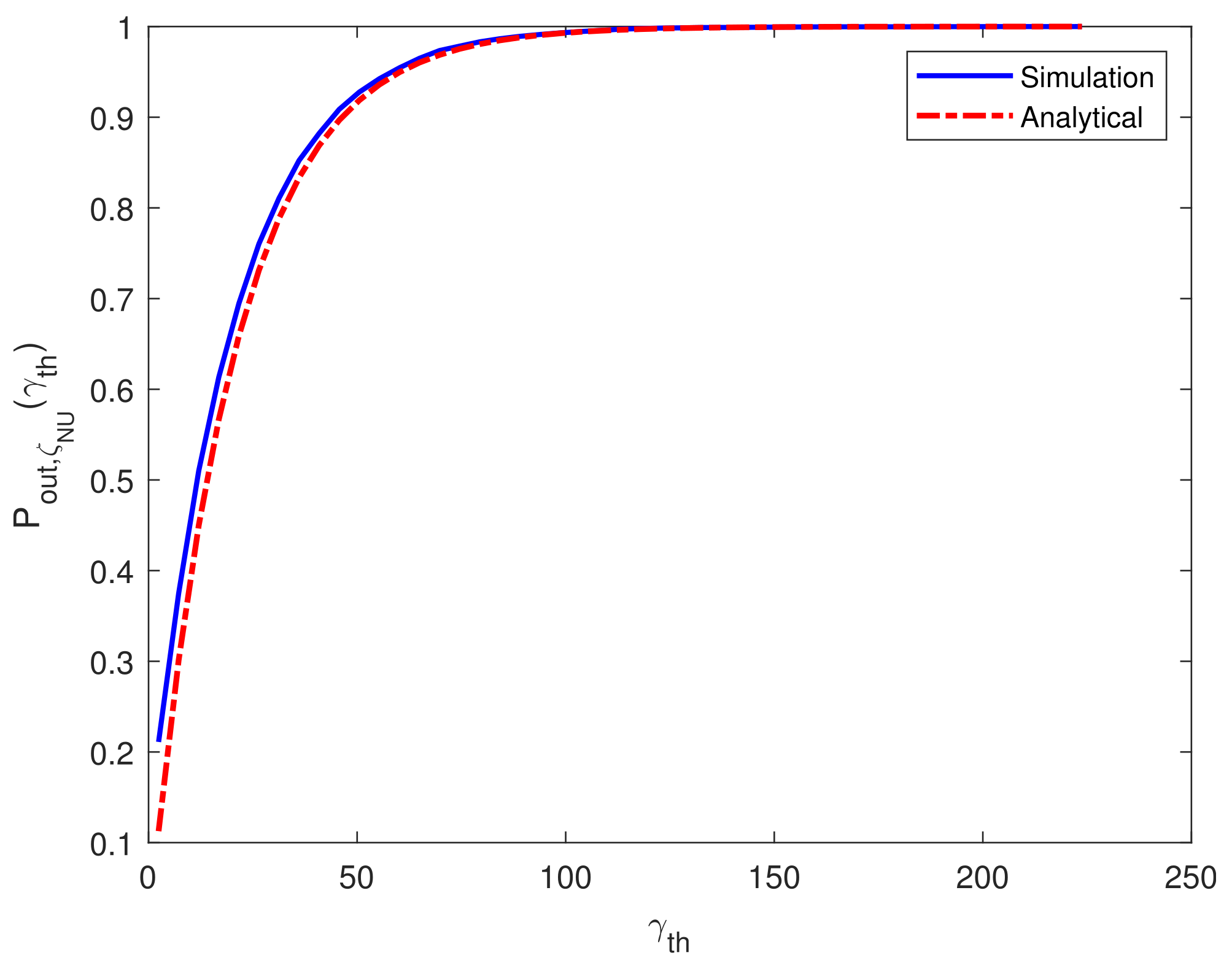
First of all, we validate the derived analytical expression of outage probability for in Figure 2 by comparing the Monte Carlo simulation results with the one obtained via the analytical expression in Equation (14) with eigenvalues calculated from the matrix and setting . It can be depicted from Figure 2 that there is a good match between the simulation and the derived analytical expression.
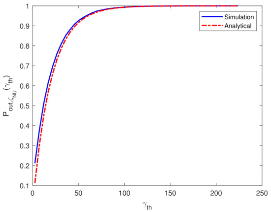
Figure 2.
Validation of analytical outage probability for .
3.1. Results for Task 1
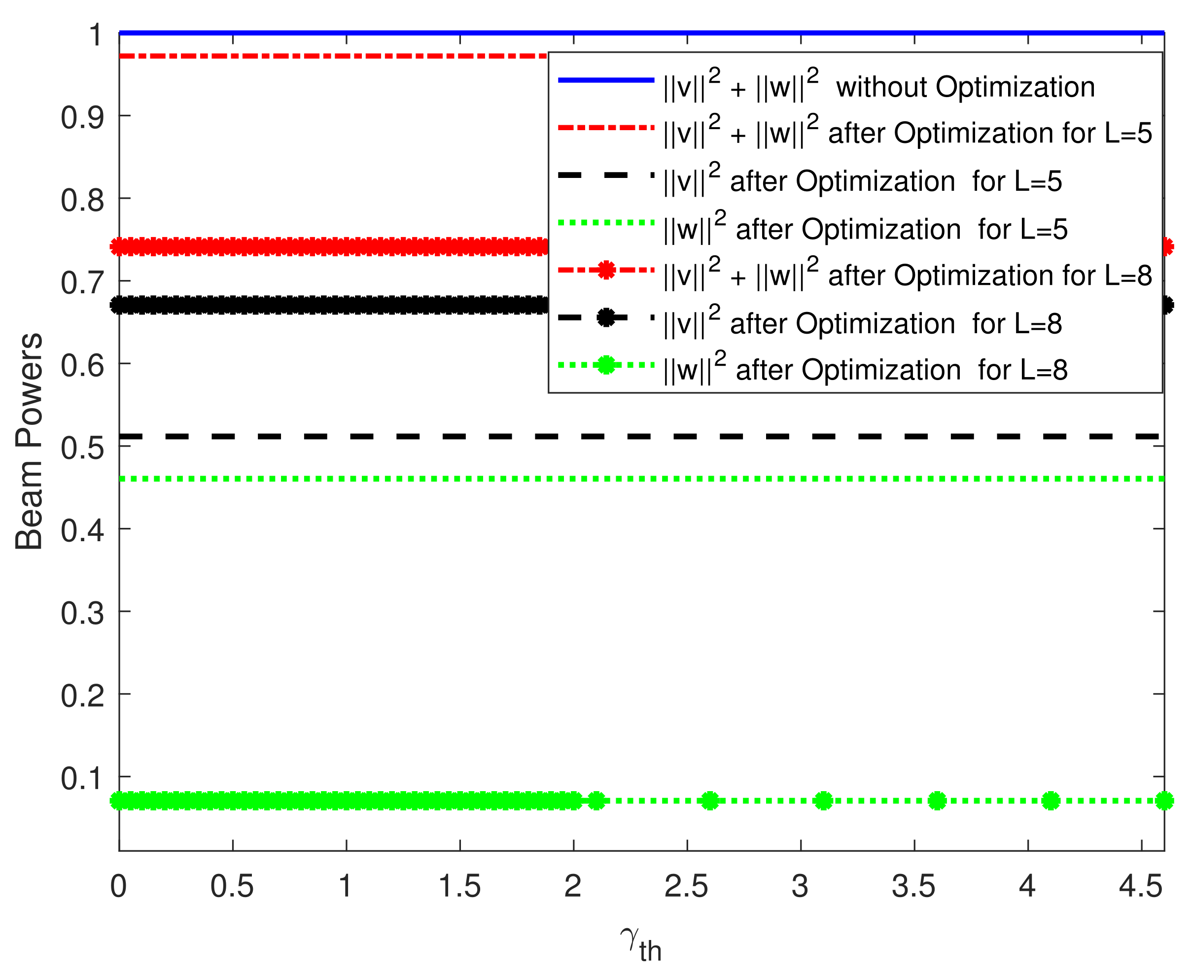
In this part, we investigate the performance of the beamforming optimization via Equation (15). The results in Figure 3 illustrate the optimization performance for beam powers , , and for two different lengths of antenna array, that is, and . It can be seen that the total beam power is minimized in both scenarios while the constraint on individual powers, that is, is also satisfied. Moreover, it can be observed that the power minimization is more for in contrast to , showing the benefit of using a larger antenna array. Next, in Figure 4, the performance of the outage probability constraint for is investigated for , which clearly exhibits a reduction in outage probability, thereby satisfying the constraint successfully.

Figure 3.
Optimization performance for beam powers with and .
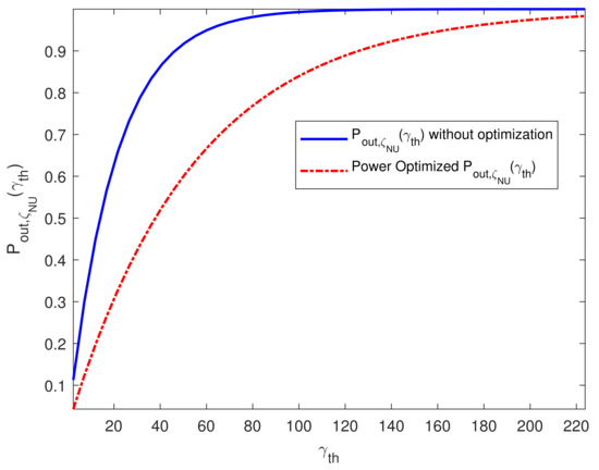
Figure 4.
Performance of outage probability constraint for for .
Next, in Figure 5, the performance of the outage probability constraint for the far user is compared before and after optimization. It can be depicted from the figure that the worst outage probability of the far user never exceeds the limit and hence, successfully meets the desired constraint. Moreover, it can be easily seen that the proposed method not only satisfies the constraints, but also minimizes the outage probability w.r.t. to the constraint reference. Hence, the overall performance of the proposed beamforming method can achieve both lower transmission power as well as lower outage probabilities for both near and far users, which guarantee reliable QoS service. It should not be forgotten that the proposed method is bandwidth efficient, as it does not require to send pilots for channel estimation.
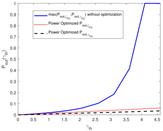
Figure 5.
Performance of outage probability constraint for far user.
3.2. Results for Task 2
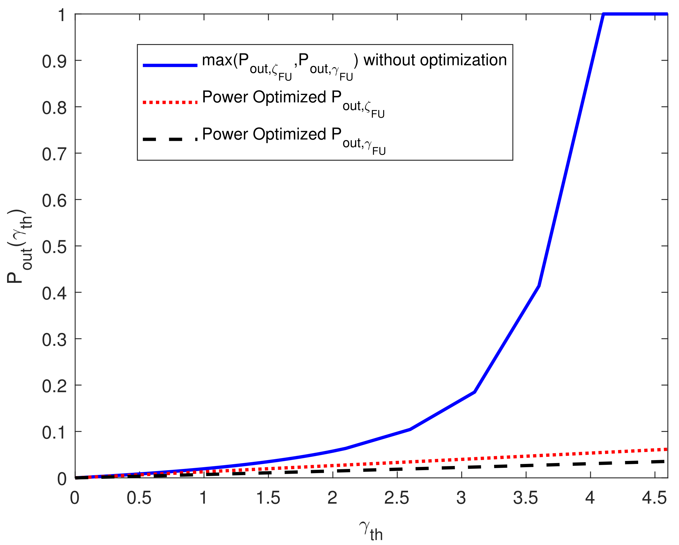
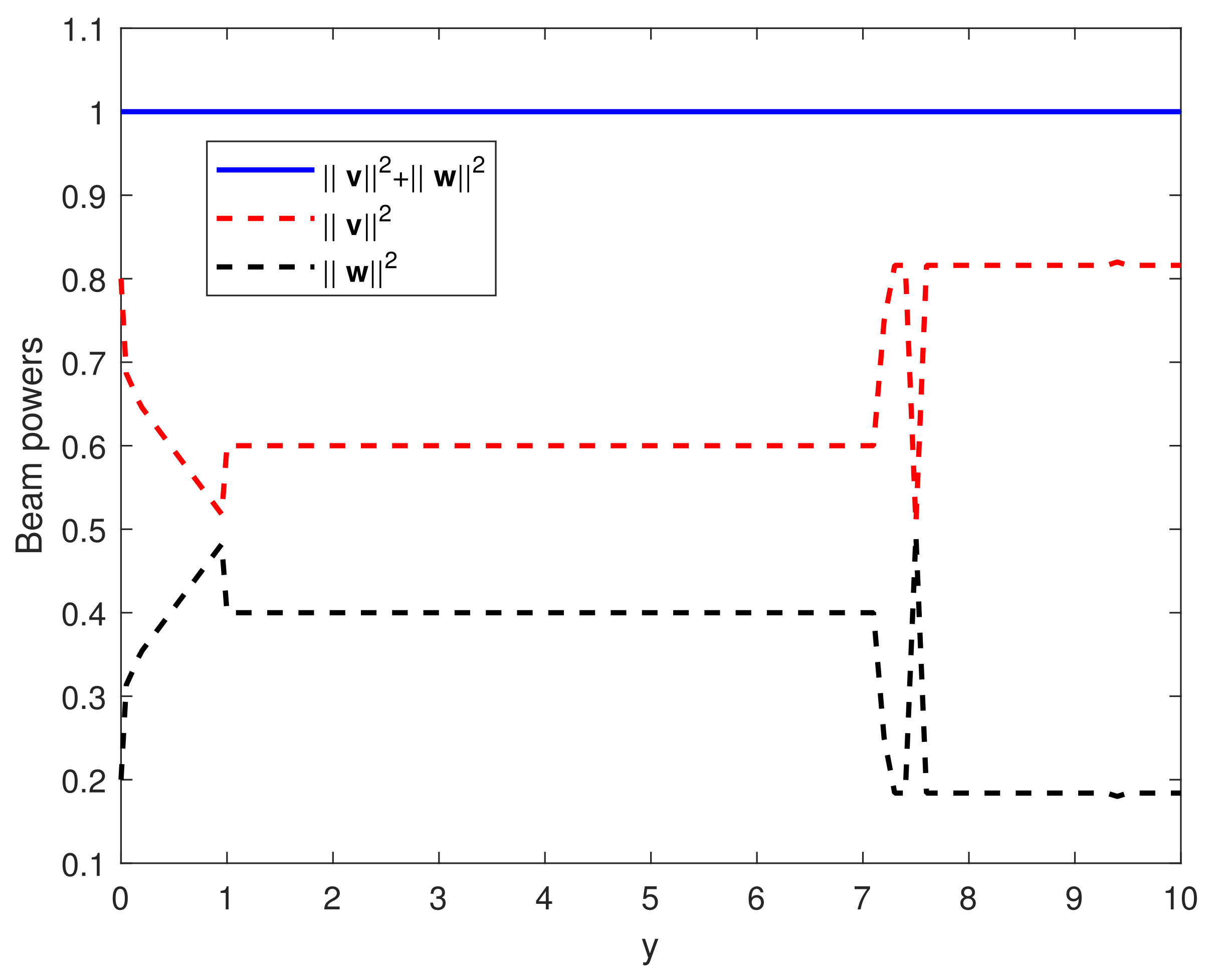
Next, we demonstrate the performance of the beamforming optimization via Equation (17). In Figure 6, the total outage probability is plotted before and after optimization by minimizing the objective function in (17) via the AS method. It can be observed that the proposed method can achieve a remarkable reduction in the total outage probability. On the other hand, the result in Figure 7 shows that the constraints on the beam power employed in (17) are satisfied for the whole range of . Thus, the beam vectors obtained via (17) maintain the total beam power to unity (i.e., ) while the beam power of the far user is greater than the that of the near user (i.e., ).
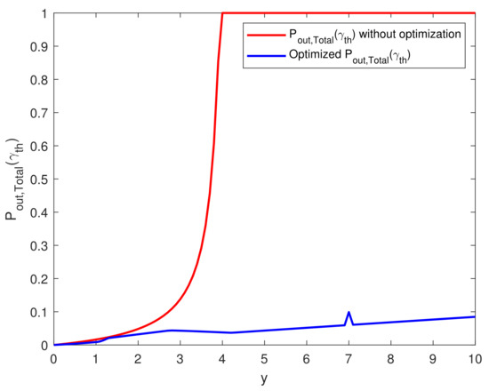
Figure 6.
Performance of outage probability minimization via Task 2.
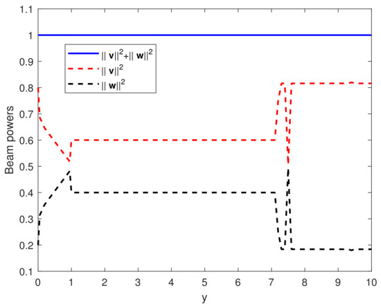
Figure 7.
Beam powers after optimization via Task 2.
4. Conclusions
In this work, we proposed spectral efficient beamforming schemes for downlink power-domain NOMA, as it does not require pilots transmission for channel estimation. In the proposed methods, the beam vectors are optimized using two approaches:
- By minimizing the total beam powers while constraining the outage probabilities for near and far users;
- By minimizing the total outage probabilities in the system while constraining the beam powers.
To achieve this, outage probabilities derived in a closed form, which, in turn, were utilized to implement the desired optimization tasks via the AS and SQP methods. The performance of the proposed algorithms was tested for different scenarios, showing that the proposed beamforming method can provide both lower transmission power as well as lower outage probabilities for both near and far users. Most importantly, the proposed schemes rely only on the statistical CSI, which reduces the transmission overhead. Thus, our proposed system can be considered a strong candidate for spectral efficient 5G communications.
Author Contributions
Conceptualization, A.J.A. and M.M.; methodology, A.J.A. and M.M.; software, A.J.A. and M.M.;validation, A.J.A. and M.M.; formal analysis, A.J.A. and M.M.; investigation, A.J.A. and M.M.; resources, A.J.A. and M.M.; data curation, A.J.A. and M.M.; writing—original draft preparation, A.J.A. and M.M.; writing—review and editing, A.J.A. and M.M.; visualization, A.J.A. and M.M.; supervision, M.M.; project administration, A.J.A.; funding acquisition, A.J.A. All authors have read and agreed to the published version of the manuscript.
Funding
This Project was funded by the Deanship of Scientific Research (DSR) at King Abdulaziz University, Jeddah, under grant no. (J:60-135-1441). The author, therefore, acknowledge with thanks the DSR for technical and financial support.
Acknowledgments
This project was funded by the Deanship of Scientific Research (DSR) at King Abdulaziz University, Jeddah, under grant no. (J:60-135-1441). The author, therefore, acknowledges, with thanks, the DSR for technical and financial support.
Conflicts of Interest
The authors declare no conflict of interest.
Appendix A. Overview of Sequential Quadratic Programming
In this Appendix, we provide an overview of the SQP optimization that can be used to solve any nonlinear optimization problem of the following form:
where , , and are objective function, equality constraints, and inequality constraints, respectively. The SQP is an iterative optimization technique which models the non-linear optimization problem in (A1) at iteration k (i.e., ) by a quadratic programming (QP) sub-problem. Next, it solves that QP sub-problem to obtain the solution for iteration (i.e., ), which results in a local minimum of the actual objective function. The Lagrangian functional for the problem in (A1) can be formulated as follows:
where and are the Lagrangian multipliers for equality and inequality constraints, respectively. In order to solve the above problem, the SQP utilizes the following QP sub-problem formation:
where and ▽ represents the gradient operation. The Hessian matrix appeared in the above can be calculated using the Broyden–Fletcher–Goldfarb–Shanno (BFGS) method [20,21,22,23]. Finally, the solution of the QP sub-problem in (A3) can be found using any of the standard QP solving procedures, such as the one mentioned in [24].
Appendix B. Evaluation of required Gradient Vectors for the Proposed Method
In this Appendix, we evaluate the required gradient vectors for the proposed method, namely , , and .
If we consider our proposed optimization task in (15), we can formulate the by stacking real and imaginary parts of both beam vectors and for all the pairs () in a column vector, that is,
where the notations and are used to represent real and imaginary vectors, respectively. Each of these vectors is of length L. Next, by observing (15), we have
Thus, we require to evaluate , , , , and which are provided in the ensuing.
First, we can easily show that the will result in
Next, the gradient can be found to be
Next, the gradient is given by
where is the eigenvalue of the matrix with and .
Since the term is imposing the restriction of positive only, we can reformulate the derivative in (A12) as
In the above, we have to calculate the derivative terms and . Both these derivative terms can be easily calculated for any given M using product formulas. However, this eventually requires the calculation of derivative terms of the form for any i. In order to do so, we first express the eigenvalue using its eigenvector (denoted by ) as follows
Thus, the element of the gradient can be calculated as
Knowing the fact that
the derivative appearing in (A15) can be easily evaluated. As an example, the for is given by
Similarly, the remaining elements in can be evaluated. Moreover, following the same approach, the derivative term can also be calculated. Hence, this completes the evaluation of .
Finally, the same approach can be employed to evaluate the gradients and .
References
- Mohamed, E.M. Joint users selection and beamforming in downlink millimetre-wave NOMA based on users positioning. IET Commun. 2020, 14, 74–81. [Google Scholar] [CrossRef]
- Dai, L.; Wang, B.; Yuan, Y.; Han, S.; Chih-Lin, I.; Wang, Z. Non-orthogonal multiple access for 5G: Solutions, challenges, opportunities, and future research trends. Commun. Mag. 2015, 53, 74–81. [Google Scholar] [CrossRef]
- Agiwal, M.; Roy, A.; Saxena, N. Next generation 5G wireless networks: A comprehensive survey. Commun. Surv. Tutor. 2016, 18, 1617–1655. [Google Scholar] [CrossRef]
- Ding, J.; Cai, J.; Yi, C. An Improved Coalition Game Approach for MIMO-NOMA Clustering Integrating Beamforming and Power Allocation. Trans. Veh. Technol. 2019, 68, 1672–1687. [Google Scholar] [CrossRef]
- Choi, J. On generalized downlink beamforming with NOMA. J. Commun. Netw. 2019, 68, 1672–1687. [Google Scholar] [CrossRef]
- Aldebes, R.; Dimyati, K.; Hanafi, E. Game-theoretic power allocation algorithm for downlink NOMA cellular system. Electron. Lett. 2019, 55, 1361–1364. [Google Scholar] [CrossRef]
- Zhu, L.; Zhang, J.; Xiao, Z.; Cao, X.; Wu, D.O.; Xia, X. Joint Power Control and Beamforming for Uplink Non-Orthogonal Multiple Access in 5G Millimeter-Wave Communications. Trans. Wireless Commun. 2018, 17, 6177–6189. [Google Scholar] [CrossRef] [Green Version]
- Choi, J. Repetition-Based NOMA Transmission and Its Outage Probability Analysis. IEEE Trans. Veh. Technol. 2020, 69, 5913–5922. [Google Scholar] [CrossRef] [Green Version]
- Garcia, C.E.; Camana, M.R.; Koo, I. Joint Beamforming and Artificial Noise Optimization for Secure Transmissions in MISO-NOMA Cognitive Radio System with SWIPT. Electronics 2020, 9, 1948. [Google Scholar] [CrossRef]
- Ribeiro, F.; Guerreiro, J.; Dinis, R.; Cercas, F.; Jayakody, D. Multi-user detection for the downlink of NOMA systems with multi-antenna schemes and power-efficient amplifiers. Phys. Commun. 2019, 33, 199–205. [Google Scholar] [CrossRef]
- Kassir, A.; Dziyauddin, R.A.; Kaidi, H.M.; Izhar, M.A.M. Power Domain Non Orthogonal Multiple Access: A Review. In Proceedings of the 2018 2nd International Conference on Telematics and Future Generation Networks (TAFGEN), Kuching, Malaysia, 24–26 July 2018. [Google Scholar]
- Guerreiro, J.; Dinis, R.; Carvalho, P.; Silva, M. Nonlinear Effects in NOMA Signals: Performance Evaluation and Receiver Design. In Proceedings of the 2019 IEEE 90th Vehicular Technology Conference (VTC2019-Fall), Waikoloa, HI, USA, 22–25 September 2019. [Google Scholar]
- Clerckx, B.; Mao, Y.; Schober, R.; Jorswieck, E.; Love, D.J.; Yuan, J.; Hanzo, L.; Li, G.Y.; Larsson, E.G.; Caire, G. Is NOMA efficient in multi-antenna networks? A critical look at next generation multiple access techniques. IEEE Open J. Commun. Soc. 2021, 2, 1310–1343. [Google Scholar]
- Al-Naffouri, T.Y.; Moinuddin, M.; Ajeeb, N.; Hassibi, B.; Moustakas, A.L. On the distribution of indefinite quadratic forms in Gaussian random variables. Trans. Commun. 2016, 64, 153–165. [Google Scholar] [CrossRef]
- Panier, E.R. An active set method for solving linearly constrained nonsmooth optimization problems. Math. Program. 1987, 37, 269–292. [Google Scholar]
- Lucidi, S. Recursive quadratic programming algorithm that uses an exact augmented lagrangian function. J. Optim. Theory Appl. 1990, 67, 227–245. [Google Scholar] [CrossRef]
- Nocedal, J.; Wright, S.J. Numerical Optimization, Springer Series in Operations Research and Financial Engineering, 2nd ed.; Springer: New York, NY, USA, 2006. [Google Scholar]
- Choi, J. Minimum Power Multicast Beamforming With Superposition Coding for Multiresolution Broadcast and Application to NOMA Systems. Trans. Commun. 2015, 63, 791–800. [Google Scholar] [CrossRef]
- Hassan, A.K.; Moinuddin, M.; Al-Saggaf, U.M.; Al-Naffouri, T.Y. Performance Analysis of Beamforming in MU-MIMO Systems for Rayleigh Fading Channels. Access 2017, 5, 3709–3720. [Google Scholar] [CrossRef] [Green Version]
- Broyden, C.G. The convergence of a class of double-rank minimization algorithms. II. The new algorithm. J. Inst. Math. Appl. 1970, 6, 222–231. [Google Scholar] [CrossRef] [Green Version]
- Fletcher, R. A new approach to variable metric algorithms. Comput. J. 1970, 6, 317–322. [Google Scholar] [CrossRef] [Green Version]
- Goldfarb, D. A family of variable-metric methods derived by variational means. Math. Comput. 1970, 24, 23–26. [Google Scholar] [CrossRef]
- Shanno, D.F. Conditioning of quasi-Newton methods for function minimization. Math. Comput. 1970, 24, 647–656. [Google Scholar] [CrossRef]
- Gill, P.E.; Murray, W.; Wright, M.H. Numerical Linear Algebra and Optimization; Addison Wesley: Boston, MA, USA, 1991. [Google Scholar]


Publisher’s Note: MDPI stays neutral with regard to jurisdictional claims in published maps and institutional affiliations. |
© 2021 by the authors. Licensee MDPI, Basel, Switzerland. This article is an open access article distributed under the terms and conditions of the Creative Commons Attribution (CC BY) license (https://creativecommons.org/licenses/by/4.0/).