An Improved Coordinate Registration for Over-the-Horizon Radar Using Reference Sources

Abstract

In the target localization of skywave over-the-horizon radar (OTHR), the error of the ionospheric parameters is one main error source. To reduce the error of ionospheric parameters, a method using both the information of reference sources (e.g., terrain features, ADS-B) in ground coordinates and the corresponding OTHR measurements is proposed to estimate the ionospheric parameters. Describing the ionospheric electron density profile by the quasi-parabolic model, the estimation of the ionospheric parameters is formulated as an inverse problem, and is solved by a Markov chain Monte Carlo method due to the complicated ray path equations. Simulation results show that, comparing with using the a prior value of the ionospheric parameters, using the estimated ionospheric parameters based on four airliners in OTHR coordinate registration process, the ground range RMSE of interested targets is reduced from 2.86 to 1.13 km and the corresponding improvement ratio is up to 60.39%. This illustrates that the proposed method using reference sources is able to significantly improve the accuracy of target localization.

1. Introduction

Operating in the high frequency band, skywave over-the-horizon radar (OTHR) leverages ionospheric reflection to detect and localize moving targets in the areas beyond horizon and plays a vital role in both military missions and civil applications [1,2]. Coordinate registration (CR), resulted from the propagation of radio signals through ionosphere, is an essential part of OTHR target localization. Roughly speaking, CR performs mapping between slant coordinates and ground coordinates. Specifically, the measurement received by an OTHR which includes slant range and azimuth, is in slant coordinates, while the position of a target in ground coordinates, such as latitude and longitude, is needed in general. Hence, the CR process is mandatory for target localization. The map from ground coordinates to slant coordinates is necessary as well in the target tracking procedure [3]. As a result, CR severely affects target localization accuracy of OTHR.

In the common OTHR systems, the parameters used in CR, are provided by the frequency management system (FMS), which is composed of backscatter sounder and mini-radar systems, omni-directional spectrum monitors and directional antennas, and vertical/oblique incidence sounders and channel scattering function equipment [4]. The ionospheric parameters provided by FMS are substituted into the CR equation and then used for the mapping between slant coordinates and ground coordinates of OTHR.

With different modeling approaches of the ionosphere, the existing OTHR CR approaches can be classified into two categories.

In the first category, a large body of OTHR target tracking literature used simplified OTHR measurement geometry models, where the virtual ionospheric heights (VIHs, often denoted as, e.g., ${\mathrm{h}}^{\prime }\mathrm{F}2$, ${\mathrm{h}}^{\prime }\mathrm{F}1$, ${\mathrm{h}}^{\prime }\mathrm{E}$ in the ionospheric research community) are the only used parameter in CR. Assuming the layers of the ionosphere as ideal mirrors, the straight ray paths from the transmitter to the target and from the target to the receiver are assumed to be reflected at the virtual height. According to whether considering the curvature of the earth, the simplified models consist of the planar model and the spherical model. The former one was proposed in [5] and has been widely adopted [3,6,7]. The latter one was proposed in [8], which is more accurate and complex comparing with the former one. The CR errors of the two models caused by the inaccurate VIHs were discussed in [9,10]. Meanwhile, according to the assumptions of VIHs, the existing OTHR target tracking approaches can be classified into four groups. The approaches in the first group assumed that the VIH of each layer is a known constant [11,12,13,14]. The second group, assumed that the VIH of each layer is an unknown constant which could be estimated by a joint optimization scheme [10,15]. The approaches in the third group made the assumption that the VIH of each layer is a random variable or a random process in time [16,17]. Different from the previous three groups, the variation of the ionosphere with location and the spatial correlation of VIHs were considered in [7].

Few works belonging to the second category of OTHR CR approaches have considered full ionospheric models, of which parameters mainly refer to the spatial distribution of electron density. Instead of straight lines, the ray path in the ionosphere is a curve which depends on the operating frequency and the transmit elevation angle of OTHR and electron density. The transmitted signal is continuously bent or refracted as it travels through the ionized plasma in ionosphere, which mainly depends on the electron density and can be mathematically described by ray tracing [18]. In [19], the joint multiple target ground track estimation and data association was considered, where CR is determined by ray tracing with given plasma frequency profile described by the vector consisting of the critical frequencies, heights, and thicknesses of ionospheric layers. In [20,21], the multi-quasi-parabolic model was used in CR of OTHR Nostradamus target tracking. In [22], a maximum-likelihood probabilistic multi-hypothesis tracker for OTHR was presented, where CR is performed by ray-tracing with a 3-D ionospheric regional model from the International Reference Ionosphere.

All of the above-mentioned work used the ionospheric parameters provided by FMS as the direct input of OTHR target tracking although the uncertainty of the ionospheric parameters were considered in some of the work. In those work, a problem may arise that the ionospheric parameters provided by FMS are not accurate or consistent with the true ionospheric parameters which are supposed to be used in OTHR target tracking. This is because, on the one hand, the deployment of FMS equipment is restricted to available and limited areas. For example, FMS equipment cannot be deployed in the sea or hostile areas. The number of FMS equipment deployed is limited by financial budget. The ionospheric parameters of unavailable areas are often obtained by interpolation with those of available areas based on statistical ionospheric models. On the other hand, FMS equipment may operate independently with OTHR, resulting in inconsistency on the number of propagation modes and inaccuracy on the parameters for each propagation mode. Therefore, to improve the accuracy of CR, alternative methodologies have to be sought.

One way to tackle the problem above is using reference sources. The reference sources may include HF beacons or transponders [23,24], terrain features (e.g., coastlines, islands and mountains) [25,26,27,28,29], microwave radars [30], and the position information of cooperating targets, such as airliners equipped with automatic dependent surveillance-broadcast (ADS-B) and ships equipped with automatic identification system (AIS). While using the reference sources in CR, their locations in the ground coordinates are assumed to be known. For example, Weijers et al. [24] described the CR experiments using HF beacons around the US east coast, which demonstrated that using beacons can significantly improve CR. A 3-year investigation was conducted using the Wide Aperture Research Facility experimental OTHR to determine if terrain features could be used as CR benchmarks [25], the results of which showed that terrain features could be used in the same way with beacons. In these work, correction factors are obtained by comparing the OTHR measurements of the reference sources with their locations in ground coordinates, which are used to correct the location of the targets of interest surrounding to the reference sources. One advantage of using reference sources is that the received signal of the reference sources is propagated via the same channel with the target of interest. However, this heuristic approach dose not utilize the ionospheric model and signal propagation mechanism, which brings limited improvement to CR.

In this paper, considering the full ionospheric model, we provide a novel method for OTHR CR by inferring the ionospheric parameters using the reference sources and their measurements received by OTHR. The estimated ionospheric parameters are used to the CR of the targets of interest. Describing the ionospheric electron density profile by a quasi-parabolic model, we formulate the estimation of ionospheric parameters as a Bayesian inverse problem. Due to the complexity of the OTHR ray path equation, the posterior probability distribution function (PDF) of the ionospheric parameters is approximated by a Markov chain Monte Carlo (MCMC) sampling method, of which convergence and effectiveness are verified by simulation. In summary, the contributions of this paper are as follows.

• For the first time, we propose to use reference sources and their corresponding OTHR measurements to infer the ionospheric parameters using the full ionospheric model, potentially providing improvement to CR.
• Considering the complexity of the OTHR ray path equation, an MCMC-based approach is implemented to estimate the ionospheric parameters. The estimated ionospheric parameters are then used to the CR of the target of interest, leading to a significant improvement.

The remainder of this paper is organized as follows. Section 2 consists of assumptions, models, and problem formulation of CR for OTHR target localization. The proposed CR method is depicted in Section 3. Simulation results are presented in Section 4 followed by concluding remarks in Section 5.

2. Models and Problem Formulation

In this section, we describe the models we introduce for ionospheric electron density profile, ray path equations, reference sources, and OTHR measurement. Based on these models, we present a problem formulation of ionospheric parameters inference as a Bayesian inverse problem. Then the CR of the targets of interest is formulated as a forward model evaluation given the estimated ionospheric parameters.

2.1. The Ionospheric Electron Density Profile Model

In reality, as we mentioned in Section 1, the OTHR signal is continuously bent or refracted as it travels throughout the ionized plasma in ionosphere, which is mainly influenced by the electron density and could be mathematically described by ray tracing technique [18]. Regarding description of the ionospheric environment through which the signal is propagating, there are two categories of models, ionospheric profile models and 3D synthetic models. Ionospheric profile models use explicit mathematical expression to describe variation of the ionospheric electron density along the altitude, including liner model, exponential model, parabolic model and quasi-parabolic model, etc. There are a few parameters in those models which make them easy to be used in OTHR, while with limited accuracy. 3D synthetic models, most of which are global empirical models, are largely based on data, and use appropriate mathematical functions to represent the characteristic variation patterns seen in long data records [31]. The representatives of these models are Bent model, NeQuick model, International Reference Ionosphere model, etc. The performance of these models depends the accumulation of the ionospheric data; they may not work well in regions with limited equipment.

For the convenience of derivation and expression, we adopt the widely used quasi-parabolic model [32] that allows the exact derivation of ray path equation for the ionospheric electron density profile. Although the quasi-parabolic model was first proposed in 1968 [32], it is still widely adopted in the literature [33,34,35]. In the quasi-parabolic model, given a location (latitude and longitude), the electron density in a layer of the ionosphere is defined as:

$$N_e\left(r\right)=\left\{\begin{array}{cc}{N}_m\left[1-{\left(\frac{(r-r_m)r_b}{y_{m}r}\right)}^2\right];\hfill & r_b<r<\frac{r_m{r}_b}{r_b-y_m}\hfill \\ 0;\hfill & \mathrm{otherwise}\hfill \end{array}\right.$$

(1)

where $N_e\left(r\right)$ is the electron density at a distance r from the center of the earth, $r_b$ is the value of r at the bottom of the layer, $y_m$ is the semi-thickness of the layer and $r_m=r_b+y_m$, $N_m$ is the maximum electron density, i.e., the electron density at $r_m$. Correspondingly, if the thermal motion of the electrons is ignored, the critical frequency of the layer is calculated as ${f_c}^2=N_m{e}^2/\left(4{\pi }^2{ϵ}_0{m}^{*}\right)$  [36], where e, ${ϵ}_0$ and $m^{*}$ are electron charge, permittivity of free space and electron mass, respectively. By the fact that the electron charge $e=1.602\times {10}^{-19}\mathrm{C}$, the electron mass $m^{*}=9.1094\times {10}^{-31}\mathrm{kg}$ and the permittivity of free space ${ϵ}_0=8.8542\times {10}^{-12}{\mathrm{A}}^2{\mathrm{s}}^4{\mathrm{m}}^{-3}{\mathrm{kg}}^{-1}$, one can get $f_c^2\approx 80.6N_m$. From Equation (1), it is seen that, given the quasi-parabolic model and the ionospheric parameter vector $\mathit{\zeta }=[r_b,f_c,y_m]$, $N_e\left(r\right)$ is uniquely determined.

In this paper, we consider using the OTHR measurements of reference sources via single-mode propagation, i.e., the propagation from the transmitter to a reference source and the propagation from the backscattered signal to the receiver are both supported by a single ionospheric layer (e.g., E-E mode, F-F mode). By using the information of reference sources in ground coordinates and the corresponding OTHR measurements, we aim to estimate the ionospheric parameter vector $\mathit{\zeta }=[r_b,f_c,y_m]$ of each layer. Note that as we mentioned above, more advanced and precise models on ionospheric electron density profile are available in the literature. The method in this paper maybe extended to those models that may have more parameters. For example, if the electron density model consisting of a Chapman layer with tilts, rippels and gradients is applied, the parameters to be estimated may include critical frequency at the equator, height of the maximum electron density at the equator, amplitude of periodic variation of squared critical frequency with latitude, period of variation of squared critical frequency with latitude, coefficient of linear variation of squared critical frequency with latitude, and tilt of the layer, etc, [18]. If the CCIR-67 model is adopted, the to-be-estimated parameters are the coefficients of the model [37]. Aiming to provide real-time ionospheric characteristics, data assimilation using observations from vertical incidence ionosondes, oblique ionosondes [38], etc, can be exploited before applying our method. We leave the extensions to the utilization of the OTHR measurements of reference sources via mixed-mode propagation (e.g., E-F mode, F-E mode) and more complicated models of electron density profile as our future work.

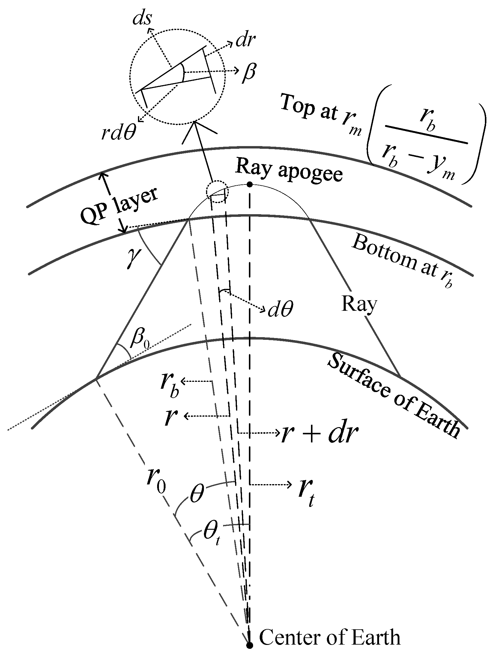
2.2. Ray Path Equations

Given the above quasi-parabolic model, ray path equations can be derived. Figure 1 illustrates the geometry of a ray trajectory in the quasi-parabolic layer, where the notations are defined as follows.

• $\beta$: ray elevation angle, i.e., the angle between ray path and the line that is parallel to the horizon;
• ${\beta }_0$: initial ray elevation angle, i.e., the value of $\beta$ when $r=r_0$;
• $r_t$: r at the top of the ray path;
• $\theta$: the angle between the line connecting the start point of the ray to the center of the earth and the line connecting the current position of the ray to the center of the earth;
• $\gamma$: the angle of the ray at the bottom of the ionosphere.

Figure 1. The geometry of the ray trajectory [32].

Figure 1. The geometry of the ray trajectory [32].

For ease of exposition, define the ratio of the OTHR operating frequency $f_w$ to the critical frequency of the layer $f_c$ as $f=f_w/f_c$. Accordingly, the refractive index of the layer at r is defined as [32]:

$${\mu }^2\left(r\right)=1-\frac{80.6N_e\left(r\right)}{f_w^2}=1-\frac{1}{f^2}+{\left(\frac{r_m-r}{f{y}_m}\right)}^2{\left(\frac{r_b}{r}\right)}^2$$

(2)

By Snell’s law [32], for the ray in Figure 1, the product $r\mu cos\beta$ is constant at any position in the layer, i.e., $r\mu cos\beta =r_{0}cos{\beta }_0$. Therefore, considering the geometry of the ray segments, the reflection by the ionosphere and the symmetry of the ray, the ground distance $R_D$ and the group path distance $R_P$ that the ray traverses are calculated as [32]:

$$\begin{array}{cc}\hfill & R_D=2r_0{\int }_0^{{\theta }_t}d\theta =2r_0{\int }_{r_0}^{r_t}\frac{dr}{rtan\beta }=2{\int }_{r_0}^{r_t}\frac{r_0^{2}cos{\beta }_0}{r\sqrt{r^2{\mu }^2-r_0^2{cos}^2{\beta }_0}}dr,\hfill \end{array}$$

(3)

$$\begin{array}{cc}\hfill & R_P=2{\int }_0^{S_t}\frac{ds}{\mu }=2{\int }_{r_0}^{r_t}\frac{dr}{\mu sin\beta }=2{\int }_{r_0}^{r_t}\frac{rdr}{\sqrt{r^2{\mu }^2-r_0^2{cos}^2{\beta }_0}},\hfill \end{array}$$

(4)

where $R_D$ is the distance measured along the earth’s surface, and $R_P$ is the distance that calculated as signal transit time multiplied by the light speed c, and $s_t$ is real ray path length at $r_t$. Given the definitions of all notations in the above equations, and based on standard integration table [39], the integrations in Equations (3) and (4) are calculated as:

$$\begin{array}{ll}{R}_D& \stackrel{\Delta }{=}\varphi (\mathit{\zeta },{\beta }_0)\\ & =2r_0\left[(\gamma -{\beta }_0)-\frac{r_{0}cos{\beta }_0}{2\sqrt{C}}\times ln\frac{B^2 - 4AC}{4C{\left(sin\gamma + \frac{1}{r_b}\sqrt{C} + \frac{1}{2\sqrt{C}}B\right)}^2}\right],\end{array}$$

(5)

$$\begin{array}{ll}{R}_P& \stackrel{\Delta }{=}\psi (\mathit{\zeta },{\beta }_0)\\ & =2\left(r_{b}sin\gamma -r_{0}sin{\beta }_0\right) + \frac{2}{A}\left[-r_{b}sin\gamma -\frac{B}{4\sqrt{A}}ln\frac{B^2 - 4AC}{{(2A{r}_b + B + 2r_b\sqrt{A}sin\gamma )}^2}\right],\end{array}$$

(6)

where $\gamma ={cos}^{-1}(r_0/r_{b}cos{\beta }_0)$ by the law of sines. The variables A, B and C are written as:

$$\begin{array}{cc}\hfill A& =1-\frac{1}{f^2}+{\left(\frac{r_b}{f{y}_m}\right)}^2,\hfill \end{array}$$

(7)

$$\begin{array}{cc}\hfill B& =-\frac{2r_m{r}_b^2}{f^2{y}_m^2},\hfill \end{array}$$

(8)

$$\begin{array}{cc}\hfill C& ={\left(\frac{r_b{r}_m}{f{y}_m}\right)}^2-r_0^2{cos}^2{\beta }_0.\hfill \end{array}$$

(9)

According to the above geometry, at the ray apogee, one has:

$$A{r}_t^2+B{r}_t+C=0.$$

The maximum of the ray height $r_{t,max}=-B/\left(2A\right)$. For ray tracing using other ionospheric electron density profile models, the reader is referred to [18,40,41].

2.3. Reference Sources and Targets Modeling

As we mentioned in Section 1, the reference sources may include HF beacons or transponders, terrain features, microwave radars, and airliners information from ADS-B and ships information from AIS.

Assume that there are L reference sources in the OTHR surveillance area. The ground range of reference source l $(l=1,\dots ,L)$ is denoted as ${\rho }^l$. The measurement of the ground range of the reference source l can be written as:

$$z^l={\rho }^l+u^l,$$

(10)

where $u^l$ is the Gaussian measurement noise with variance $U^l$. The variance is different for different type of reference sources. For example, the measurement noise of ADS-B is small comparing with the measurement noise of OTHR. Therefore, it can be ignored. So are the HF beacons and terrain features. The measurement set of all reference sources is written as: $\mathit{z}=\{z^1,\dots ,z^L\}$.

Denote the ground range of the targets of interest in the OTHR surveillance area by ${\overline{\rho }}^n$, where $n=1,\dots ,N$, and N is the number of targets. Note that the CR of each target is carried out separately. Some reference sources, such as airliners and ships could be targets of interest as well.

2.4. OTHR Measurement Modeling

Based on the above models, the OTHR measurement models of targets and reference sources are given here. We focus on the range accuracy of targets in CR; hence the related measurement is the group path distance in Equation (6). For each reference source or target, the measurement equation is written as,

$$y=\psi (\mathit{\zeta },{\beta }_0)+v,$$

(11)

where v is Gaussian white noise with variance V.

The measurement sets of all reference sources and interested targets are written as $\mathit{y}=\{y^1,\dots ,y^L\}$ and $\overline{\mathit{y}}=\{{\overline{y}}^1,\dots ,{\overline{y}}^N\}$, respectively. Meanwhile, the initial elevation angle sets of the rays that reach each reference source and interested target are written as ${\mathit{\beta }}_0=\{{\beta }_0^1,\cdots ,{\beta }_0^L\}$ and ${\overline{\mathit{\beta }}}_0=\{{\overline{\beta }}_0^1,\cdots ,{\overline{\beta }}_0^N\}$, respectively.

It is worth noting that, only few OTHR, such as French Nostradamus [21] can measure the elevation angle. Generally, the initial elevation angle ${\mathit{\beta }}_{\mathbf{0}}$ is unknown as we assume in this paper. Meanwhile, although the relationship between OTHR measurement y and reference source or target ground range $\rho$ in Equation (11) is not explicitly shown, the initial elevation angle ${\beta }_0$ determines whether the signal can be reflected back to the receiver via the reference source or the target, and OTHR measurement y is implicitly related to the reference source or the target ground range $\rho$ by ${\beta }_0$. In other words, the ground distance $R_D$ of the ray that reaches the reference source or the target is equal to the ground range of the reference source or the target, i.e.,

$$\rho =\varphi (\mathit{\zeta },{\beta }_0),$$

(12)

where $\varphi$ is defined as in Equation (5).

2.5. Problem Formulation

Our aim is to improve the accuracy of CR by inferring the ionospheric profile model parameters vector $\mathit{\zeta }$ from reference source data $\mathit{z}$ and their OTHR measurements $\mathit{y}$ and then performing the CR of the interested targets based on the inferred ionospheric parameters $\mathit{\zeta }$ and the measurements of the targets $\overline{\mathit{y}}$. Note that an important preliminary procedure to apply our method is to associate the reference sources with their corresponding OTHR measurements. This procedure is out of the scope of this paper. The reader is referred to [24,25,26]. In other words, we assume that the pair $(y^l,z^l)$ of a reference source and its corresponding OTHR measurement is known.

Based on the above-mentioned models, the block diagram of our problem, which consists of a typical inverse problem [42] and a forward model evaluation problem, is shown in Figure 2.

By Bayes’ rule, given the OTHR measurements $\mathit{y}$ and reference source data $\mathit{z}$, the joint posterior PDF of ionospheric parameters vector $\mathit{\zeta }$ and the initial elevation angle vector ${\mathit{\beta }}_0$ is written as:

$$p(\mathit{\zeta },{\mathit{\beta }}_{\mathbf{0}}\mid \mathit{y},\mathit{z})=\frac{p\left(\mathit{y}\mid \mathit{\zeta },{\mathit{\beta }}_{\mathbf{0}}\right)p\left(\mathit{z}\mid \mathit{\zeta },{\mathit{\beta }}_{\mathbf{0}}\right){\pi }_0(\mathit{\zeta },{\mathit{\beta }}_0)}{{\int }_{{\mathbb{R}}^{3+L}}p\left(\mathit{y}\mid \mathit{\zeta },{\mathit{\beta }}_{\mathbf{0}}\right)p\left(\mathit{z}\mid \mathit{\zeta },{\mathit{\beta }}_{\mathbf{0}}\right){\pi }_0(\mathit{\zeta },{\mathit{\beta }}_0)\mathrm{d}\mathit{\zeta }\mathrm{d}{\mathit{\beta }}_0},$$

(13)

where ${\pi }_0(\mathit{\zeta },{\mathit{\beta }}_0)$ is the joint prior distribution of $\mathit{\zeta }$ and ${\mathit{\beta }}_0$. The analytical solution of Equation (13) can not directly obtained because of the implicit OTHR measurement function. As will be shown in the next section, we resort to a sampling-based method.

Once the estimation of $\widehat{\mathit{\zeta }}$ is derived, the CR of the target of interest is performed, which includes two steps. The first step is to find the elevation angle ${\overline{\mathit{\beta }}}_0$ with OTHR measurement $\overline{\mathit{y}}$ and $\widehat{\mathit{\zeta }}$ through Equation (6) based on a dichotomy method. The second step is to calculate the ground distance with elevation angle ${\overline{\mathit{\beta }}}_0$ and $\widehat{\mathit{\zeta }}$ through Equation (5).

3. Solutions

In this section, the estimation of the ionospheric parameters and the CR process are introduced in detail. Firstly, the joint posterior PDF of ionospheric parameters $\mathit{\zeta }$ and the initial elevation angle ${\mathit{\beta }}_0$ is derived. Then, MCMC-based estimation of $\mathit{\zeta }$ is proposed, and the ESAI sampling method and its convergence evaluation are followed.

3.1. Derivation and Framework

Given $\mathit{\zeta }$ and ${\mathit{\beta }}_0$ of all rays that reach the reference sources, and assuming that the OTHR measurements $\mathit{y}$ are independent over different reference sources, the conditional PDF (measurement likelihood) of the OTHR measurements $\mathit{y}$ is written as:

$$\begin{array}{cc}\hfill p(\mathit{y}\mid \mathit{\zeta },{\mathit{\beta }}_0)& =\prod _{l=1}^{L}p\left(y^l-\psi (\mathit{\zeta },{\beta }_0^l)\right).\hfill \end{array}$$

(14)

Similarly, assuming reference sources data $\mathit{z}$ are independent, then the conditional PDF (measurement likelihood) of $\mathit{z}$ is written as:

$$p(\mathit{z}\mid \mathit{\zeta },{\mathit{\beta }}_0)=\prod _{l=1}^{L}p\left(z^l-\varphi (\mathit{\zeta },{\beta }_0^l)\right).$$

(15)

As the measurement noises $v^l$ in Equation (11) and $u^l$ in Equation (10) are both zero mean and Gaussian, the measurement likelihoods are written as:

$$\begin{array}{cc}\hfill y^l-\psi (\mathit{\zeta },{\beta }_0^l)& =v^l\sim \mathcal{N}(0,V^l),\hfill \end{array}$$

(16)

$$\begin{array}{cc}\hfill z^l-\psi (\mathit{\zeta },{\beta }_0^l)& =u^l\sim \mathcal{N}(0,U^l).\hfill \end{array}$$

(17)

Apparently, $\mathit{\zeta }$ and ${\mathit{\beta }}_0$ are independent, i.e., ${\pi }_0(\mathit{\zeta },{\mathit{\beta }}_0)={\pi }_0\left(\mathit{\zeta }\right){\pi }_0\left({\mathit{\beta }}_0\right),$ where ${\pi }_0\left(\mathit{\zeta }\right)$ is assumed to be Gaussian with mean ${\overline{\mathit{m}}}_0$ and covariance matrix ${\overline{\Sigma }}_0$. Initial elevation angles are independent as well. We assume that each initial elevation angle follows a continuous uniform distribution over a certain interval. That is, ${\pi }_0\left({\mathit{\beta }}_0\right)={\prod }_{l=1,\cdots ,L}{\pi }_0\left({\beta }_0^l\right)$, and ${\pi }_0\left({\beta }_0^l\right)=\mathcal{U}[{\lambda }_1,{\lambda }_2]$.

As the denominator in Equation (13) is a constant, Equation (13) is simplified as:

$$p(\mathit{\zeta },{\mathit{\beta }}_{\mathbf{0}}\mid \mathit{y},\mathit{z})\propto p\left(\mathit{y}\mid \mathit{\zeta },{\mathit{\beta }}_{\mathbf{0}}\right)p\left(\mathit{z}\mid \mathit{\zeta },{\mathit{\beta }}_{\mathbf{0}}\right){\pi }_0(\mathit{\zeta },{\mathit{\beta }}_0),$$

(18)

which is then expressed as:

$$\begin{array}{cc}\hfill lnp(\mathit{\zeta },{\mathit{\beta }}_{\mathbf{0}}\mid \mathit{y},\mathit{z})& \propto \sum _{l=1}^{L}lnp\left(y^l-\psi (\mathit{\zeta },{\beta }_0^l)\right)+\sum _{l=1}^{L}lnp\left(z^l-\varphi (\mathit{\zeta },{\beta }_0^l)\right)+ln{\pi }_0(\mathit{\zeta },{\mathit{\beta }}_0)\hfill \\ \hfill & =\sum _{l=1}^L\mathcal{D}\left(y^l-\psi (\mathit{\zeta },{\beta }_0^l),V^l\right)+\sum _{l=1}^L\mathcal{D}\left(z^l-\varphi (\mathit{\zeta },{\beta }_0^l),U^l\right)\hfill \\ \hfill & +\mathcal{D}\left(\mathit{\zeta }-{\overline{\mathit{m}}}_0,{\overline{\Sigma }}_0\right)+\left[\mathrm{items}\mathrm{independent}\mathrm{of}\mathit{\zeta }\mathrm{and}{\mathit{\beta }}_0\right],\hfill \end{array}$$

(19)

where the operator $\mathcal{D}(\mathit{x},\Sigma )$ denotes the operation $\mathcal{D}(\mathit{x},\Sigma )=-{\mathit{x}}^T{\Sigma }^{-1}\mathit{x}$.

Solving Equation (19) directly is intractable. This is because, firstly, from Equations (5), (6), (11) and (12), no explicit expression exists between the function $\psi (·)$ and the function $\varphi (·)$, (i.e., the reference source ground distance $\rho$ and the OTHR measurement y). Secondly, ${\mathit{\beta }}_0$ is a hidden variable. The fact that ${\mathit{\beta }}_0$ and $\mathit{\zeta }$ are coupled in the OTHR measurement process makes their relationship be expressed implicitly by equation ${\rho }^l=\varphi (\mathit{\zeta },{\beta }_0^l)$.

As the elevation angle vector ${\mathit{\beta }}_{\mathbf{0}}$ is also unknown in the ionospheric parameters estimation, there are $L+3$ variables to be estimated. If the measurement noise $u^l$ of reference sources (e.g., airliners with ADS-B, ships with AIS, HF beacons, and terrain features) in the ground coordinates is small, we let $z^l\approx {\rho }^l$ to reduce the computational cost. In this case, given $\mathit{\zeta }$, ${\beta }_0^l$ can be found based on $z^l$ through a dichotomy method.

$${\beta }_0^l={\varphi }^{-1}(\mathit{\zeta },z^l).$$

(20)

Accordingly, the dimension of the space of the estimated parameters is reduced from $L+3$ to 3. Equation (19) is then simplified as:

$$\begin{array}{cc}\hfill h\left(\mathit{\zeta }\right)\stackrel{\Delta }{=}lnp(\mathit{\zeta }\mid \mathit{y},\mathit{z})& \propto \sum _{l=1}^L\mathcal{D}\left[y^l-\psi \left(\mathit{\zeta },{\varphi }^{-1}(\mathit{\zeta },z^l)\right),V^l\right]+\mathcal{D}\left(\mathit{\zeta }-{\overline{\mathit{m}}}_0,{\overline{\Sigma }}_0\right)\hfill \\ \hfill & + \left[\mathrm{items}\mathrm{independent}\mathrm{of}\mathit{\zeta }\mathrm{and}{\mathit{\beta }}_0\right].\hfill \end{array}$$

(21)

If the measurement noise of the reference sources in the ground coordinates is too big to be ignored, which means the approximation $z^l\approx {\rho }^l$ cannot be applied, then simultaneous estimation of both the ionospheric parameters and the initial elevation angles is needed. We leave it as our future work.

Because of the complexity of the ray path equations mentioned above, a sampling-based method is adopted to solve Equation (21), which generates a set of samples to approximate the posterior PDF (21), and the estimation of $\mathit{\zeta }$ can be obtained. More specifically, Markov Chain Monte Carlo (MCMC) [43], which is a powerful algorithm framework for handling complicated inference problems, is used in this paper to estimate $\mathit{\zeta }$.

MCMC constructs a Markov chain (an ensemble of chains) that has (have) the desired distribution (e.g., the posterior PDF (21)) as its (their) equilibrium distribution. Then the samples of the desired distribution can be obtained by recording states from the chain. The simplest and most popular MCMC method is Metropolis-Hastings (MH) algorithm, of which the basic idea is as follows. Given the distribution $h\left(\mathit{\zeta }\right)$, a proposal distribution $q\left({\mathit{\zeta }}^{\prime }\right|\mathit{\zeta })$ and an initial value of $\mathit{\zeta }$, an MH step involves sampling a candidate value ${\mathit{\zeta }}^{\prime }$ according to $q\left({\mathit{\zeta }}^{\prime }\right|\mathit{\zeta })$ [44]. The Markov chain then moves towards ${\mathit{\zeta }}^{\prime }$ with the acceptance probability $a\left({\mathit{\zeta }}^{\prime }\right|\mathit{\zeta })=min\{1,{\left[h\left(\mathit{\zeta }\right)q\left({\mathit{\zeta }}^{\prime }\right|\mathit{\zeta })\right]}^{-1}h\left({\mathit{\zeta }}^{\prime }\right)q\left(\mathit{\zeta }\right|{\mathit{\zeta }}^{\prime })\}$; otherwise, it remains at $\mathit{\zeta }$. This process is repeated until enough samples are generated.

Denote the obtained samples by ${\left\{{\mathit{s}}_i\right\}}_{i=1}^{N_s}$. The minimum variance estimation of $\mathit{\zeta }$ is:

$$\widehat{\mathit{\zeta }}=\frac{1}{N_s}\sum _{i=1}^{N_s}{\mathit{s}}_i.$$

(22)

To use the samples of the Markov chain when it reaches its equilibrium distribution, which brings more accurate estimation, burn-in strategy is often used when exploiting MCMC-based method. That is, the samples generated at the beginning of an MCMC run, e.g., the first half, are throw away [45]. Additionally, the thinning technique [46,47] is used in order to reduce correlation between samples. That is, instead of keeping all samples, only every ${\xi }^{\mathrm{th}}$ (e.g., $\xi =10$) iteration is kept. At last, perform convergence test of the chain. If the chain converges, the generated samples are used to estimate the ionospheric parameters by Equation (22); otherwise, find alternative samplers. We summarize the complete procedure for the estimation of ionospheric parameters $\mathit{\zeta }$ as below.

(1)

Initialization. Using the prior distribution of the ionospheric parameters to initialize the sampler.

(2)

Sampling. Draw samples from the posterior PDF in Equation (21). The detailed sampling method will be descried in the following Section 3.2.

(3)

Burn-in. The beginning part, e.g., the first half, of the samples are throw away.

(4)

Thinning. Only every ${\xi }^{\mathrm{th}}$ (e.g., $\xi =10$) sample is kept.

(5)

Convergence evaluation. Determine if the Markov chain converges to the distribution (21) based on the method will be introduced in the following Section 3.3. If the Markov chain converges, go to next step; otherwise, find alternative samplers and go to Step 2.

(6)

Estimation. Using Equation (22) to estimate $\mathit{\zeta }$.

Note that no MCMC method exists which guarantees that the Markov chain converges to the desired distribution [48]. In Step 5 of the above procedure, if the number of samples exceeds the given maximum number of samples and the convergence of the Markov chain is not reached, one may need to adjust the parameters of the sampling method or resort to other sampling methods.

Note that the posterior PDF (21) is implicitly defined. We found that the standard MH method might need a long chain to sample from Equation (21), which is very time-consuming. Alternatively, an improved MCMC algorithm, namely ensemble samplers with affine invariance (ESAI) [49], is adopted to estimate ionospheric parameters and will be detailed in the next section.

3.2. ESAI Sampling

ESAI is particularly useful for sampling badly scaled distribution and can produce independent samples with a much shorter autocorrelation time than the standard MH method [49]. The details of ESAI sampling for the estimation of the ionospheric parameters are as follows. Let $\mathit{S}={\left\{{\mathit{s}}_i\left(t\right)\right\}}_{i=1,\dots ,I;t=1,\dots ,T_e}$ represent I chains which are also called stochastic processes of “walkers” that move around randomly in the space of $\mathit{\zeta }$, where $T_e$ is the length of each walker. For each walker i, its state is initialized as ${\mathit{s}}_i\left(1\right)={\overline{\mathit{m}}}_0$, which is the mean of the prior distribution of $\mathit{\zeta }$. For the choice of the number and the length of the walkers, the read is referred to [50].

Those walkers sample separately to generate samples from the distribution (21), which are denoted as the states of those walkers. The update of each walkers is according to the following rules [49].

The new state of i-th walker depends on the current states of the other $I-1$ walkers, i.e., the complementary set ${\mathit{S}}_{\left[i\right]}=\{{\mathit{s}}_j\left(t\right),\forall j\ne i\}$. To update the state of the i-th walker ${\mathit{s}}_i\left(t\right)$, a walker ${\mathit{s}}_j\left(t\right)$ is randomly and uniformly chosen from the complementary set ${\mathit{S}}_{\left[i\right]}$, and then the new candidate state of ${\mathit{s}}_i$ is computed as:

$${\mathit{s}}_i^{*}={\mathit{s}}_j\left(t\right)+d[{\mathit{s}}_i\left(t\right)-{\mathit{s}}_j\left(t\right)],$$

(23)

where d is a random variable sampled from the distribution $g\left(d\right)$. A feasible distribution of $g\left(d\right)$ is [49]:

$$g\left(d\right)\propto \left\{\begin{array}{cc}1/\sqrt{d}& \mathrm{if}d\in \left[1/\tau ,\tau \right],\hfill \\ 0& \mathrm{otherwise},\hfill \end{array}\right.$$

(24)

where the parameter $\tau$ is adjustable to improve performance.

If the new state of the walker $s_i^{*}$ is accepted with probability:

$$a=min\left(1,d^{M-1}\frac{h\left({\mathit{s}}_i^{*}\right)}{h\left({\mathit{s}}_i\left(t\right)\right)}\right),$$

(25)

where $M=3$ is the dimension of the parameter space and $h(·)$ is the distribution in Equation (21), set ${\mathit{s}}_i(t+1)={\mathit{s}}_i^{*}$; otherwise, set ${\mathit{s}}_i(t+1)={\mathit{s}}_i\left(t\right)$. The detailed single update step at t of all walkers is summarized in Algorithm 1. By repeating the update step in Algorithm 1, we can obtain the samples drawn from Equation (21).

Algorithm 1 A single update step of all walkers to sample from Equation (21)

1: for$i=1,\cdots ,I$do 2:    Randomly select a walker ${\mathit{s}}_j\left(t\right)$ with equal probability from the complementary set ${\mathit{S}}_{\left[i\right]}$; 3:    Sample d from the distribution $g\left(d\right)$ in Equation (24); 4:    Compute ${\mathit{s}}_i^{*}={\mathit{s}}_j\left(t\right)+d[{\mathit{s}}_i\left(t\right)-{\mathit{s}}_j\left(t\right)]$ by Equation (23); 5:    Compute ${\mathit{\beta }}_0^{*}=[{\beta }_0^{1,*},\dots ,{\beta }_0^{L,*}]$ by setting $\mathit{\zeta }={\mathit{s}}_i^{*}$ and Equation (20); 6:    Compute $a=d^{M-1}h(\mathit{\zeta }={\mathit{s}}_i^{*},{\mathit{\beta }}_0^{*})/h(\mathit{\zeta }={\mathit{s}}_i\left(t\right),{\mathit{\beta }}_{0,k}\left(t\right))$; 7:    Sample r from $\mathcal{U}\left[0,1\right]$; 8:    if $r\le a$ then 9:        ${\mathit{s}}_i(t+1)\leftarrow {\mathit{s}}_i^{*}$, ${\mathit{\beta }}_{0,k}(t+1)\leftarrow {\mathit{\beta }}_0^{*}$; 10:   else 11:      ${\mathit{s}}_i(t+1)\leftarrow {\mathit{s}}_i\left(t\right)$, ${\mathit{\beta }}_{0,k}(t+1)\leftarrow {\mathit{\beta }}_{0,k}\left(t\right)$; 12:    end if 13: end for

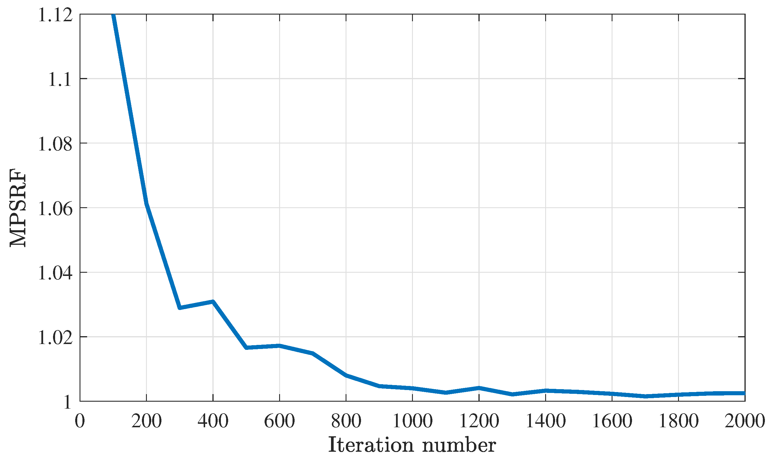
3.3. Convergence Evaluation

It is necessary to determine the convergence and the length of the Markov chain when using MCMC methods, for which various methods are available. For a recent review, the reader is referred to [51]. In this paper, the Gelman-Rubin (GR) diagnostic [52] and the graphical method [51] are used to heuristically evaluate the convergence of the sampler.

For ESAI, the GR diagnostic relies on multiple ensembles $\left\{{\mathit{S}}_1,{\mathit{S}}_2,\dots ,{\mathit{S}}_m\right\}$, each of which starts at different initial points and contains n samples. It is worth noting that, each ensemble ${\mathit{S}}_i$ is independently sampled using ESAI which includes I chains. One should not compute GR statistic using multiple chains in the same ensemble because the chains are not independent. Using those ensembles, GR calculates two estimators of the variance of $\mathit{S}$, namely within-ensemble variance estimate [52]:

$$W=\frac{1}{m(n-1)}\sum _{i=1}^m\sum _{j=1}^n\left({\mathit{S}}_{ij}-{\overline{\mathit{S}}}_i\right){\left({\mathit{S}}_{ij}-{\overline{\mathit{S}}}_i\right)}^T,$$

(26)

where ${\mathit{S}}_{ij}$ is the jth samples in ensemble ${\mathit{S}}_i$, and the pooled variance estimate [52]

$$\widehat{V}=\frac{n-1}{n}W+\frac{B}{n},$$

(27)

where

$$B=\frac{n}{m-1}\sum _{i=1}^m\left({\overline{\mathit{S}}}_i-\overline{\mathit{S}}\right){\left({\overline{\mathit{S}}}_i-\overline{\mathit{S}}\right)}^T$$

(28)

is the between-ensemble variance estimate, and ${\overline{\mathit{S}}}_i$ and $\overline{\mathit{S}}$ are the ith ensemble mean and the overall mean, respectively. Then the multivariate potential scale reduction factor (MPSRF) is used for convergence diagnostic, which is denoted by $\widehat{R}$ and given as [52]:

$$\widehat{R}=\frac{n-1}{n}+\left(1+\frac{1}{m}\right){\lambda }_1,$$

(29)

where ${\lambda }_1$ is the largest eigenvalue of the matrix $\left(W^{-1}B\right)/n$. Convergence is reached when $\widehat{R}$ sufficiently approaches to one.

The trace plot, which is a time series plot that shows the realization of the Markov chain at each iteration against the iteration numbers, is used to visualize how the Markov chain is moving around the parameter space. That is, how well the Markov chain is mixed which means how well it is close to its equilibrium distribution. The chain is likely to be converged only if the random-walk process crosses the domain of $\mathit{\zeta }$ many times during the MCMC run [48].

In addition, the autocorrelation time is also adopted to evaluate the convergence of the Markov chain. The lag-t autocorrelation is defined to be the correlation between the samples t steps apart. The autocorrelation plot shows the values of the lag-t autocorrelation function (ACF) $C_e\left(t\right)$ against increasing t values. For fast-mixing Markov chains, lag-t autocorrelation values drop down to zero quickly as t increases. The autocorrelation function $C_e\left(t\right)$ is defined as [50]:

$$C_e\left(t\right)=\underset{t^{\prime }\to \infty }{lim}cov\left[\mathit{S}\left(t^{\prime }+t\right),\mathit{S}\left(t^{\prime }\right)\right].$$

(30)

In practice, one can estimate $C_e\left(t\right)$ for a Markov chain of $N_s$ samples as:

$$C_e\left(t\right)\approx \frac{1}{N_s-t}\sum _{t^{\prime }=1}^{N_s-t}[\mathit{S}(t+t^{\prime })-\widehat{\mathit{\zeta }}][\mathit{S}\left(t^{\prime }\right)-\widehat{\mathit{\zeta }}],$$

(31)

where $\widehat{\mathit{\zeta }}$ is the mean of all samples and calculated in Equation (22).

4. Simulation and Analysis

In this section, numerical simulations are performed to verify the performance of proposed OTHR CR method based on MCMC. The method is implemented in Matlab R2018b and ran on an Inter (R) Core (TM) i5-4590 [email protected] computer.

4.1. Scenario Settings

The detailed parameter settings are given as follows. To show the performance of our proposed method, we generate 30-scan data, including the OTHR measurements and position of reference sources and interested targets. The sampling period $T^s=20$ s. It is assumed that the earth is a regular sphere, i.e., the radius of the earth $r_0=6371$ km is the same everywhere. The measurement noise standard deviation of the slant range $\sqrt{V^l}$ is 5 km. The true ionospheric parameters during the 30 scans are assumed to be time-varying and Gaussian with mean ${\mathit{m}}_0=[80\mathrm{km}+r_0,3.58\mathrm{MHz},20\mathrm{km}]$ and covariance ${\Sigma }_0=\mathrm{diag}\left({\mathit{\sigma }}^2\right)$, where $\mathit{\sigma }=[5\mathrm{km},0.2\mathrm{MHz},4\mathrm{km}]$. The prior distribution of the ionospheric parameters is also assumed to be Gaussian with the mean ${\overline{\mathit{m}}}_0=[79.2\mathrm{km}+r_0,3.6\mathrm{MHz},19.4\mathrm{km}]$ and the covariance ${\overline{\Sigma }}_0=\mathrm{diag}\left({\overline{\mathit{\sigma }}}^2\right)$, where $\overline{\mathit{\sigma }}=[4.96\mathrm{km},0.203\mathrm{MHz},4.11\mathrm{km}]$. We use ADS-B data of airliners and the corresponding OTHR measurements to illustrate the proposed CR scheme. Assume that there are 20 airliners and 20 interested targets moving in straight lines at constant speeds in the same azimuth direction within a relatively small subarea (400 km in range and 8° in azimuth) of OTHR coverage area.

The initial states of the airliners and the targets are found in

Table 1. Initial states of 20 airliners and 20 interested targets. The first two lines are the ground range ${\rho }^l$ (km) and ground range rate ${\dot{\rho }}^l$ (km/s) of each airliners. The last two lines are the ground range ${\rho }^l$ (km) and ground range rate ${\dot{\rho }}^l$ (km/s) of each interested targets.

1	2	3	4	5	6	7	8	9	10
1172.4	1344.1	1249.5	1155.8	1126.9	1177.2	1212.3	1288.3	1281.8	1229.8
−0.1084	−0.1183	0.1678	−0.1747	−0.0925	0.1551	0.1798	0.1775	−0.0920	0.1436
1177.1	1231.9	1096.0	1195.7	1006.2	1180.4	1310.3	1204.3	1234.8	1203.1
0.2032	0.1546	0.1692	−0.1716	0.1855	−0.1618	−0.1432	−0.1748	−0.1782	−0.1870
11	12	13	14	15	16	17	18	19	20
1070.4	1142.5	1363.2	1213.2	1086.4	1222.9	1089.2	1148.8	1150.5	1176.3
−0.1014	0.1851	−0.1232	−0.1054	0.1878	−0.1184	0.1924	−0.1541	0.1327	0.1544
1292.1	1218.7	1158.2	1318.5	1361.5	1343.8	1011.5	1188.4	1321.3	1368.1
−0.1906	0.1888	0.2132	0.1323	−0.0935	−0.1826	0.1702	−0.1446	−0.1587	−0.1473

. The measurements $\mathit{y}$ of 20 airliners received by OTHR at the first scan are shown in

Table 2. OTHR measurements of 20 targets at the first scan (slant range, km).

1	2	3	4	5	6	7	8	9	10
1192.4	1361.8	1274.1	1174.5	1147.3	1200.7	1238.3	1312.1	1299.5	1253.5
11	12	13	14	15	16	17	18	19	20
1089.5	1167.8	1378.8	1230.8	1112.1	1241.6	1114.4	1166.8	1172.3	1199.3

.

In order to visualize the posterior PDF of the ionospheric parameters in Equation (21), we show it in a selected cuboid parameter space with the boundary ${\mathit{m}}_0\pm [8\mathrm{km},0.6\mathrm{MHz},12\mathrm{km}]$. The selected parameter space is discretized into ${40}^3$ grids in the selected domain. The values of Equation (21) at these grid points calculated using the OTHR measurements of the first four airliners in Table 2 are shown in Figure 3. In Figure 3, the first three subgraphs are the planes where $y_m=20.9$ km, $f_c=3.69$ MHz, and $r_b-r_0=79.8$ km, respectively; the last subgraph is a corner of the selected parameter space in a 3D view.

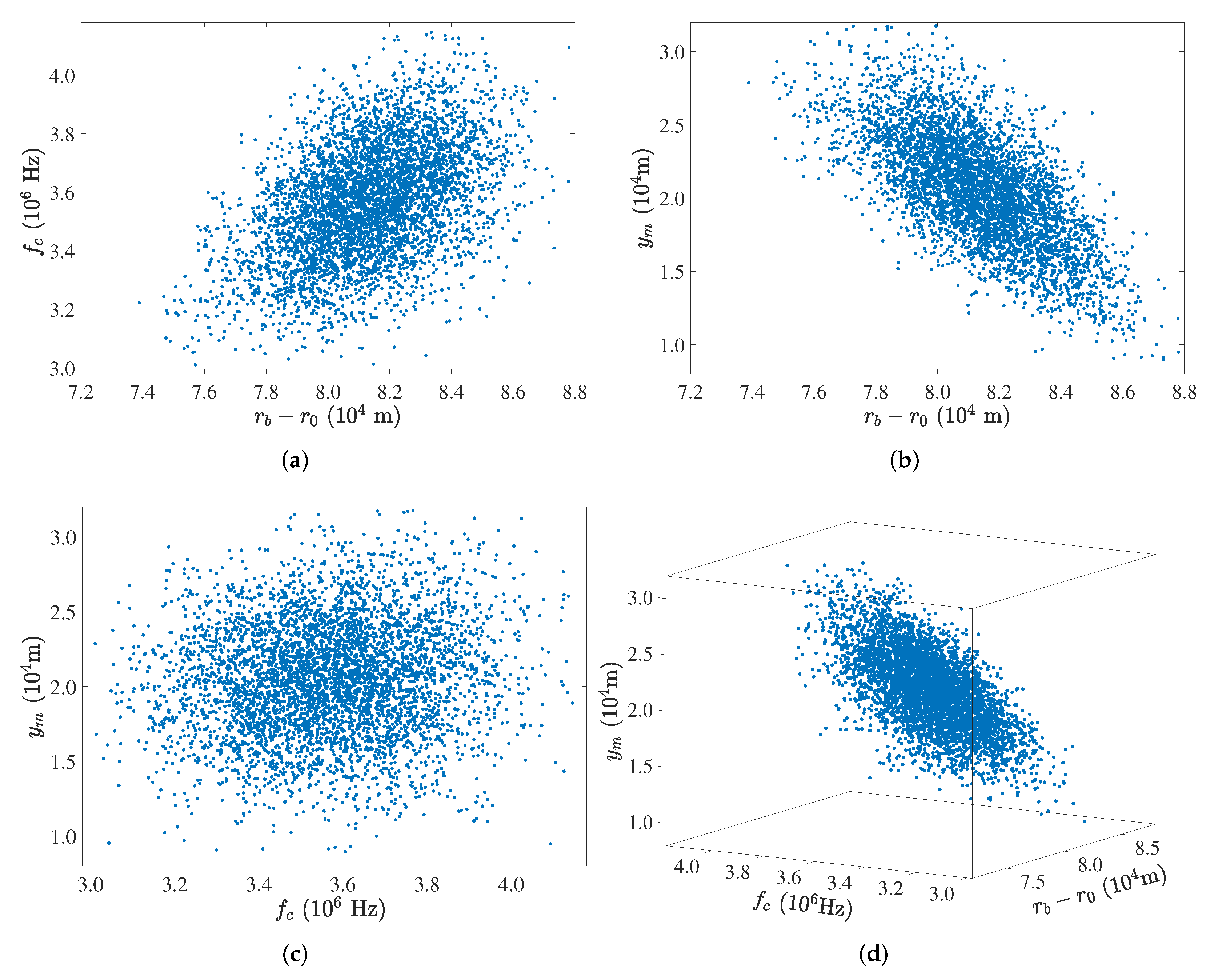
4.2. Convergence Evaluation of ESAI and Ionospheric Parameters Estimation

Before giving the convergence analysis of ESAI, an intuitive illustration of samples generated by ESAI is given. For ESAI, we use 100 walkers. 80,000 samples are sampled and only the latter half are taken due to the burn-in. At the same time, the thinning technique is used in order to reduce the correlation between samples. Finally, 4000 samples are obtained. The samples of the posterior PDF of the ionospheric parameters using the OTHR measurements of the first four airliners shown in Table 2 are shown in Figure 4. The samples are more dense in Figure 4 in the sub parameter space that the posterior PDF is large in Figure 3. Figure 3d and Figure 4d show the samples that correspond to the posterior PDF, which has intuitively verified the effectiveness of ESAI.

The GR diagnostic is performed in which four parallel ensembles are obtained for 2000 iterations starting at ${\overline{\mathit{m}}}_0\pm [0.2\mathrm{km},0.2\mathrm{MHz},0.1\mathrm{km}]$ and ${\overline{\mathit{m}}}_0\pm [0.4\mathrm{km},0.4\mathrm{MHz},0.2\mathrm{km}]$, respectively. The GR MPSRF is calculated base on these ensembles. The plots of iterative $\widehat{R}$ at the increment of every 100 iterations are given in Figure 5. It is seen that MPSRF approaches to one rapidly, which means that the used ESAI converges.

The convergence analysis of the samples in terms of the graphical method and the autocorrelation time is shown in Figure 6. Figure 6a shows the trace plots of the first 1000 samples and Figure 6b shows the autocorrelation plots of the Markov chain samples. From the track plots, it is seen that the chains are mixed well, i.e., the chains move around the parameter space many times and are not stuck in any region. At the same time, the autocorrelation of the samples is almost negligible after lag 15, which means the chains mix fast. In conclusion, the used ESAI sampler is effective and the parameter setting of the sampler is appropriate.

In order to evaluate the performance of the ESAI-based approach on ionospheric parameters estimation, different numbers of airliners are used. The ionospheric parameters estimation results are shown in Figure 7.

Table 3. Statistics on estimated ionospheric parameters in Figure 7. IR is the abbreviation of improvement ratio.

Statistic	${\mathit{r}}_{\mathit{b}}$		${\mathit{f}}_{\mathit{c}}$		${\mathit{y}}_{\mathit{m}}$
	Mean (km)	IR	Mean (kHz)	IR	Mean (km)	IR
4 airliners	2.11	58.33%	190.99	4.98%	3.76	7.09%
8 airliners	1.93	61.98%	189.02	5.96%	3.71	8.17%
12 airliners	1.80	64.41%	184.56	8.18%	3.65	9.75%
16 airliners	1.75	65.46%	184.01	8.45%	3.63	10.30%
20 airliners	1.73	65.89%	183.30	8.80%	3.61	10.74%

shows the mean values of the ionospheric parameter estimation in each dimension in 30 scans under different airliner numbers in Figure 7, and the improvement ratio compared with the a prior values. By observing Figure 7 and Table 3, it is seen that, the RMSEs of the ionospheric parameters $r_b$, $f_c$ and $y_m$ are reduced to 1.73 km, 183.3 kHz and 3.61 km, respectively, when using the ADS-B data of 20 airlines, and the corresponding improvement ratio compared with the a prior values are 65.89%, 8.8%, and 10.74%, respectively. Meanwhile, as we expected, as the number of airliners increases, the estimation error of the ionospheric parameters decreases. Overall, the accuracy of the ionospheric parameters are effectively improved when utilizing the proposed method with reference sources.

4.3. Analysis of OTHR CR Results

Given the effectiveness of ESAI in the last section, this section conducts statistical analysis of the results of the OTHR CR scheme proposed in Section 3. With OTHR measurements, the following three cases are considered for comparison.

• Case 1: The ground ranges of targets are calculated using the a prior of the ionospheric parameters;
• Case 2: The ground ranges of targets are calculated using the true ionospheric parameters;
• Case 3: The ground ranges of targets are calculated using the estimation of ionospheric parameters with ADS-B data of different number of airliners (i.e., 4, 8, 12, 16, 20 airliners).

The results of the three cases are compared with the true ground ranges of targets to analyze the improvement of the proposed OTHR CR method.

Figure 8 shows the RMSE comparison of the target ground ranges during OTHR CR under the three cases.

Table 4. Statistics of target ground range errors estimated under different cases in Figure 8 (the last five columns are the statistics of Case 3 with the estimation of ionospheric parameters with ADS-B data of 4, 8, 12, 16, 20 airliners.)

Cases	1	2	3(4)	3(8)	3(12)	3(16)	3(20)
RMSE mean(km)	2.86	1.01	1.13	1.08	1.06	1.05	1.04
Improvement ratio	-	-	60.39%	62.26%	63.07%	63.43%	63.66%

shows the RMSE mean values(m) of each curves over 30 scans in Figure 8, and the improvement ratios of Case 3 with respect to Case 1. From Figure 8 and Table 4, it is seen that, comparing with using the a prior ionospheric parameters, the RMSE of ground range is reduced from 2.86 to 1.04 km when using ionospheric parameters which are estimated with ADS-B data of 20 airliners and the corresponding improvement ratio is 63.66%. Overall, the more accurate the ionospheric parameters, the smaller the RMSE of the ground range during OTHR CR. The results show that the error of OTHR CR is reduced when using reference sources. The effectiveness of the proposed OTHR CR method is verified.

We emphasize that this improvement ratio may be relevant to the model of ionospheric electron density profile and is related to how close are the reference sources to the interested targets. In this paper, we use the quasi-parabolic model. As we mentioned in Section 2.1, the method can be applied to other models. Any model is a simplified and an approximate representation of the real and complicated ionosphere using mathematical expressions with parameters. The difference when applying different models of ionospheric electron density profile to our problem is that the to-be-estimated parameters are different. In general, the more complex the model is, the more accurate the representation, the more parameters we need to estimate, and the more computationally expensive the estimation of the parameters. We leave the evaluation of our proposed method when exploiting different models of ionospheric electron density profile as our future work. In our simulation, we have assumed that the reference sources and the interested targets are distributed in a relatively small area such that their corresponding signals are reflected via a neighbouring small ionospheric area. Intuitively, the closer the reference sources to the interested targets, the more accurate of the parameter estimation is. In practice, reference sources may be distributed in a large area or even in the entire OTHR coverage area. In this case, all the information of the reference sources and the corresponding OTHR measurements are collectively used to estimate the parameters together with the model of the ionospheric electron density profile, which potentially provides improvement on the estimation of all the parameters globally.

5. Conclusions

We proposed a novel method for OTHR CR through using MCMC to estimate the ionospheric parameters with reference sources. The quasi-parabolic model was used to describe ionospheric electron density profile. The estimation of the ionospheric parameters was formulated as a Bayesian inverse problem, which was then solved by an MCMC method, namely ESAI, due to the complicated ray path equation. The entire implementation procedure of ESAI for the estimation problem was described, followed by a description of convergence evaluation of ESAI using two different methods. Then the OTHR CR was performed based on the estimated ionospheric parameters. The simulation results have shown that, the estimated ionospheric parameters are more accurate comparing with the a prior value of ionospheric parameters, which in turn greatly reduced the OTHR CR error of interested targets. For future work, we plan to apply the proposed method to more models of ionospheric electron density profile and evaluate the corresponding improvement on OTHR CR. We will also consider using the OTHR measurements of reference sources via mixed-mode propagation to further reduce CR error.

References

1. Fabrizio, G.A. High Frequency Over-the-Horizon Radar: Fundamental Principles, Signal Processing, and Practical Applications; McGraw Hill Education: New York, NY, USA, 2013. [Google Scholar]
2. Ferraro, E.J.; Bucknam, J.N. Improved over-the-horizon radar accuracy for the counter drug mission using coordinate registration enhancements. In Proceedings of the 1997 IEEE National Radar Conference, Syracuse, NY, USA, 13–15 May 1997; pp. 132–137. [Google Scholar] [CrossRef]
3. Pulford, G.W.; Evans, R.J. A multipath data association tracker for over-the-horizon radar. IEEE Trans. Aerosp. Electron. Syst. 1998, 34, 1165–1183. [Google Scholar] [CrossRef]
4. Earl, G.F.; Ward, B.D. The frequency management system of the Jindalee over-the-horizon backscatter HF radar. Radio Sci. 1987, 22, 275–291. [Google Scholar] [CrossRef]
5. Pulford, G.; Logothetis, A.; Evans, R. Integrated Multipath Track Initiation for Over-the-Horizon Radar: 3rd Report to Telecom Australia; Technical report; University of Melbourne: Parkville, Australia, 1995. [Google Scholar]
6. Lan, H.; Ma, J.; Wang, Z.; Pan, Q.; Xu, X. A message passing approach for multiple maneuvering target tracking. Signal Process. 2020, 174, 107621. [Google Scholar] [CrossRef]
7. Guo, Z.; Wang, Z.; Lan, H.; Pan, Q.; Lu, K. OTHR multitarget tracking with a GMRF model of ionospheric parameters. Signal Process. 2021, 182, 107940. [Google Scholar] [CrossRef]
8. Percival, D.J.; White, K.A.B. Multihypothesis fusion of multipath over-the-horizon radar tracks. Signal Data Process. Small Targets 1998, 3373, 440–451. [Google Scholar] [CrossRef]
9. Kong, M.; Wang, G.; Wang, Y. Coordinate registration algorithms for over-the-horizon radar. J. Syst. Eng. Electron. 2006, 17, 725–730. [Google Scholar] [CrossRef]
10. Lan, H.; Liang, Y.; Wang, Z.; Yang, F.; Pan, Q. Distributed ECM Algorithm for OTHR Multipath Target Tracking with Unknown Ionospheric Heights. IEEE J. Sel. Top. Signal Process. 2018, 12, 61–75. [Google Scholar] [CrossRef]
11. Sathyan, T.; Chin, T.J.; Arulampalam, S.; Suter, D. A multiple hypothesis tracker for multitarget tracking with multiple simultaneous measurements. IEEE J. Sel. Top. Signal Process. 2013, 7, 448–460. [Google Scholar] [CrossRef]
12. Lan, H.; Liang, Y.; Pan, Q.; Yang, F.; Guan, C. An EM algorithm for multipath state estimation in OTHR target tracking. IEEE Trans. Signal Process. 2014, 62, 2814–2826. [Google Scholar] [CrossRef]
13. Lan, H.; Sun, S.; Wang, Z.; Pan, Q.; Zhang, Z. Joint target detection and tracking in multipath environment: A variational Bayesian approach. IEEE Trans. Aerosp. Electron. Syst. 2020, 56, 2136–2156. [Google Scholar] [CrossRef] [Green Version]
14. Wang, J.; Yang, B.; Wang, W.; Bi, Y. Multiple-detection multi-target tracking with labelled random finite sets and efficient implementations. IET Radar Sonar Navig. 2019, 13, 272–282. [Google Scholar] [CrossRef]
15. Feng, X.; Liang, Y.; Zhou, L.; Jiao, L.; Wang, Z. Joint mode identification and localisation improvement of over-the-horizon radar with forward-based receivers. IET Radar Sonar Navig. 2014, 8, 490–500. [Google Scholar] [CrossRef]
16. Pulford, G.W. OTHR multipath tracking with uncertain coordinate registration. IEEE Trans. Aerosp. Electron. Syst. 2004, 40, 38–56. [Google Scholar] [CrossRef]
17. Geng, H.; Liang, Y.; Cheng, Y. Target state and Markovian jump ionospheric height bias estimation for OTHR tracking systems. IEEE Trans. Syst. Man, Cybern. Syst. 2018, 50, 2599–2611. [Google Scholar] [CrossRef]
18. Jones, R.M.; Stephenson, J.J. A Versatile Three-Dimensional Ray Tracing Computer Program for Radio Waves in the Ionosphere; US Department of Commerce, Office of Telecommunications: Boulder, FL, USA, 1975; Volume 1.
19. Anderson, R.H.; Krolik, J.L. Track association for over-the-horizon radar with a statistical ionospheric model. IEEE Trans. Signal Process. 2002, 50, 2632–2643. [Google Scholar] [CrossRef]
20. Bourgeois, D.; Morisseau, C.; Flecheux, M. Quasi-parabolic ionosphere modeling to track with Over-the-horizon Radar. In Proceedings of the IEEE/SP 13th Workshop on Statistical Signal Processing, Bordeaux, France, 17–20 July 2005; pp. 962–965. [Google Scholar] [CrossRef]
21. Bourgeois, D.; Morisseau, C.; Flecheux, M. Over-the-horizon radar target tracking using multi-quasi-parabolic ionospheric modelling. IEE Proc.-Radar Sonar Navig. 2006, 153, 409–416. [Google Scholar] [CrossRef]
22. Romeo, K.; Bar-Shalom, Y.; Willett, P. Detecting low SNR tracks with OTHR using a refraction model. IEEE Trans. Aerosp. Electron. Syst. 2017, 53, 3070–3078. [Google Scholar] [CrossRef]
23. Wheadon, N.S.; Whitehouse, J.C.; Milsom, J.D.; Herring, R.N. Ionospheric modelling and target coordinate registration for HF sky-wave radars. In Proceedings of the 1994 Sixth International Conference on HF Radio Systems and Techniques, York, UK, 4–7 July 1994; pp. 258–266. [Google Scholar] [CrossRef]
24. Weijers, B.; Choi, D.S. OTH-B coordinate registration experiment using an HF beacon. In Proceedings of the Proceedings International Radar Conference, Alexandria, VA, USA, 8–11 May 1995; pp. 49–52. [Google Scholar] [CrossRef] [Green Version]
25. Barnum, J.R.; Simpson, E.E. Over-the-horizon radar target registration improvement by terrain feature localization. Radio Sci. 1998, 33, 1077–1093. [Google Scholar] [CrossRef]
26. Cuccoli, F.; Facheris, L.; Sermi, F. Coordinate registration method based on sea/land transitions identification for over-the-horizon sky-wave radar: Numerical model and basic performance requirements. IEEE Trans. Aerosp. Electron. Syst. 2011, 47, 2974–2985. [Google Scholar] [CrossRef]
27. Fabrizio, G.; Zadoyanchuk, A.; Francis, D.; Nguyen, V. Using emitters of opportunity to enhance track geo-registration in HF over-the-horizon radar. In Proceedings of the 2016 IEEE Radar Conference (RadarConf), Philadelphia, PA, USA, 2–6 May 2016; pp. 1–5. [Google Scholar] [CrossRef]
28. Holdsworth, D.A. Skywave over-the-horizon radar track registration using earth surface and infrastructure backscatter. In Proceedings of the 2017 IEEE Radar Conference (RadarConf), Seattle, WA, USA, 8–12 May 2017; pp. 986–991. [Google Scholar] [CrossRef]
29. Li, C.; Wang, Z.; Zhang, Z.; Lan, H.; Lu, K. Sea/Land clutter recognition for Over-the-horizon radar via deep CNN. In Proceedings of the 2019 International Conference on Control, Automation and Information Sciences (ICCAIS), Chengdu, China, 23–26 October 2019; pp. 1–5. [Google Scholar] [CrossRef]
30. Torrez, W.C.; Yssel, W.J. Associating microwave radar tracks with relocatable over-the-horizon radar (ROTHR) tracks using the advanced tactical workstation. In Proceedings of the Conference Record of Thirty-Second Asilomar Conference on Signals, Systems and Computers (Cat. No. 98CH36284), Pacific Grove, CA, USA, 1–4 November 1998; Volume 1, pp. 618–622. [Google Scholar] [CrossRef]
31. Bilitza, D. Ionospheric models for radio propagation studies. In The Review of Radio Science 1999–2002; Stone, W.R., Ed.; IEEE Press: Piscataway, NJ, USA, 2002; pp. 625–680. [Google Scholar]
32. Croft, T.A.; Hoogasian, H. Exact ray calculations in a quasi-parabolic ionosphere with no magnetic field. Radio Sci. 1968, 3, 69–74. [Google Scholar] [CrossRef]
33. Feng, J.; Ni, B.; Lou, P.; Wei, N.; Yang, L.; Liu, W.; Zhao, Z.; Li, X. A new inversion algorithm for HF sky-wave backscatter ionograms. Adv. Sp. Res. 2018, 61, 2593–2608. [Google Scholar] [CrossRef]
34. Yang, L.; Gao, H.; Ling, Y.; Li, B. Localization method of wide-area distribution multistatic sky-wave Over-the-Horizon radar. IEEE Geosci. Remote Sens. Lett. 2020, in press. [Google Scholar] [CrossRef]
35. Ding, M.; Tong, P.; Wei, Y.; Yu, L. Multiple phase screen modeling of HF wave field scintillations caused by the irregularities in inhomogeneous media. Radio Sci. 2021, 56, e2020RS007239. [Google Scholar] [CrossRef]
36. Langmuir, I. Oscillations in Ionized Gases. Proc. Natl. Acad. Sci. USA 1928, 14, 627–637. [Google Scholar] [CrossRef] [Green Version]
37. Galkin, I.; Reinisch, B.; Huang, X.; Bilitza, D. Assimilation of GIRO data into a real-time IRI. Radio Sci. 2012, 47, 1–10. [Google Scholar] [CrossRef]
38. Ippolito, A.; Altadill, D.; Scotto, C.; Blanch, E. Oblique ionograms automatic scaling algorithm OIASA application to the ionograms recorded by Ebro observatory ionosonde. J. Sp. Weather Sp. Clim. 2018, 8, 1–11. [Google Scholar] [CrossRef] [Green Version]
39. Lide, D.R. CRC Handbook of Chemistry and Physics, 97th ed.; CRC Press: New York, NY, USA, 2016. [Google Scholar] [CrossRef]
40. Coleman, C.J. Point-to-point ionospheric ray tracing by a direct variational method. Radio Sci. 2011, 46. [Google Scholar] [CrossRef]
41. Azzarone, A.; Bianchi, C.; Pezzopane, M.; Pietrella, M.; Scotto, C.; Settimi, A. IONORT: A Windows software tool to calculate the HF ray tracing in the ionosphere. Comput. Geosci. 2012, 42, 57–63. [Google Scholar] [CrossRef] [Green Version]
42. Stuart, A.M. Inverse problems: A Bayesian perspective. Acta Numer. 2010, 19, 451–559. [Google Scholar] [CrossRef] [Green Version]
43. Bishop, C.M. Pattern Recognition and Machine Learning; Springer: New York, NY, USA, 2006. [Google Scholar] [CrossRef]
44. Andrieu, C.; De Freitas, N.; Doucet, A.; Jordan, M.I. An introduction to MCMC for machine learning. Mach. Learn. 2003, 50, 5–43. [Google Scholar] [CrossRef] [Green Version]
45. Brooks, S.; Gelman, A.; Jones, G.; Meng, X.L. Handbook of Markov chain Monte Carlo; CRC Press: Boca Raton, FL, USA, 2011. [Google Scholar] [CrossRef]
46. Raftery, A.E.; Lewis, S.M. Implementing MCMC. In Markov Chain Monte Carlo Pract; Gilks, W.R., Richardson, S., Spiegelhalter, D., Eds.; Chapman & Hall/CRC Interdisciplinary Statistics, Taylor & Francis: London, UK, 1995. [Google Scholar] [CrossRef]
47. Link, W.A.; Eaton, M.J. On thinning of chains in MCMC. Methods Ecol. Evol. 2012, 3, 112–115. [Google Scholar] [CrossRef]
48. Hogg, D.W.; Foreman-Mackey, D. Data analysis recipes: Using Markov chain Monte Carlo. Astrophys. J. Suppl. Ser. 2018, 236, 11. [Google Scholar] [CrossRef] [Green Version]
49. Goodman, J.; Weare, J. Ensemble samplers with affine invariance. Commun. Appl. Math. Comput. Sci. 2010, 5, 65–80. [Google Scholar] [CrossRef]
50. Foreman-Mackey, D.; Hogg, D.W.; Lang, D.; Goodman, J. emcee: The MCMC hammer. Publ. Astron. Soc. Pacific 2013, 125, 306–312. [Google Scholar] [CrossRef] [Green Version]
51. Roy, V. Convergence diagnostics for Markov chain Monte Carlo. Annu. Rev. Stat. Appl. 2020, 7, 387–412. [Google Scholar] [CrossRef] [Green Version]
52. Brooks, S.P.; Gelman, A. General methods for monitoring convergence of iterative simulations. J. Comput. Graph. Stat. 1998, 7, 434–455. [Google Scholar] [CrossRef] [Green Version]
Figure 2. Block diagram of CR (Coordinate registration) based on reference sources.
Electronics 10 03086 g002
Figure 3. Grid-calculated and normalized PDF (probability distribution function) with four airliners OTHR (over-the-horizon radar) measurements. Views of different cut planes and 3D perspective.
Electronics 10 03086 g003
Figure 4. Plot of samples in different planes of projection and 3D views.
Electronics 10 03086 g004
Figure 5. Iterative MPSRF (multivariate potential scale reduction factor) plot for the independent ensembles.
Electronics 10 03086 g005
Figure 6. Normalized autocorrelation function and the integrated autocorrelation time of the samples.
Electronics 10 03086 g006
Figure 7. Statistical results of ionospheric parameter estimates for different target numbers.
Electronics 10 03086 g007
Figure 8. Statistical results of target ground range accuracy under different cases. In (b), the curves are obtained by using estimated ionospheric parameters with ADS-B data of different number of airliners (i.e., 4, 8, 12, 16, 20 airliners).
Electronics 10 03086 g008