
Design of a Lightweight Multilayered Composite for DC to 20 GHz Electromagnetic Shielding


 , ,
, ,
Abstract
:1. Introduction
2. Materials and Electromagnetic Model
2.1. Materials
2.2. Analytical Models
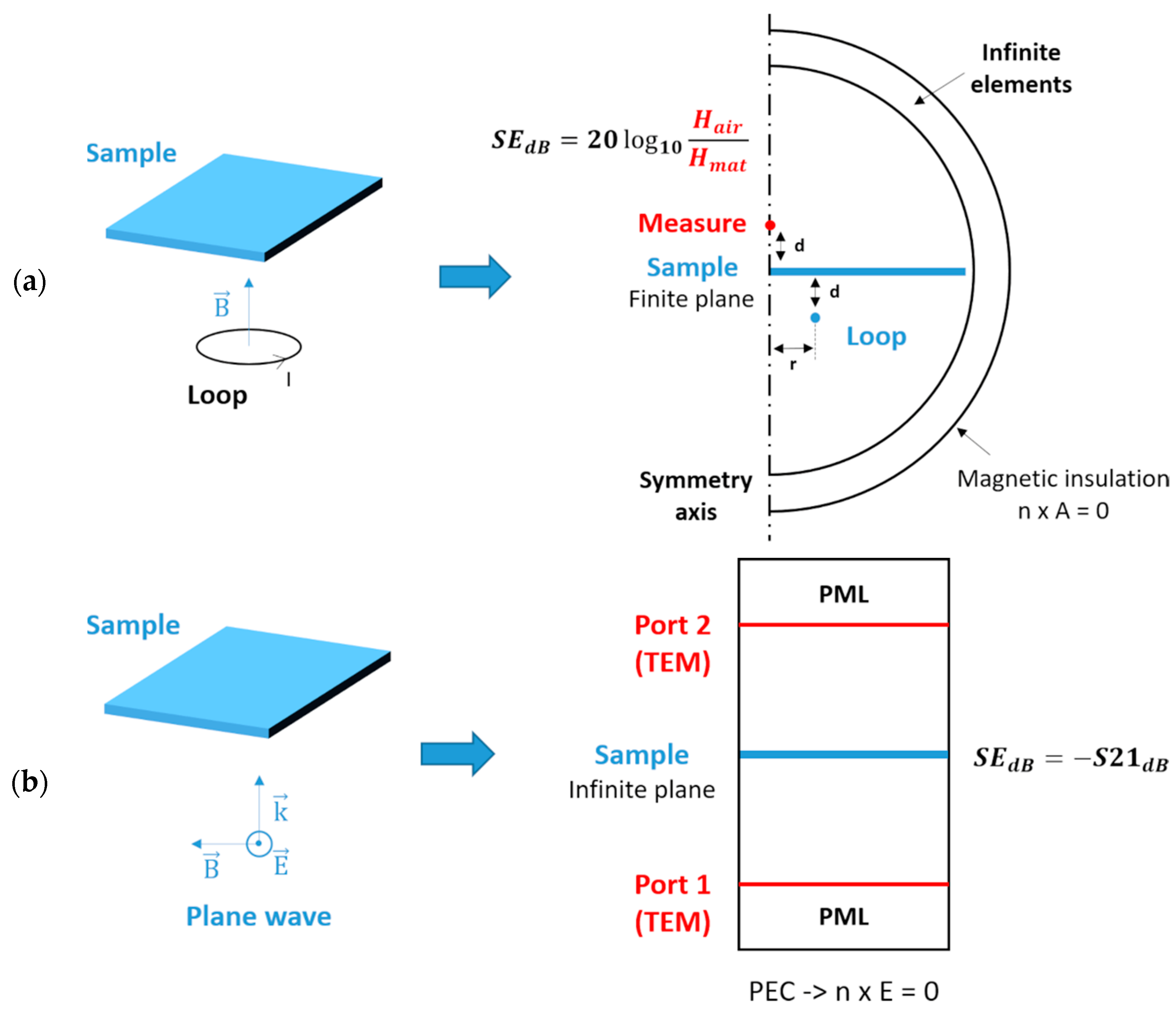
2.3. Numerical Models
3. Results and Discussion
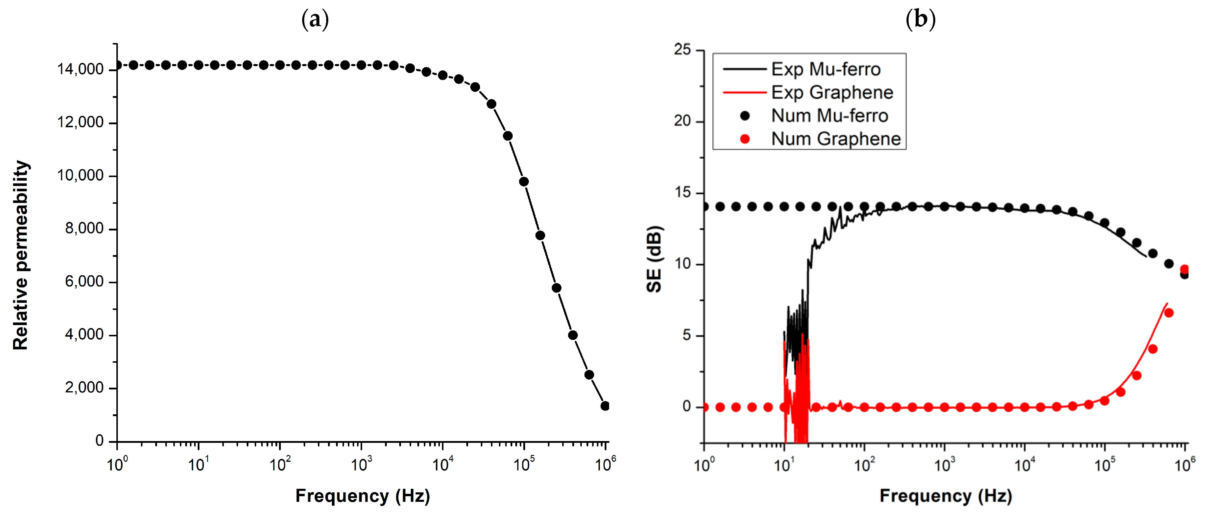
3.1. Relative Permeability of the Mu-Ferro and SE of One-Material Sheet
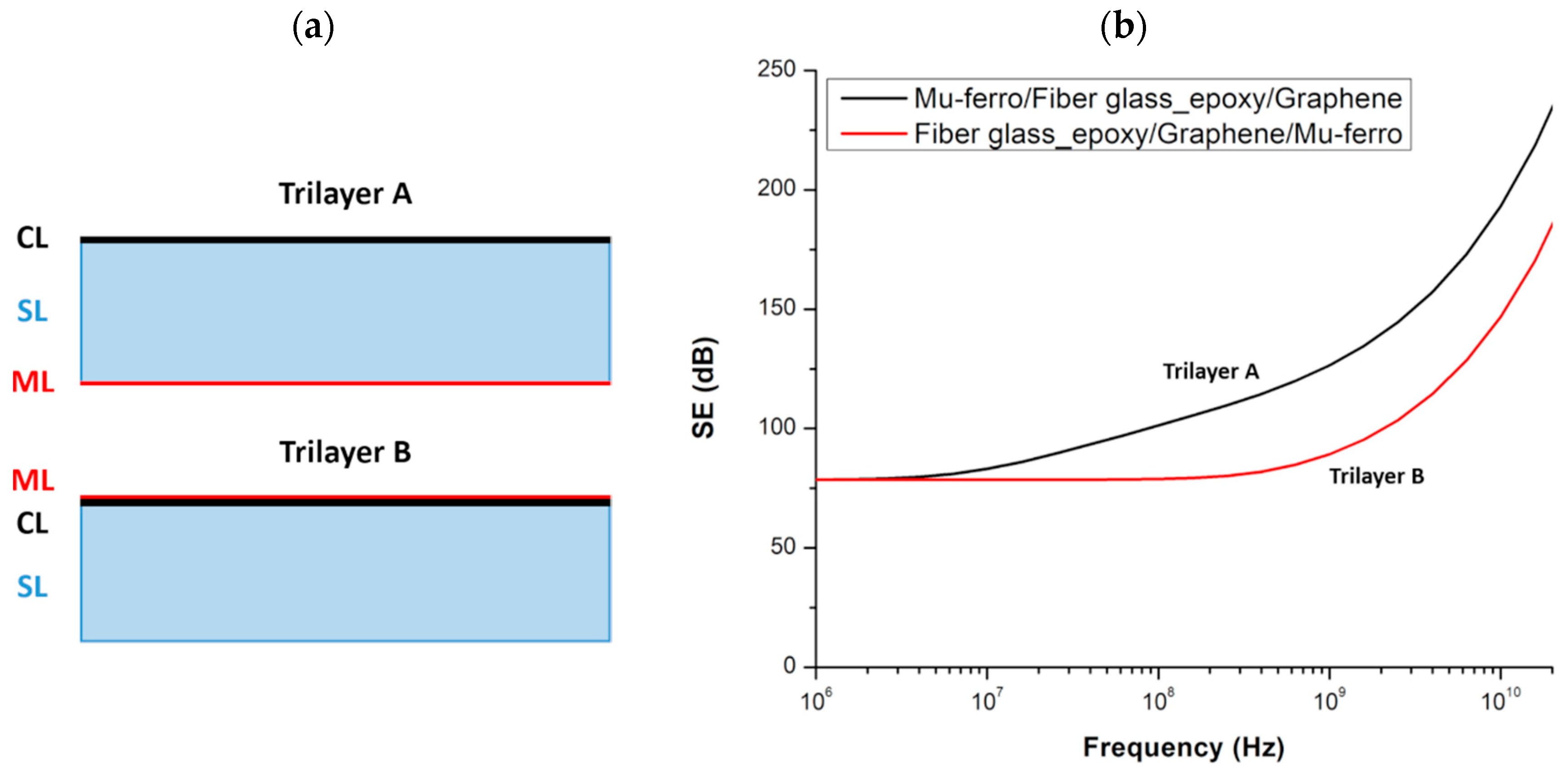
3.2. Layer Arrangements
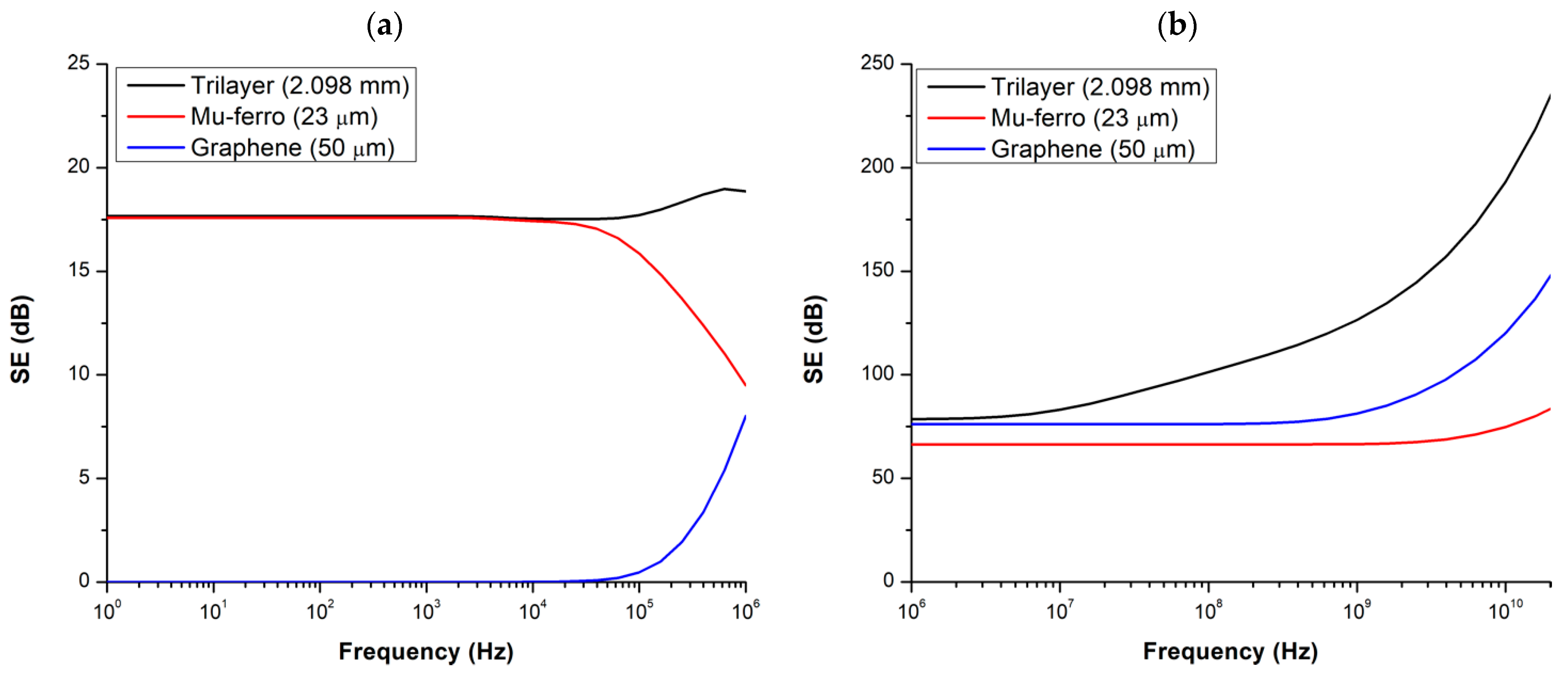
3.3. Materials Contribution
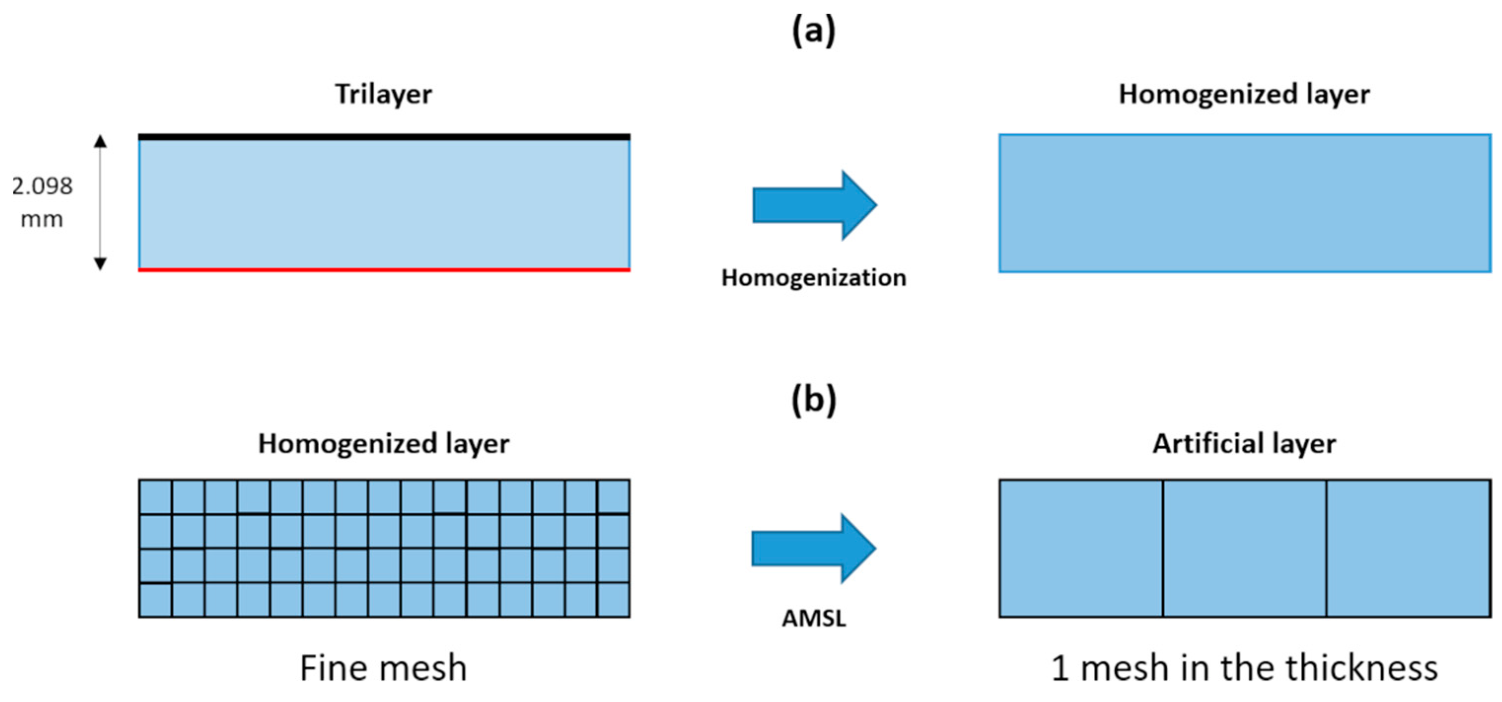
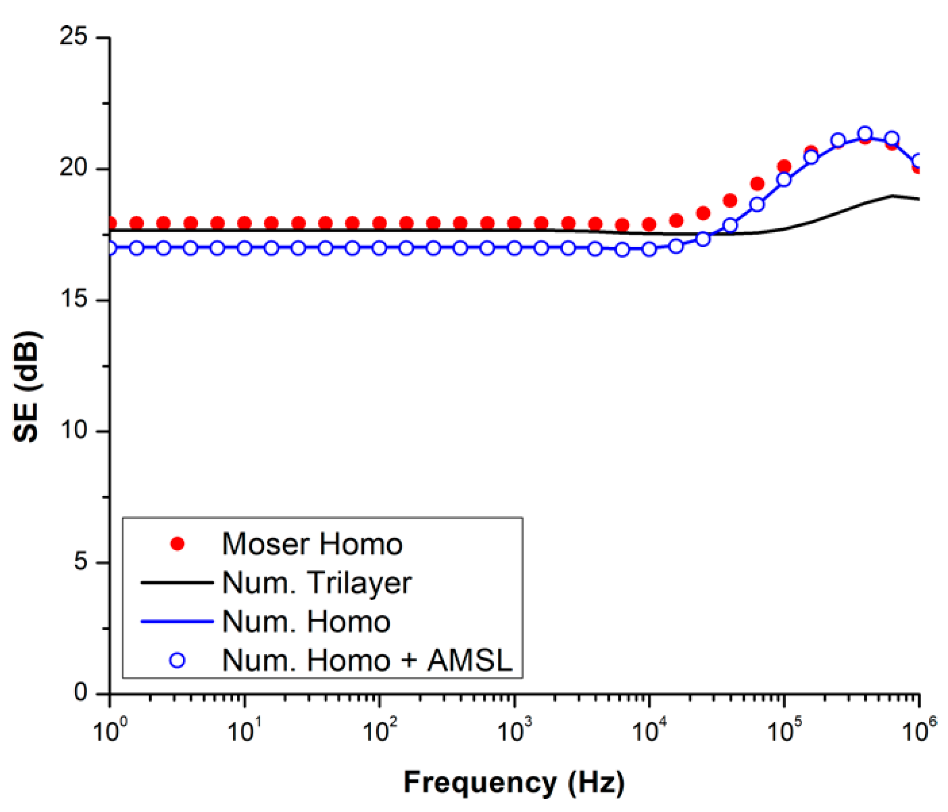
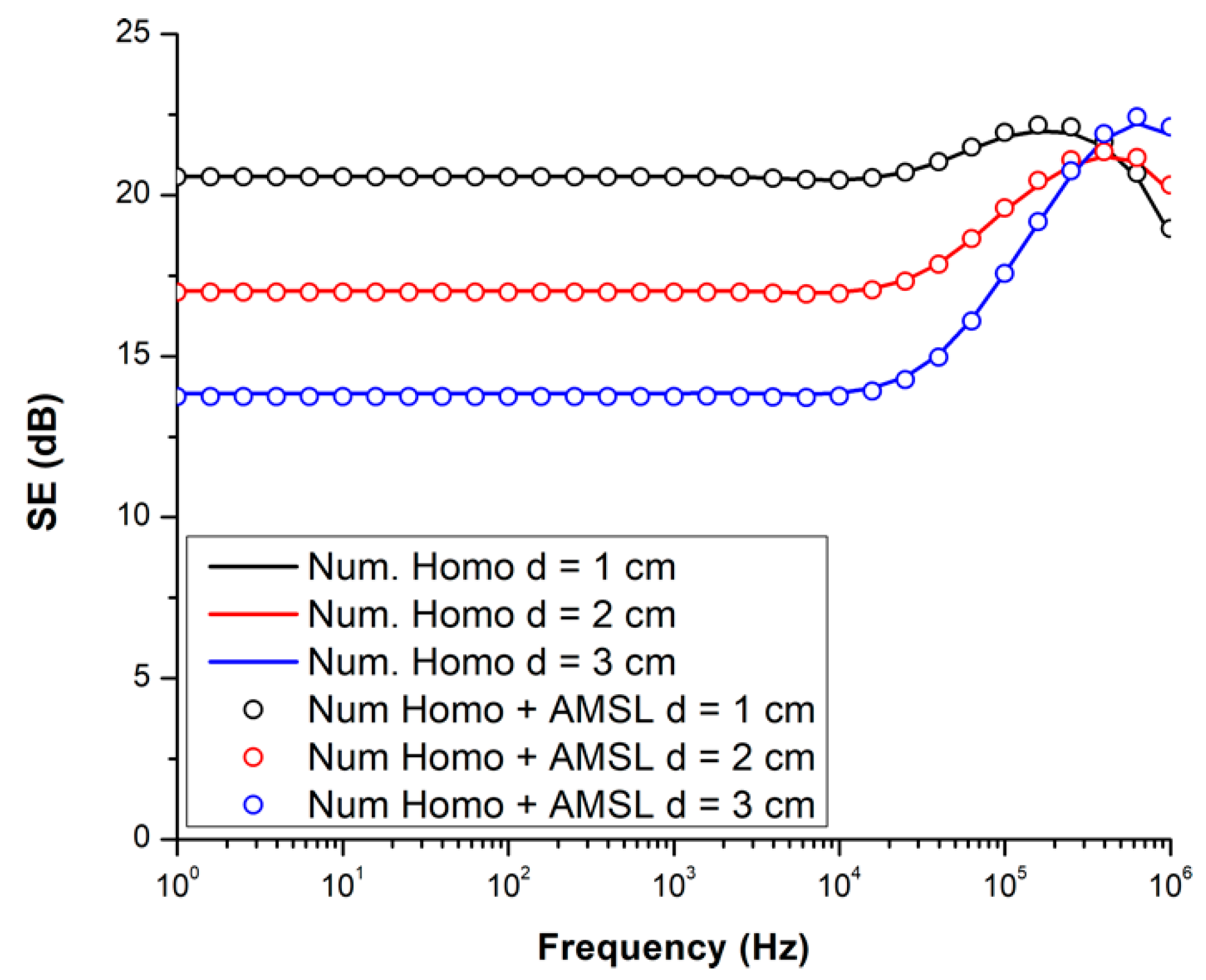
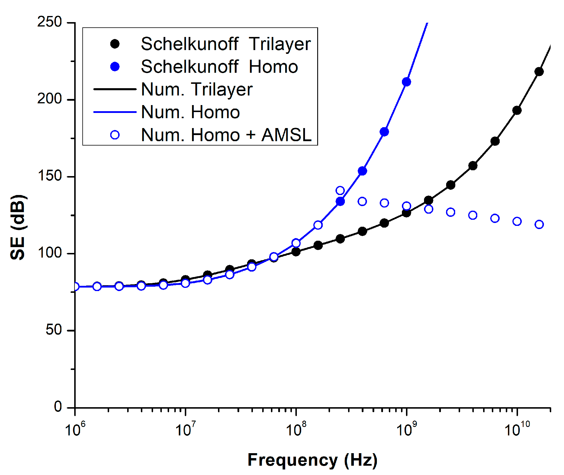
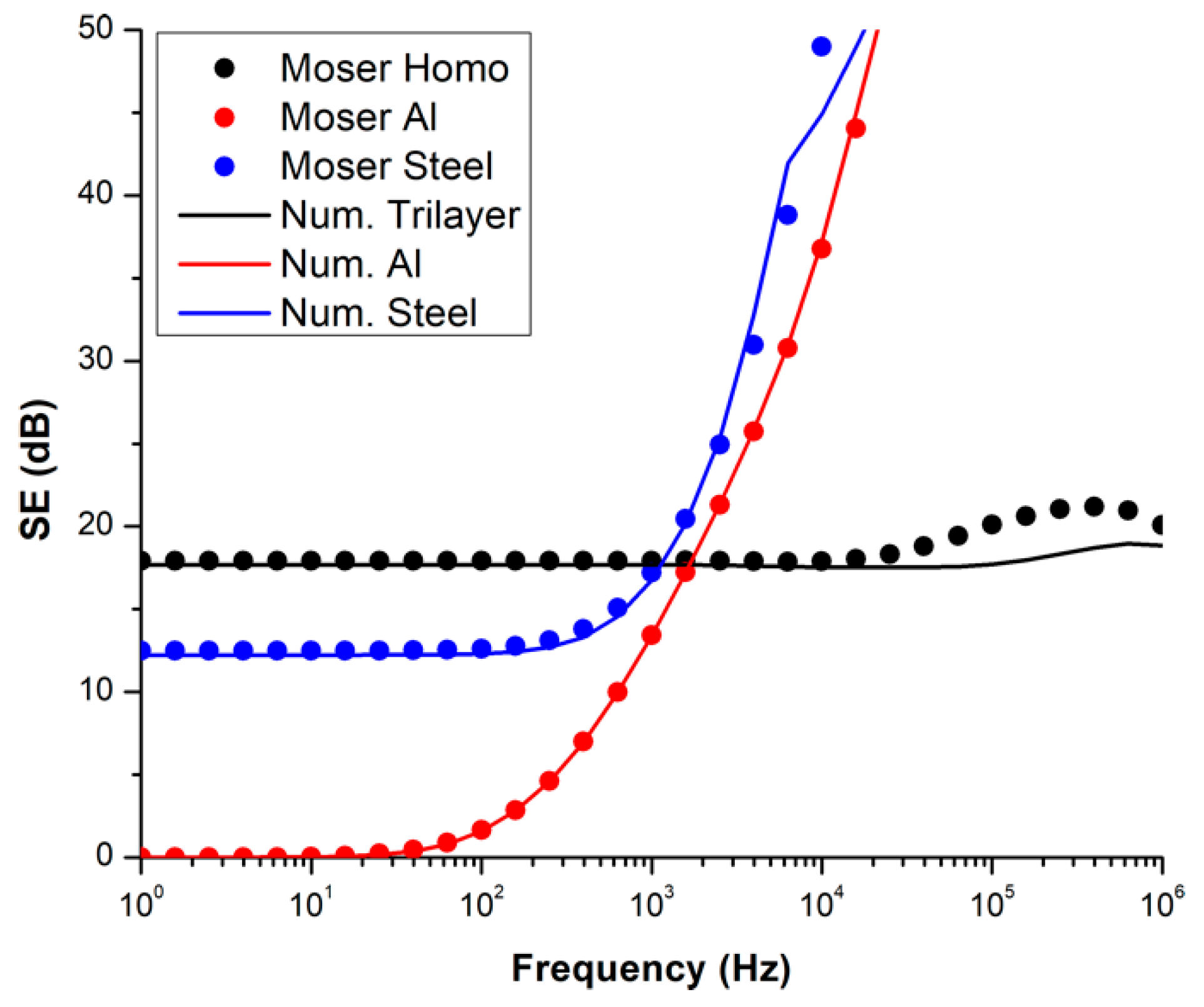
3.4. Validity of Homogenization and AMSL Methods
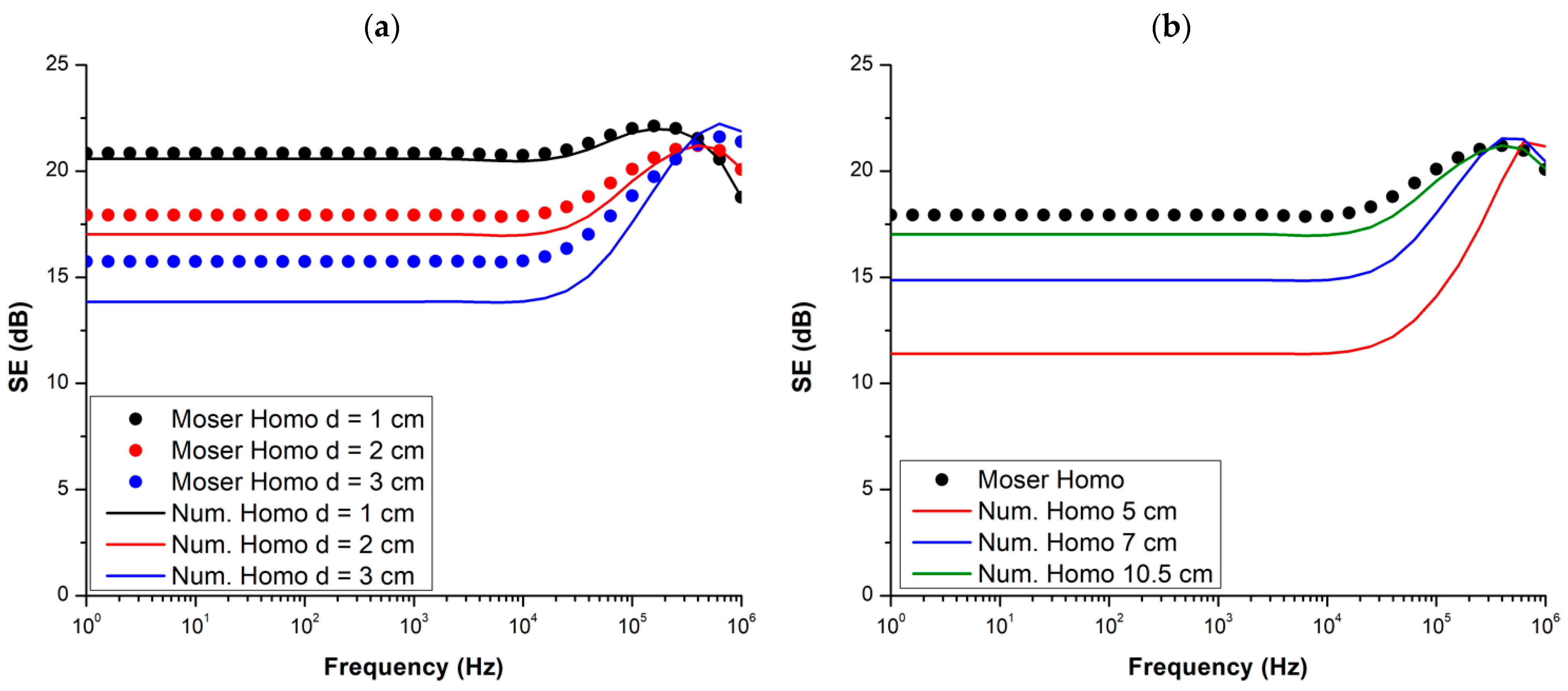
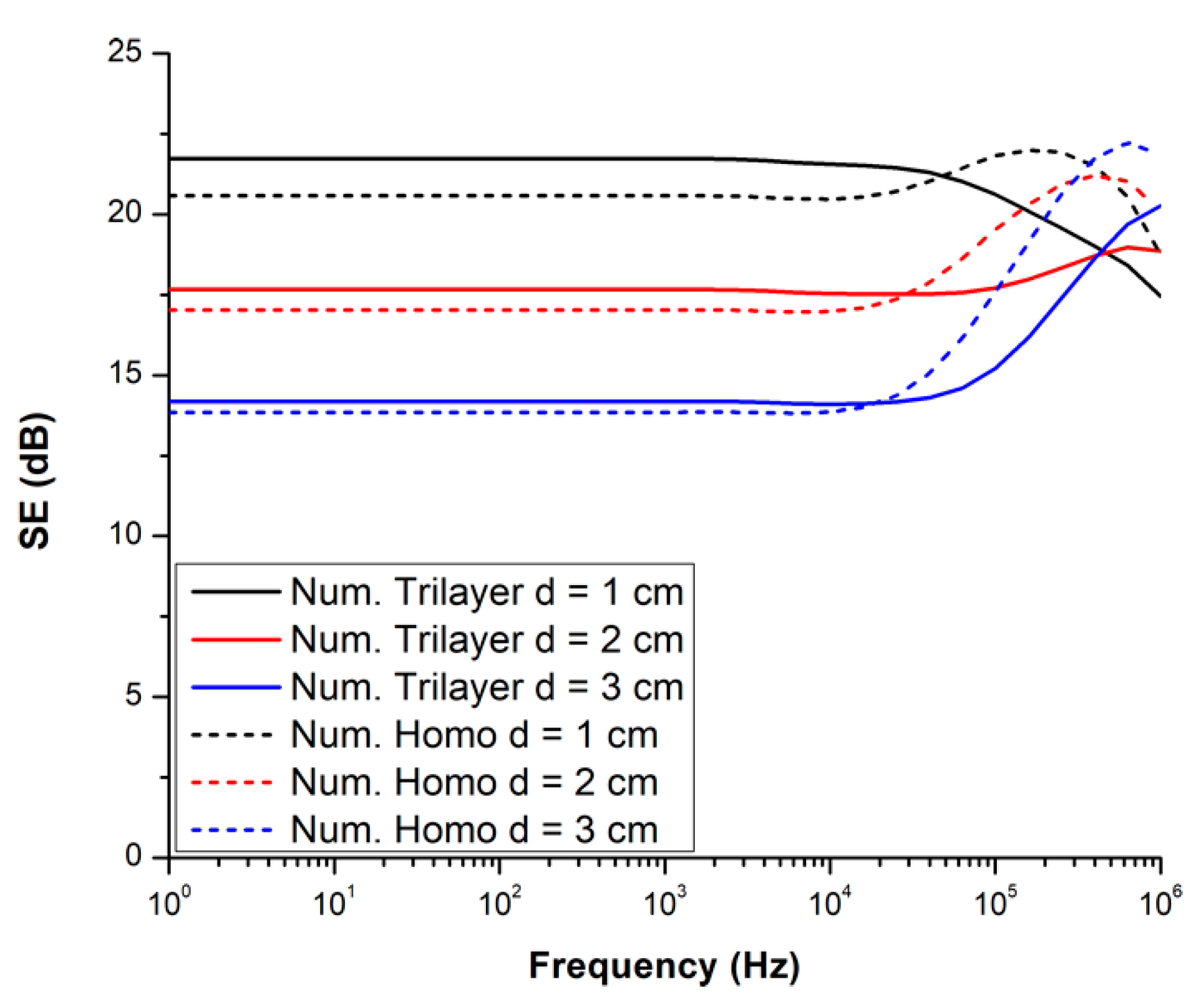
3.5. Iso-Mass Study
4. Conclusions
Author Contributions
Funding
Conflicts of Interest
References
- Chen, X.; Liu, L.; Liu, J.; Pan, F. Microstructure, electromagnetic shielding effectiveness, and mechanical properties of Mg-Zn-Y-Zr alloys. Mater. Des. 2015, 65, 360–369. [Google Scholar] [CrossRef]
- Park, J.; Lee, J.W.; Choi, H.J.; Jang, W.G.; Kim, T.S.; Suh, D.S.; Jeong, H.Y.; Chang, S.Y.; Roh, J.C.; Yoo, C.S.; et al. Electromagnetic interference shielding effectiveness of sputtered NiFe/Cu multi-layer thin film at high frequencies. Thin Solid Films 2019, 677, 130–136. [Google Scholar] [CrossRef]
- Matsuzawa, S.; Kojima, T.; Mizuno, K.; Kagawa, K.; Wakamatsu, A. Electromagnetic simulation of low-frequency magnetic shielding of a welded steel plate. IEEE Trans. Electromagn. Compat. 2021, 63, 1896–1903. [Google Scholar] [CrossRef]
- Arellano, Y.; Hunt, A.; Haas, O.C.L. Evaluation of near-field electromagnetic shielding effectiveness at low frequencies. IEEE Sens. J. 2019, 19, 121–128. [Google Scholar] [CrossRef]
- Joo, K.; Lee, K.J.; Sung, H.J.; Seung, J.L.; Jeong, S.Y.; Park, H.H.; Kim, Y.H. Evaluation of package-level EMI shielding using conformally coated conductive and magnetic materials in low and high frequencies range. In Proceedings of the 2020 IEEE 70th Electronic Components and Technology Conference (ECTC), Orlando, FL, USA, 3–30 June 2020; pp. 647–652. [Google Scholar] [CrossRef]
- Clérico, P.; Mininger, X.; Prévond, L.; Baudin, T.; Herlbert, A.-L. Compromise between magnetic shielding and mechanical strength of thin Al/steel/Al sandwiches produced by cold roll bonding: Experimental and numerical approaches. J. Alloys Compd. 2019, 798, 67–81. [Google Scholar] [CrossRef]
- Clérico, P.; Mininger, X.; Prévond, L.; Baudin, T.; Herlbert, A.-L. Magnetic shielding of a thin Al/steel/Al composite. COMPEL 2020, 39, 595–609. [Google Scholar] [CrossRef]
- Ma, X.; Zhang, Q.; Luo, Z.; Lin, X.; Wu, G. A novel structure of Ferro-Aluminum based sandwich composite for magnetic and electromagnetic interference shielding. Mater. Des. 2016, 89, 71–77. [Google Scholar] [CrossRef]
- Watanabe, A.O.; Raj, P.M.; Wong, D.; Mullapudi, R.; Tummala, R. Multilayered electromagnetic interference shielding structures for suppressing magnetic field coupling. J. Electron. Mater. 2018, 47, 5243–5250. [Google Scholar] [CrossRef]
- Nisanci, M.H.; de Paulis, F.; Di Febo, D.; Orlandi, A. Sensitivity analysis of electromagnetic transmission, reflection and absorption coefficients for biphasic composite structures. In Proceedings of the 2014 International Symposium on Electromagnetic Compatibility, Gothenburg, Sweden, 1–4 September 2014; pp. 438–443. [Google Scholar] [CrossRef]
- Liu, P.S.; Qing, H.B.; Hou, H.L.; Wang, Y.Q.; Zhang, Y.L. EMI shielding and thermal conductivity of a high porosity reticular titanium foam. Mater. Des. 2016, 92, 823–828. [Google Scholar] [CrossRef]
- Kim, S.S.; Kim, S.T.; Yoon, Y.C.; Lee, K.S. Magnetic, dielectric, and microwave absorbing properties of iron particles dispersed in rubber matrix in gigahertz frequencies. J. Appl. Phys. 2005, 97, 10F905. [Google Scholar] [CrossRef]
- Jalali, M.; Dauterstedt, S.; Michaud, A.; Wuthrich, R. Electromagnetic shielding of polymer-matrix composites with metallic nanoparticles. Compos. Part B 2011, 42, 1420–1426. [Google Scholar] [CrossRef]
- Jianzhong, W.; Jun, M.; Hao, Z.; Huiping, T. Preparation and electromagnetic shielding effectiveness of metal fibers/polymer composite. Rare Met. Mater. Eng. 2017, 46, 73–77. [Google Scholar] [CrossRef] [Green Version]
- Darques, M.; Spiegel, J.; De La Torre Medina, J.; Huynen, I.; Piraux, L. Ferromagnetic nanowire-loaded membranes for microwave electronics. J. Magn. Magn. Mater. 2009, 321, 2055–2065. [Google Scholar] [CrossRef]
- Qin, F.X.; Peng, H.X.; Pankratov, N.; Phan, M.H.; Panina, L.V. Exceptional electromagnetic interference shielding properties of ferromagnetic microwires enabled polymer composites. J. Appl. Phys. 2010, 108, 044510. [Google Scholar] [CrossRef] [Green Version]
- Xu, Y.L.; Uddin, A.; Estevez, D.; Luo, Y.; Peng, H.X.; Qin, F.X. Lightweight microwire/graphene/silicone rubber composites for efficient electromagnetic interference shielding and low microwave reflectivity. Compos. Sci. Technol. 2020, 189, 108022. [Google Scholar] [CrossRef]
- Liu, Y.; He, D.; Dubrunfaut, O.; Zhang, A.; Zhang, H.; Pichon, L.; Bai, J. Go-CNTs hybrids reinforced epoxy composites with porous structure as microwave absorbers. Compos. Sci. Technol. 2020, 200, 108450. [Google Scholar] [CrossRef]
- Fan, X.; Zhang, G.; Li, J.; Shang, Z.; Zhang, H.; Gao, Q.; Qin, J.; Shi, X. Study on foamability and electromagnetic interference shielding effectiveness of supercritical CO2 foaming epoxy/rubber/MWCNTs composite. Compos. Part A 2019, 121, 64–73. [Google Scholar] [CrossRef]
- Xie, Y.; Li, Z.; Tang, J.; Li, P.; Chen, W.; Liu, P.; Li, L.; Zheng, Z. Microwave-assisted foaming and sintering to prepare lightweight high-strength polystyrene/carbon nanotube composite foams with an ultralow percolation threshold. J. Mater. Chem. C 2021, 9, 9702–9711. [Google Scholar] [CrossRef]
- Chung, D.D.L.; Eddib, A.A. Effect of fiber lay-up configuration on the electromagnetic interference shielding effectiveness of continuous carbon fiber polymer-matrix composite. Carbon 2019, 141, 685–691. [Google Scholar] [CrossRef]
- Ameli, A.; Jung, P.U.; Park, C.B. Electrical properties and electromagnetic interference shielding effectiveness of polypropylene/carbon fiber composite foams. Carbon 2013, 60, 379–391. [Google Scholar] [CrossRef]
- Song, W.L.; Cao, M.S.; Lu, M.M.; Bi, S.; Wang, C.Y.; Liu, J.; Yuan, J.; Fan, L.Z. Flexible graphene/polymer composite films in sandwich structures for effective electromagnetic interference shielding. Carbon 2014, 66, 67–76. [Google Scholar] [CrossRef]
- Moser, J.R. Low frequency shielding of a circular loop electromagnetic field source. IEEE Trans. Electromagn. Compat. 1967, 9, 6–18. [Google Scholar] [CrossRef]
- Schelkunoff, S.A. Electromagnetic Waves; Bell Telephone Laboratories Series; Van Nostrand: New York, NY, USA, 1943. [Google Scholar]
- Kühn, M.; John, W.; Weigel, R. Analytical calculation of intrinsic shielding effectiveness for isotropic and anisotropic materials based on measured electrical parameters. Adv. Radio Sci. 2014, 12, 83–89. [Google Scholar] [CrossRef] [Green Version]
- Cruciani, S.; Campi, T.; Maradei, F.; Feliziani, M. Conductive layer modeling by improved second-order artificial material single-layer method. IEEE Trans. Antennas Propag. 2018, 66, 5646–5650. [Google Scholar] [CrossRef]
- Holland Shielding Systems BV. 2021. Available online: https://hollandshielding.com/Mu-ferro-tape-foil (accessed on 1 June 2021).


| Layer | Thickness | Conductivity (S/m) | Relative Permeability |
|---|---|---|---|
| SL (glass fiber/epoxy) | 2 mm | 1 × 10⁻¹² | 1 |
| CL (graphene) | 50 μm | 6.8 × 10⁵ | 1 |
| ML (mu-ferro) | 23 μm | 4.8 × 10⁵ | 14,200 (1 Hz) 1340 (1 MHz) 1 (>1 MHz) |
Publisher’s Note: MDPI stays neutral with regard to jurisdictional claims in published maps and institutional affiliations. |
© 2021 by the authors. Licensee MDPI, Basel, Switzerland. This article is an open access article distributed under the terms and conditions of the Creative Commons Attribution (CC BY) license (https://creativecommons.org/licenses/by/4.0/).
Share and Cite
Clérico, P.; Pichon, L.; Mininger, X.; Dubrunfaut, O.; Gannouni, C.; He, D.; Bai, J.; Prévond, L. Design of a Lightweight Multilayered Composite for DC to 20 GHz Electromagnetic Shielding. Electronics 2021, 10, 3144. https://doi.org/10.3390/electronics10243144
Clérico P, Pichon L, Mininger X, Dubrunfaut O, Gannouni C, He D, Bai J, Prévond L. Design of a Lightweight Multilayered Composite for DC to 20 GHz Electromagnetic Shielding. Electronics. 2021; 10(24):3144. https://doi.org/10.3390/electronics10243144
Chicago/Turabian StyleClérico, Paul, Lionel Pichon, Xavier Mininger, Olivier Dubrunfaut, Chadi Gannouni, Delong He, Jinbo Bai, and Laurent Prévond. 2021. "Design of a Lightweight Multilayered Composite for DC to 20 GHz Electromagnetic Shielding" Electronics 10, no. 24: 3144. https://doi.org/10.3390/electronics10243144
APA StyleClérico, P., Pichon, L., Mininger, X., Dubrunfaut, O., Gannouni, C., He, D., Bai, J., & Prévond, L. (2021). Design of a Lightweight Multilayered Composite for DC to 20 GHz Electromagnetic Shielding. Electronics, 10(24), 3144. https://doi.org/10.3390/electronics10243144