Selected Genetic Algorithms for Vehicle Routing Problem Solving

Abstract

The traveling salesman problem (TSP) consists of finding the shortest way between cities, which passes through all cities and returns to the starting point, given the distance between cities. The Vehicle Routing Problem (VRP) is the issue of defining the assumptions and limitations in mapping routes for vehicles performing certain operational activities. It is a major problem in logistics transportation. In specific areas of business, where transportation can be perceived as added value to the product, it is estimated that its optimization can lower costs up to 25% in total. The economic benefits for more open markets are a key point for VRP. This paper discusses the metaheuristics usage for solving the vehicle routing problem with special attention toward Genetic Algorithms (GAs). Metaheuristic algorithms are selected to solve the vehicle routing problem, where GA is implemented as our primary metaheuristic algorithm. GA belongs to the evolutionary algorithm (EA) family, which works on a “survival of the fittest” mechanism. This paper presents the idea of implementing different genetic operators, modified for usage with the VRP, and performs experiments to determine the best combination of genetic operators for solving the VRP and to find optimal solutions for large-scale real-life examples of the VRP.

1. Introduction

The traveling salesman problem (TSP) consists of the need to visit many places in the shortest, safest, and least expensive way and then return to the starting point, so that the route does not take too much time, wasting company resources. Usually this problem is presented with the help of a graph or map whose points are expressed by cities and the edges connecting them—roads.

This problem has a special feature—it is not possible to solve it any other way than by comparing all possible routes. This feature makes this problem NP-hard. In practice (that is, having a limited amount of available time), heuristic methods are used to solve NP-difficult problem. These methods do not guarantee finding the optimal solution but offer an acceptable approximate solution in a reasonable time. In addition to heuristic methods, which are created to solve one specific problem, there are metaheuristic methods. Their main advantage is that they can be used for more than one problem and do not require prior knowledge of the space available solutions. Most often they combine the features of random search algorithms (random search) and algorithms that use gradient navigation in the space of solutions (for example, in the hill-climbing algorithm). They demand only a measure by which it will be possible to assess how optimal the found solution so. This measure usually has the form of a polynomial function value, whose arguments belong to the searched solution space.

The Vehicle Routing Problem (VRP) is a generic name given to a set of problems in which a set of routes for a fleet of vehicles based on one or several depots are to be formed to serve the customers dispersed geographically. The objective of the VRP is to form a route with the lowest cost to serve all customers.

The vehicle routing problem is a major problem in distribution and logistics. The VRP was first described in 1959, by Dantizg and Ramser, and was called The Truck Dispatch Problem. It may be considered a more broad and generalized variation of the traveling salesman Problem [1], which has a large number of possible solutions (for 15 locations that have to be visited, there exist 15! solution, in other words, 653,837,184,000 valid and proper routes that can be created); therefore, it is difficult to determine the best and optimal solution. In the original traveling salesman problem, the optimization was performed to minimize mileage, but in modern times, values such as time or petrol usage can be also used as main optimization values, as they are usually somehow correlated with distance. VRP is a combinatorial integer programming problem [2,3], which is NP-hard [2].

There are some domains of business, with transportation regarded as added value to the product, where the optimization of vehicle routing can lower costs up to 25% in total [4]. The economic benefits of more open markets are a key point for VRP. In addition, current technology makes it possible to use VRP solutions in more a dynamic environment, working from live data and performing calculations in realtime [5].

This paper discusses the usage of genetic algorithms for the vehicle routing problem. The genetic algorithm, as an algorithm of natural selection, searches space for an approximate solution to problems with multiple solutions. One of the applications is the search for the optimal path; here, it is a more complex problem, as the limitations of route selection defined in the VRP problem are imposed. The paper analyzes the influence of genetic operators on the efficiency of the algorithm, demonstrating their influence on the search for a solution.

The idea is to find the solution to the NP-hard vehicle routing problem with the use of metaheuristics. The chosen metaheuristic was a genetic algorithm, that belongs to the group of evolutionary strategies as a part of Artificial Intelligence. The paper presents the analysis of metaheuristics usage for solving the vehicle routing problem with special attention toward genetic algorithms. The created prototype implements different genetic operators, modified for usage with vehicle routing problem. Set experiment series were performed to determine which combination of genetic operators is best for solving vehicle routing problem, to determine how much participation certain genetic operators should have in the process of producing results for the vehicle routing problem, and finally, which one will enable finding the optimal solution for large-scale real-life instances of the vehicle routing problem.

The main contributions of the paper are as follows:

• First, we analyze the use of the GA along with other metaheuristic algorithms to solve the VRP. Here, a prototype modular and flexible general purpose GA is implemented.
• Second, we show the implementation of different GA operators that are modified to solve the VRP. Designing and running experiments enable determination of the best combination of genetic operators for solving the VPR.
• Third, we analyze the impact and participation of GA operators through simulations of the selected problem.
• Finally, experiments are conducted to find an optimal solution for a large-scale real-life instance of the VRP.

The paper is structured as follows: Section 2 describes the vehicle routing problem, its definition, and methods for solving the VRP. Section 3 presents the most important ideas of a genetic algorithm and its modifications for the vehicle routing problem. Section 4 discusses the implementation details of the genetic algorithm prototype to solve the vehicle routing problem with a description of five experiments run for this solution, while Section 5 presents the results of the genetic algorithm implementation for the vehicle routing problem obtained for two of the experiments: all combinations, moderate settings, fast experiment, crossover domination experiment, mutation domination experiment, and the best combinations, long, and large instances experiment.

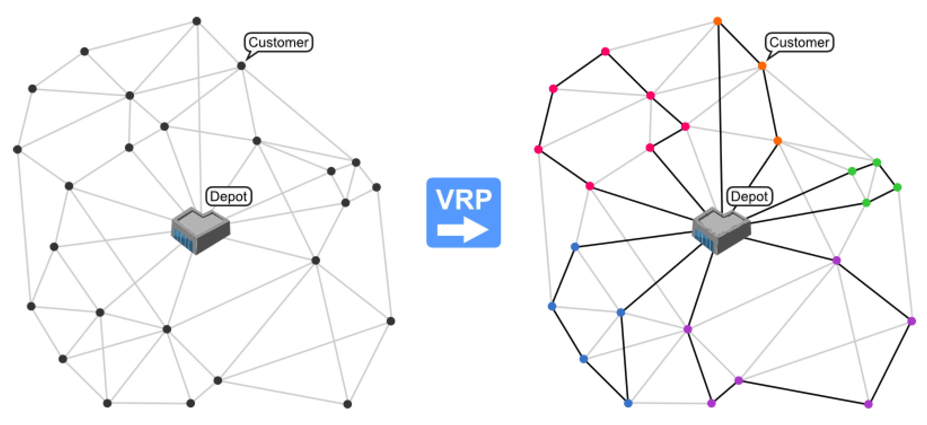
2. The Vehicle Routing Problem and Its Approach

The vehicle routing problem describes planning routes for logistics or courier companies. The most classical description would incorporate one depot location, where all vehicles within a logistic fleet start their journeys. Each of the carriers has the same capacity, and there exists a number of packages that are bound to delivery addresses. The problem that exists is how to assign packages and deliveries, so that all packages will be delivered, and the total distance covered by whole fleet will be as small as possible [6]. Figure 1 presents an instance of a VRP on the left, with its solution on the right.

2.1. Definition of a VRP

Let us assume that Q is a vector of deliveries $Q=[q_1,q_2,q_3\cdots q_n]$. Given the capacity C

$$C\ge \sum _{i=1}^n{q}_i$$

(1)

The problem is no different than the traveling salesman problem, as one entity in the fleet could take all the deliveries. Therefore, C must be bound by condition

$$C<\sum _{i=1}^n{q}_i$$

(2)

Now we describe the real VRP problem that has to be solved. The same mathematical model can be used for different sizes of carriers and different goods to be delivered to certain points. The only restriction is the one mentioned above, along with $C={\sum }_{i=1}^m{c}_i$ where $c_i$ is capacity of a single carrier in whole fleet. For simplicity, let us consider that all carriers have the same and constant capacity of c [1].

The next step is based on the idea of determining into how many stages of aggregation the problem should be divided. Each step is suboptimized, and the synthesis of these suboptimizations is the final solution to the problem [1]. Let us define an ordered sequence of deliveries $q_1,q_2,q_3\cdots q_i,q_i+1,\cdots q_n$ such that $q_i\le q_i+1$ for any $i=1,\cdots n-1$. Then t has to be determined in a way that two conditions must be met

$$C\ge \sum _{i=1}^t{q}_{i}andC<\sum _{i=1}^{t+1}{q}_i$$

(3)

t can be perceived as the representation of how many deliveries one truck can perform at maximum. The number of aggregations to be employed must take into the consideration the ordered subset of Q, which is $q_1,q_2,q_3\cdots q_t$ in the final aggregation. Obviously, such a case would take place if N, defined as the number of aggregations, is described as

$$N\approx {log}_{2}t$$

(4)

This can be derived from the fact that $2^N$ is the largest number of points aggregated in the Nth and final stage of aggregation.

Formally, the vehicle routing problem can be described as follows [1]:

• Define n points that are delivery locations $P_i(i=1,2,3\cdots n)$, define $P_0$ to represent the depot.
• Define a distance matrix that stores the distances between pairs of points $\left[D\right]=\left[d_{ij}\right](i,j=1,2,3\cdots n)$.
• Define a delivery vector that describes how many goods have to be delivered to each point $\left(Q\right)=\left(q_i\right)(i=1,2,3\cdots n)$.
• Define each single truck capacity $C>max{q}_i$.
• If $x_{ij}=x_{ji}=1$, define points $P_i,P_j$ as paired.
• If $x_{ij}=x_{ji}=0$, define points $P_i,P_j$ as not paired.
• Derive the condition

  $$\sum _{j=0}^n{x}_{ij}=1(i=1,2,3\cdots n).$$

  (5)
  Each point $P_i$ is connected with $P_0$ or at most one other point.
• By all previous definitions $x_{ij}=0$ for every $i=0,1,2\cdots n$.
• Finally, define the problem as finding such values of $x_{ij}$ that have a total distance

  $$D=\sum _{i,j=0}^n{d}_{ij}{x}_{ij}$$

  (6)

  where D is minimum, given all the conditions specified above.

2.2. Methods for Solving the VRP

Since the first formulation of the problem of optimal vehicle routing, there have been many algorithms designed to solve it. The first type of algorithm (i.e., exact) was focused on finding the best solution among all available, which becomes problematic with a large number of knots in the illustrative graph problem. The second kind of algorithm (metaheuristic and heuristic) tried to find a “good enough” solution in an acceptable time. In addition, they adapted themselves well to the changing conditions of the problem, and therefore, are widely used in dynamic route planning. Heuristic algorithms are designed for a specific problem, which is why using them on a wider scale is limited. In addition, they tend to “get stuck” in the local optimum, while exploring the crawl space. In contrast, metaheuristic algorithms work at a higher level of abstraction and are not susceptible to the aforementioned problem, due to the fact that they search the solution space to a much greater extent.

Heuristic methods are focused primarily on finding a solution within the allowed time. This may not be optimal, but it is good enough–further improvement solutions may be temporarily inefficient. They are capable of finding a relatively good solution in a short period of time, although a very limited solution space is being explored. The heuristic approach known as constructive methods builds a solution that meets given constraints, while the costs of the operation are limited and observed [7,8,9]. Such an approach does not explicitly contain a phase where improvement is made. Algorithms such as: Matching Based [10,11], Clark Furthermore, Wright [12] or Multi-Route Improvement Heuristics [13,14,15] are used in that approach.

Finally, decomposition of a problem into two phases, known as a 2-phase algorithm has been performed–with division into two separate sub-problems: clustering vertices and route construction. Two main groups of such algorithms exist, depending on which subtask is to be performed first [16,17]: Cluster-First, Route-Second Algorithms and Route-First, Cluster-Second Algorithms.

As an NP-hard problem, a classical deterministic approach can lead to complex and time-consuming computations, which poses many algorithmic challenges. It is natural to search for fast and scalable solutions to solve such a problem with the use of optimizing metaheuristics, as a function can be naturally formed for the whole problem. There exist several metaheuristics than can be used to solve the VRP, some of which are:

• Simulated Annealing—a method which mimics the metallurgical process of cooling a batch of smithed ingot slowly. A value called temperature is defined that is being evolved during a single run, moving to a minimum. The temperature value is used to escape local minimal values; when the temperature rises, the algorithm selects a worse solution; it then moves away from a local minimum valley to search in the maximum possible search area. A modification known as Deterministic Annealing has produced good results in the VRP problem, where a decision to choose a worse solution is made, based on deterministic threshold calculations, rather than random number generator results [18,19]. In [20], they propose a violation of constraints for a penalty in an objective function.
• Ant algorithms—that is, based on observation of how ant colonies establish routes around their nest. Artificial ant objects are introduced into the VRP, and each moving ant leaves behind a pheromone trail that encourages other ants to move using the same route. There should at least as many ants, as there are customers, for the algorithm to work efficiently [11,21]. In [11], a nearest-neighbour heuristic with probabilistic rules was proposed. Two colonies that cooperate in updating the best solution are proposed to minimize the number of vehicles and total distance.
• Tabu Search—can be described as a metaheuristic that is instituted on another heuristic. The Tabu search explores space by moving from one solution to its neighbours. There may exist a situation where all neighbours are worse than the currently chosen solution, and to prevent the algorithm from coming back to a stronger position that was recently considered as best, the idea of forbidden, or tabu, moves is introduced. Such actions have the capacity of introducing a larger error, but also can gain a better solution, as declaring tabu moves encourages the algorithm to visit more solutions, thus expanding the search area [11]. In [22], Li and Lim present a new approach to insertion and an extended sweep heuristic to simulated annealing with elements of a tabu search.
• Genetic Algorithms—group of well known metaheuristics that mimic biological Darwinian evolution. Solutions are randomly chosen from a group of all possible solutions, and then by modifications, known as genetic operators, they are transformed to create the next generation of solutions. Evaluation is performed on every iteration of the algorithm (meaning, every time a generation is created) and stops after the initially set termination event (number of generations, the solution being good enough, etc.) [2,8,23,24]. In [25], they proposed an evolutionary search based on mutation—each offspring is optimized to improve the total distance by using a local search and route elimination.
• Particle Swarm Optimization, PSO—was designed by Kennedy and Eberhart [26]. This method imitates swarm behavior such as fish schooling and bird flocking. Bird can find food and share this information with others. Therefore, birds flock into a promising position or region for food and this information is shared, and other birds will likely move into this location. The PSO imitates bird behavior by using a population called swarm. Each member in the group is a particle. Each particle finds a solution to the problem. Thus, position sharing of experience or information takes place and the particles update their positions and search for the solution themselves [27]. Similar constraints were found in [28,29,30] even taking in consideration the weight and size of the cargo, as we see in [31].

2.3. Genetic Algorithm Comparison with Other Algorithms

Particle Swarm is similar to a genetic algorithm in that it creates a population or in this case a swarm of possible solutions at each iteration. Each solution or particle in the swarm has a direction and a velocity. At each iteration the movement of the particle is determined by a mixture of the directions in which it is currently moving. The direction of the best point is found in the past, which is the direction the whole swarm has discovered. The idea is that more and more particles will eventually move towards areas where better solutions are found and that the swarm will eventually converge on the optimal value [32]. Analyzing these algorithms, the following commonalities can be distinguished:

• PSO and GA are both population-based stochastic optimization.
• Both algorithms start with a randomly generated population.
• Both algorithms have fitness values to evaluate the population.
• PSO and GA update the population and search for the optimum with random techniques.
• Both algorithms do not guarantee success.

As for differences:

• PSO does not use genetic operators, such as crossover and mutation. Particles update themselves with internal velocity.
• Particles also have memory, which is important to the algorithm.

  -

  Not “what” that best solution was, but “where” that best solution was.

• Particles do not die.
• The information sharing mechanism in PSO is significantly different.

  -

  The information moves from best to others, where the GA population moves together.

The vehicle routing problem can also be solved using Tabu Search (TS). Tabu search is based on introducing flexible memory structures in conjunction with strategic restrictions and aspiration levels as a means for exploring search spaces. It is a metaheuristic that guides a local heuristic search procedure to explore the solution space beyond local optimum by use of a Tabu list. It is used to solve combinatorial (finite solution set) optimization problems by a dynamic neighborhood search method. It uses a flexible memory to restrict the next solution choice to some subset of neighborhood of the current solution [33]. The main advantage of TS over GA is the use of its memorized approach, which prevents the algorithm from searching for the solution in previously visited areas. Therefore, TS has an ability to easily escape from a local optimum and find a global optimum in a shorter time [34].

3. Genetic Algorithm and Its Modifications for the Vehicle Routing Problem

Work on evolutionary systems, of which genetic algorithms are part, began in the 1950s. In the 1960s, Rechenberg introduced the idea of evolution strategies, and Fogels, Walsh and Owens developed the first evolution programming working example. Based on these inventions, Holland with a group of other researchers from the University of Michigan developed in the 1960s and 1970s the idea of genetic algorithms (GA) [35]. In contrast to research on evolutionary programming, Holland’s idea was to explore the general idea of adaptation based on natural observations and find a way to incorporate that knowledge in machine processing. It was proposed as a randomized global search technique based on natural evolution [36].

Originally, GA was a method that takes a population of problem solutions, represented as a binary string, and transforms the whole population to another one by a set of modifications inspired by Darwinian natural selection. These operators were selection, reproduction, and mutation. Selection ensured that the strongest individuals, understood as better solutions, have a larger probability to produce offspring. Offspring on the other hand were generated by reproduction, that took the form of crossing parts of one solutions with parts of another one. Finally, randomized mutation was introduced, usually in the form of swapping two bits or negating just one of them in an individual in the whole population. Holland’s model not only described the idea but was theoretically proven and is still used today as a starting point for all modern genetic algorithms [37].

The classical approach to genetic algorithms is not valid for sequential problems such as the traveling salesman problem or the vehicle routing problem. The main problem is that a single solution cannot be represented as a set of bits. The proper encoding of a solution is a string of integer numbers, representing vertices of a problem-space graph [4].

3.1. Representation of VRP Solution for Genetic Algorithm

Number 0 represents a starting point in a graph, or in other words, a depot in a real life. Clients or delivery points are assigned an integer number from 1 to n, where n is the number of deliveries to be performed. Cars in the fleet are assigned to the numbers from n + 1 to m − 1. Obviously the quantity of the vehicles in a fleet is equal to m − n, but one truck is always skipped. Given all of the above, the proper solution can be constructed in modular manner. A string of integers is built with as many blocks as there are vehicles performing the task. The basic structure of a single module consists of an integer assigned to the vehicle and two zeroes, as each routes starts and ends in the depot. Each customer’s number that is being serviced by that vehicle is placed in between the zeroes, in order of the delivery. All modules are put together to create a final solution representation. Zeroes can be removed to increase readability. An exception exists, as the first module in the whole representation does not need to have a vehicle representing an integer in the first position. After that operation, if two integers representing vehicles are adjacent to each other, or a string ends with such an integer, that means that not all vehicles take part in the solution, and can be safely removed too, if all vehicles have the same capacity. Figure 2 shows a proper way to encode the solution to the VRP with 10 deliveries and 4 trucks.

3.2. Selection

Selection is a step where the population part that will be reproduced and alive in next step is chosen. Generally, the only formal requirement that has to be met is the fact that the fittest individuals must have a higher probability of being chosen. Some examples of possible selection methods are [37]:

• Roulette wheel selection (RWS)—chances of an individual being chosen are proportional to its fitness value; thus, selection may be imagined as a spinning roulette, where each individual takes an amount of space on the roulette wheel according to its fitness.
• Elitism selection (ES)—a certain percentage of the population, ordered by fitness, is always transferred to the next population. In that scenario, the algorithm makes sure that best so far known solutions would not be lost in the process of selection.
• Rank selection (RS)—similar to RWS, but each individual solution’s space on the roulette wheel is not proportional to its fitness, but to its rank in the list of all individuals, ordered by fitness.
• Stochastic universal sampling selection (SUSS)—instead of spinning the wheel of the roulette for a certain amount of times, spin it once. If selecting n individuals, there must exist n spaces on the wheel, and the chosen individual is copied n times to the next generation.
• Tournament selection (TS)—as many times as required, choose two individuals randomly, and let the more fit one be chosen.

3.3. Crossover Operators

With the change in chromosome representation, all genetic operators must be adjusted accordingly. Firstly, simple crossover operators that incorporate swapping parts of two parent chromosomes to produce offspring no longer suffice for the needs of the new representation [4]. Figure 3 shows the problem.

Swapping parts of a chromosome can introduce unwanted pathology in the form of doubling delivery points or trucks. Such a solution can be automatically marked as invalid. There exist many different solutions to that problem, but this paper only focus on the simple solution derived from crossover operators for TSP, as VRP is nothing else than generalized version of a problem described in the literature as the traveling salesman problem.

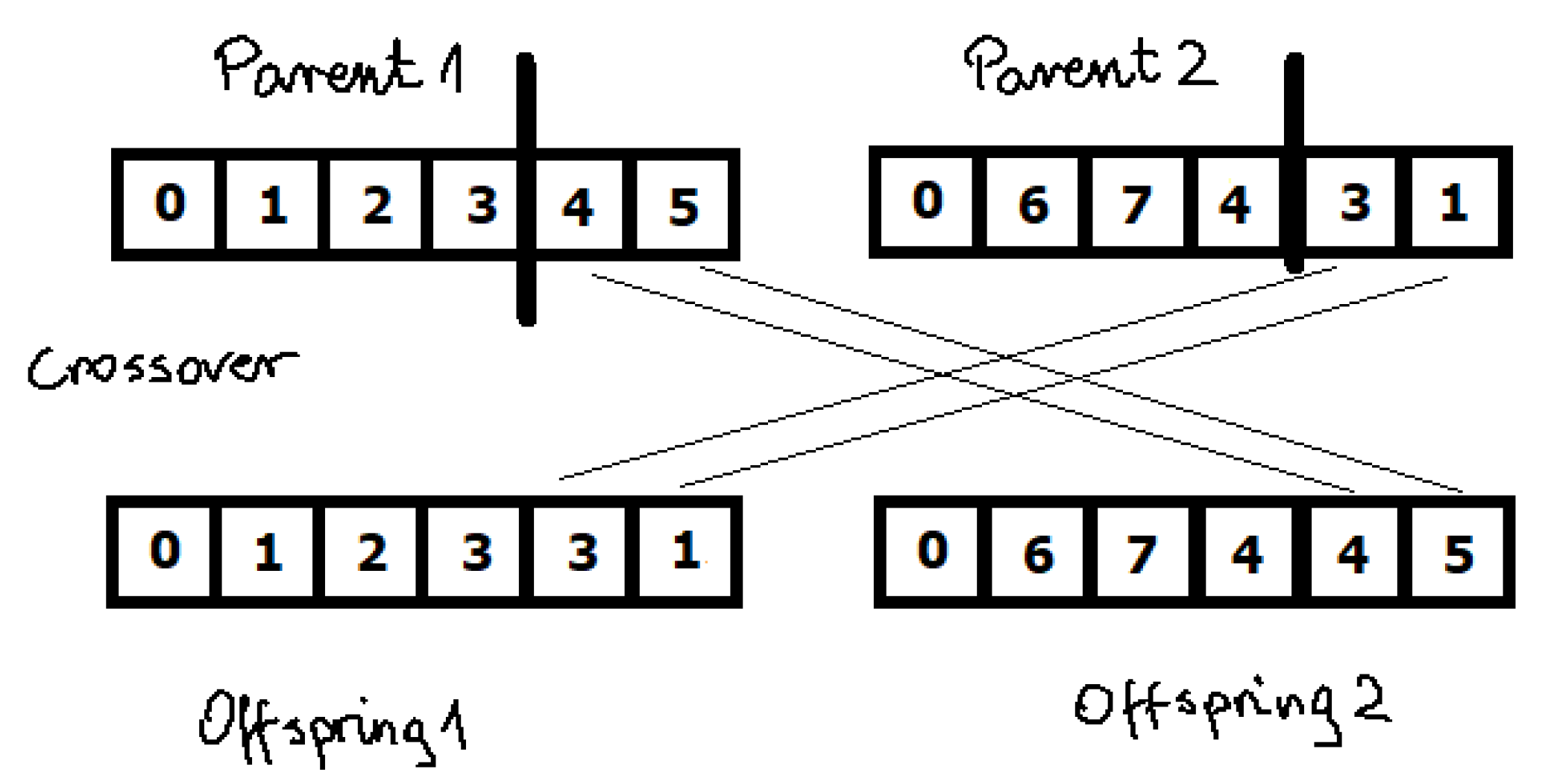
3.3.1. Order Crossover

One of the most simple, yet effective ideas for TSP crossover [38,39] is order crossover, and its variation for the VRP [40,41] is presented in Figure 4. To perform order crossover, certain actions have to be taken:

• Label parents randomly as male and female.
• Take both parents and randomly choose two crossover points, the same for both of them.
• Copy the integers in between the crossover points, from male parent to child, keeping them at the same positions.
• Take the female parent, and starting from the gene after the second crossover point, iterate through all genes. If the end is met, start from the beginning.
• Take the child and starting from the gene after the second crossover point, copy the female parent gene that is considered in the current iteration, only if it is not present yet in the child’s chromosome. If the end is met, start from the beginning.
• The operation is finished if all empty spaces in the child chromosome are filled.
• Optionally, swap the roles of female and male parents, and repeat the whole process to produce a second offspring.

Such a simple technique enables creation of valid chromosomes for the next population, where the order of the parent’s vertices is preserved [42].

3.3.2. Partially Mapped Crossover

Start the same as order crossover, with choosing two crossing points and copying part of the first parent to the new child.

Then, to preserve as much order as possible from the second parent, integers that are not included in the part copied from first parent are inherited from second one, together with their positions.

3.3.3. Edge Recombination Crossover

This is based on the idea of randomly inheriting as many parent’s edges as possible, promoting edges that are common for both parents, by introducing the idea of neighborhood. For each integer in the representation, a neighborhood vector can be created, by choosing vertices that are adjacent to this integer in both parents’ representations.

3.3.4. Cycle Crossover

Cycle crossover performs two operations for copying a single element. First, the element itself is chosen from one parent, then the element’s position in the child is determined by the element’s position in the other parent. One parent is always used to determine the choice of elements, and the other one is always responsible for position choices. Let us assume parents $p1$ and $p2$. The process starts with copying the first element from $p1$ to the first position of the child, then, a loop starts. In the loop, from $p2$, the first integer is nominated, but it is copied to the child in the fourth position, as this is the position it takes in $p1$. Then, in $p2$, integer 8 is nominated, as it lies in position four, but it is copied to the child in position eight, as in $p1$,

3.4. Mutation Operator Changes in Regard to Integer Solution Representation

Mutation operators do not need to be completely reinvented. Swap mutation is still valid, but instead of swapping two bits, two integer values are swapped in the entire solution. It does not matter what these values represented, it is safe to mutate by swapping location and vehicle integers [4]. The negation mutator can be replaced by a very similar remove-and-reinsert operation, as shown in Figure 5.

The idea behind this kind of mutation is simple. Take a vertex at a certain position, reduce its representation size, and randomly place it in another spot, restoring the original size.

It is worth noting at this point that it is believed that simple mutation operators should act as a secondary entropy source in the algorithm and not provide as many perturbations to produce competitive results as compared to other techniques. Based on that fact, hybrid genetic algorithms have been designed that incorporate local search methods that act as mutation operators. Hybrid genetic algorithms are beyond the scope of this paper, but some of them worth mentioning introduce a local descent [43] or Tabu search [44].

3.5. Related Works on Genetic Algorithm and the Vehicle Routing Problem

One of the first works presenting a genetic algorithm to solve the VRP with a time window was [45]. The author described a genetic algorithm heuristic, named GIDEON, for solving the VRPTW (vehicle routing problem with time windows). GIDEON consisted of two methods: global customer clustering and local post-optimization. The global customer clustering method used an adaptive search strategy based upon population genetics to assign vehicles to customers. The second method was used to improve the best solution obtained from the clustering method.

The first effective implementation of the genetic algorithm for VRPTW was proposed by [46]. The authors described the GENEtic ROUting System (GENEROUS), which was based on a natural evolution paradigm. Using this paradigm, a population of solutions evolved from one generation to the next to form new offspring solutions, with the use of “mating” parent solutions, that exhibited characteristics inherited from the parents. The specialized methodology was devised for merging two vehicle routing solutions into a single solution that was likely to be feasible with respect to the time window constraints.

Many other papers presented different modifications of genetic algorithms, especially with different versions of the select, cross, and mutation operators. The authors of [47] considered a combined objective Capacitated Vehicle Routing Problem (CVRP) as a combinatorial optimization problem in which a fleet of vehicles with limits on capacity were available to service a set of customers from a central depot with their individual demands known in advance. To solve this problem a Genetic Algorithm technique was used by two different crossovers to enhance the quality of generated solutions. The proposed model was validated using the information obtained from a distribution company.

Recently, a hybrid solution using metaheuristics and heuristic or adopting the GA for new variants of the VRP was proposed.

The authors of [48] considered the optimization of the Capacitated Vehicle Routing Problem with Alternative Delivery, Pickup, and Time windows. This problem was presented based on postal and courier delivery issues as a combination of many variants of the classical VRP, such as CVRP, VRPTW, and VRPPD (Vehicle Routing Problem with Pickup and Delivery). However, the presented problem introduced alternative delivery points and parcel lockers incorporated into the distribution network and the ability to take into account logical constraints. It was formulated in the form of BIP (Binary Integer Programming) with integration of CP (Constraint Programming), GA (Genetic Algorithm), and MP (Mathematical Programming) to implement and optimize the model.

Euchi and Sadok [49] proposed a hybrid approach to improve the combination of sweep and genetic algorithms to solve the VRPD (VRD with drones) problem. A MILP (mixed integer linear programing) model was presented to describe the problem, and it was formulated via CPLEX software with small examples. The experiments were carried out on examples taken from the literature in different settings.

Ongcunaruk et al. [50] proposed improving the transportation planning decisions for a production company by a collaborative decision routing model for a logistics provider and food manufacturer. The authors formulated the mixed integer programming model to minimize a cost function, which consists of fixed vehicle costs, variable vehicle costs, and fuel costs. To approximate the optimal solution, the genetic algorithm (GA) was developed. Moreover, a partial factorial design of GA parameters was implemented to determine the suitable parameter values to guide the genetic algorithm.

The authors of [51] proposed using the Big Data frameworks to solve an optimization of the Dynamic Vehicle Routing Problem (DVRP). They developed a parallel Spark Genetic Algorithm to take the advantage of Spark’s in-memory computing ability and GA’s iterations operations. Based on the parallel S-GA, a decision support system was developed for the DVRP in order to generate the best routes. The realized experiments showed that the proposed architecture was improved due to its capacity.

He et al. [52] considered the Yard crane (YC) scheduling problem with the uncertainty of task groups’ arriving times and handling volumes. They optimized the efficiency of YC operations. Furthermore, a mathematical model was proposed to optimize the total delay to the estimated ending time of all task groups. Moreover, the GA-based framework combined with a three-stage algorithm was proposed to solve the problem, together with numerical experiments.

4. Implementation of Genetic Algorithm to Solve the Vehicle Routing Problem

The key point during implementation of the genetic algorithm to solve the vehicle routing problem was to provide as much modularity as possible. Therefore, the core of the genetic algorithm is a completely separate module that is written in such a way that it can be used not only to solve VRP problems but any problem feasible for GA solutions [53,54,55].

Another modular component is chromosome representation. Objects representing chromosomes are of a class that implements all mutation operators for them. Such an approach provides encapsulation of all logic related to the genome and operations performed on it. The last required module is a goal function calculating mechanism. The algorithm must be seeded with the following parameters:

• initial population size,
• amount of population that will be transferred to the next population,
• amount of population transferred, which is allowed to reproduce,
• amount of population transferred, which is allowed to mutate,
• number of generations after which the algorithm will terminate itself, and
• the class name representing the chromosome with its genetic operators.

Population parts that are transferred, mutated, and crossed-over must all together equal the initial population size, in each generation. All additional parameters, such as vehicle count, their capacity, locations with coordinates, and the quantity of goods that needs to be delivered are provided as additional parameters and usually are passed to the algorithm in the third module, together with the fitness function, as almost only that function makes use of them.

4.1. Vehicle Routing Problem Test Instances

In order to obtain comparable results, all experiments were performed on well-known and described test examples. The choice of examples was made to ensure variety and to cover the usually chosen test examples for all the experiments. Six main groups of examples were chosen:

• Augerat Set A—described by the Augerat team in 1995 [56], set A consists of 27 examples that were generated randomly. Points are randomly spread across a 100 × 100 square, with demand in each point usually around 15. Demand is chosen in a uniform manner, and 10% of all coordinates have their demand tripled. Capacity for a single vehicle is always 100.
• Augerat Set B—described by the Augerat team in 1995 [56], set B consists of 23 examples, created in a way, such that coordinates are randomly spread but joined together in n clusters, and n is always larger than number of available vehicles. Demand is randomly distributed from 1 to 30, with 10% of all places to visit having their demand tripled.
• Augerat Set P—described by the Augerat team in 1995 [56] is a set of modified examples previously known in the literature.
• Christofides and Eilon Set E—described in the literature in 1969 [57], which contains 13 examples, with coordinates always spread uniformly in the search space.
• Fisher Set F—a set of three, real life problems, used by Fisher in their work [9]. Two are days of grocery deliveries from the Peterboro (Ontario terminal) of National Grocers Limited, and the third one is generated based on data obtained from Exxon associated with the delivery of tires, batteries, and accessories to gasoline service stations.
• TSPLIB converted Ulysses instances—two classic examples, converted to a VRP problem from TSPLIB, which is a library of traveling salesman problem examples. Both chosen ones were based on the mythical journey that Ulysses took, represented on a map.

All examples are sets of coordinates, meaning that they take place in euclidean two-dimensional space, with only vertices given. No cost of traveling through graph edges is provided, and only distance counts. The examples were used in standard format, containing example settings, and coordinate data.

4.2. Design of Experiments for the Genetic Algorithm in the Vehicle Routing Problem

One of the aims was to determined how the genetic operator percentage usage on population affected the results, how the combinations of selections with crossover operators behaved, and finally, how well a properly scaled genetic algorithm instance can perform in large-scale real life instances; hence, a few different experiments had to be performed.

4.2.1. All Combinations, Moderate Settings, Fast Experiment (AcMsF)

The initial experiment aim was to observe how combinations of selection and crossover operator behaved in situations, when a balanced small population was reproduced for fairly short number of iterations. This will enable observing the behavior of all combinations, nominating promising ones for later experiments, and seeing how close each of them converged to the optimal result.

To provide a wide variety of instances, all the Ulysses and Fisher examples were used. From sets A, B, P, and E, the smallest, largest, and moderate in size examples were chosen. This provided 17 examples, on each of which 20 combinations of selection and crossover operators were performed, resulting in total 340 GA runs. The population was always 100, of which 40% was kept alive, 10% was mutated, and 50% was crossed-over. All runs were performed for 1000 generations. It was suspected that for smaller examples, some reasonable results would be presented, but the short duration of time given would not produce any good results for larger examples.

4.2.2. All Combinations, Moderate Settings, Long Experiment (AcMsL)

In this experiment, large populations of individuals were enabled to reproduce for an extended number of generations. The aim of this experiment was to examine how combinations of operators perform close to the maximum efficiency. The best results from this experiment would surely be described as the strongest possible combinations, and therefore, would be used in later experiments.

Similar to the previous experiment, 17 examples were chosen, 340 runs were performed. The population structure stayed the same, but the algorithm would be allowed to terminate after ten times more iterations.

4.2.3. Crossover Domination Experiment (CD)

This experiment was designed to determine if crossover alone was sufficient and would produce reasonable results. This time, from each set A, B, P, and E, two moderate in size examples were used. That way, repetitiveness would be forced.

The three top performing combinations from previous experiments were used. The algorithm ran for 1000, 5000, and 10,000 generations, population sizes were 100, 500, and 1000, with only 10% of the population copied, and 90% crossed-over. It is believed that the crossover operator should be strong enough alone to provide good results, but lack of mutation may lead to slower convergence to optimal results in the first thousand iterations.

4.2.4. Mutation Domination Experiment (MD)

This experiment was designed to determine if mutation alone was sufficient and would produce reasonable results. As above, from each set A, B, P, and E, two moderate in size examples were used. That way, repetitiveness would be forced.

Only the remove-and-reinsert mutation was used. The algorithm ran for 1000, 5000, and 10,000 generations, population sizes were 100, 500, and 1000, with only 10% of the population copied, 5% crossed-over, and 85% mutated. Fast increase in fitness in early iterations should be observed, due to the enormous entropy of the whole system, but mutation alone should not be sufficient to converge to satisfying results, no matter how much time was given.

4.2.5. Best Combinations, Long, Large Examples Experiment (BcLBi)

This final experiment was to test whether the proposed implementation of the genetic algorithm was capable of reaching the top results, very close to optimal ones, in case of the largest data sets. The most important instance here, was the Fisher 135 nodes example, as this was a certified real life instance, that mostly reassembled what difficulties would face a VRP solving system in everyday use. The largest examples from all sets were also used.

The optimal template of the population structure was used, with around 30% to 40% of individuals being copied over. The rest was determined, based on the two previous experiments. Three top performing crossover-selection combinations were used. The algorithm was terminated after 20,000–30,000, with a population count of 10,000. At least one result should be close to the optimal value of the Fisher instance. We also observed how the results compared to the ones from the first two experiments, to state how convergence changed based on the size of the population and number of iterations.

Table 1. Experiments for the genetic algorithm in the vehicle routing problem.

Experiment	Large Examples	Medium Examples	Small Examples	Total Instances	Combinations	Populations	Generations
AcMsF	5	5	7	17	20	100	1000
AcMsL	5	5	7	17	20	500	10,000
CD	0	8	0	8	3	100, 500, 1000	1000, 5000, 10,000
MD	0	8	0	8	1	100, 500, 1000	1000, 5000, 10,000
BcLBi	5	0	0	5	3	10,000	25,000

sums up all the experiments that were performed.

5. Results of the Genetic Algorithm Implementation for the Vehicle Routing Problem

This section presents the results of selected cases of the genetic algorithm implementation for the vehicle routing problem:

• The all combinations, moderate settings, fast experiment;
• The crossover domination experiment;
• The mutation domination experiment;
• And the best combinations, long, large examples experiment.

The optimal value is known for all instances. All settings, optimal value, distance of the best found solution from that optimum and the representation of the best fitted individual are presented. Distance was calculated such that solutions worse than the best-known have a negative number. If in any case the algorithm found a better fitted individual, its distance would was a positive floating point number.

How far a solution was from an optimal one could not be analyzed, as traveled distances differ for each instance and are dependent on large amount of constraints written into them, introduced during the generation process. With that in mind, all the results analyzed were percentage values of how far from the best-known result the algorithm was. The equation used to compute these values is as follows:

$$v=\frac{f\ast 100\%}{o}-100\%$$

(7)

where v is value calculated in percent, f is the best value found in a single run by the GA, and o is the optimal solution fitness value for the example that was used in the GA run.

5.1. All Combinations, Moderate Settings, Fast Experiment

In this experiment, to cut computation time as much as possible and observe how well all combinations of the used selection and cross-over operators behaved with hard constraints, populations of one hundred individuals were allowed to reproduce for one thousand generations. In each of them, half were copied over, four-tenths were allowed to reproduce, and one tenth were mutated. Such settings provided stressful conditions for reproduction and were used to observe, how fast each combination, and the genetic algorithm in general, started to approach optimal results.

A wide selection of examples brought as much variety as possible. The examples used were:

• Small examples:

  -

  Augerat, Set A, 32 deliveries, 5 vehicles,

  -

  Augerat, Set B, 32 deliveries, 5 vehicles,

  -

  Augerat, Set P, 35 deliveries, 5 vehicles,

  -

  Christophides and Eilon, Set E, 22 deliveries, 4 vehicles,

  -

  Fisher, Set F, 45 deliveries, 4 vehicles,

  -

  Ulysses, Set U, 16 deliveries, 3 vehicles,

  -

  Ulysses, Set U, 22 deliveries, 4 vehicles.

• Medium examples:

  -

  Augerat, Set A, 55 deliveries, 9 vehicles,

  -

  Augerat, Set B, 57 deliveries, 9 vehicles,

  -

  Augerat, Set P, 57 deliveries, 5 vehicles,

  -

  Christophides and Eilon, Set E, 51 deliveries, 5 vehicles,

  -

  Fisher, Set F, 72 deliveries, 4 vehicles.

• Large examples:

  -

  Augerat, Set A, 80 deliveries, 10 vehicles,

  -

  Augerat, Set B, 78 deliveries, 10 vehicles,

  -

  Augerat, Set P, 78 deliveries, 10 vehicles,

  -

  Christophides and Eilon, Set E, 101 deliveries, 14 vehicles,

  -

  Fisher, Set F, 135 deliveries, 7 vehicles.

Given the above choices, seventeen instances were chosen, with all twenty possible combinations, resulting in three hundred and forty GA runs.

5.1.1. Averaged Results for All Combinations

Table 2. All combinations, moderate settings, fast experiment–averaged results from all instances from first experiment.

	Elitism	Rank	Roulette	Tournament
alternating_edges_crossover	78.98%	67.81%	78.18%	69.53%
cycle_crossover	52.20%	49.87%	47.36%	48.57%
edge_recombination_crossover	79.53%	80.18%	82.40%	77.13%
order_crossover	49.31%	50.12%	50.78%	45.76%
partially_mapped_crossover	46.76%	42.28%	48.73%	43.63%

shows the averaged data gathered for all combinations, from all instances.

What is very interesting is the fact that all cross-over methods working on vertices, rather than whole edges, generated better results. To be precise, in no case, alternating edges crossover and edge recombination crossover, produced averaged results lower than 69%, while the other three crossovers never exceeded the averaged result of 53%. To investigate this matter more closely, it seems reasonable to analyze the data with regard to the size of the used examples. Let us divide the examples used as described in the list representing examples for the experiment, grouping by small, medium, and large labels.

Table 3. All combinations, moderate settings, fast experiment—averaged results for small, medium, large, and all instances, grouped by crossover methods.

	Small	Medium	Large	All
alternating_edges_crossover	14.69%	74.92%	142.79%	73.62%
cycle_crossover	20.41%	49.72%	84.13%	49.50%
edge_recombination_crossover	12.88%	82.42%	157.00%	79.81%
order_crossover	20.26%	50.68%	81.43%	48.99%
partially_mapped_crossover	19.04%	49.95%	71.40%	45.35%

shows the averaged data divided into these groups, for each crossover technique.

The column All in Table 3 reinforces the data from Table 2. Crossovers that incorporated working on edges rather than vertices, performed worse compared to others. This can be explained by their results for the large examples, which were far above 100%. Surprisingly, when analyzing the data, which was generated by running GA on smaller examples, it can be observed that edge crossovers performed better than ones working on single vertices. The reason behind such behavior is possibly the limited amount of generations, during which evolution was performed, so for smaller instances, less time was required to start observing stable optimization in the global minimum well of search space. That would mean that edge-based operators need more time, and they are far more superior to vertex-based ones in long less constrained calculations. In the first generations, it is important to produce enough entropy, so that individuals can spread roughly throughout the whole search space. Vertex-based crossovers, possibly generate more entropy, as they do not pay attention to edge inheritance, resulting in more random offspring during reproduction. Backed up with mutation, they start finding optimal solutions faster, but that amount of entropy does not allow them to produce satisfying results in the long run. On the other hand, edge-based methods spread throughout the search space in a slower manner, but when approaching extremum, it is easier for them to actually reach it, as less randomization provides more stability and control for the optimization process. It can be also observed, that partially mapped crossover performed very well, and should be used in cases when it is unknown or hard to estimate how much time is required to reach satisfying results.

In

Table 4. All combinations, moderate settings, fast experiment—averaged results for small, medium, large, and all instances, grouped by selection methods.

	Small	Medium	Large	All
elitism	16.85%	63.87%	111.74%	61.36%
rank	18.97%	58.05%	104.95%	58.05%
roulette	16.87%	66.18%	109.40%	61.49%
tournament	17.14%	58.05%	103.31%	56.92%

, averaged results for small, medium, large, and all instances are grouped by selection methods. Here, differences were smaller, in general, selection methods differed at most by no more than 7%, and in case of the averaged data from all instances the difference was no larger than 5%. It may be observed that despite small differences, the tournament selection was best. If a decision was to be made, the tournament selection should be chosen, but rank selection also behaved quite well.

5.1.2. Graphical Representation of Results and Best Found Solutions

Firstly, the global average calculated from all the results in this experiment was equal to 59.55% and could not be by any means considered as satisfying and optimal. Solutions that had combined routes path larger than the currently known best ones, were still usually, when plotted, random and unsatisfactory. To illustrate this, Figure 6 represents the plotted solution that had almost the same distance from the optimal solution as on average. The used combination was a partially mapped crossover with elitism, performed on a middle sized, Christophides&Ellion example from set E.

The x and y axes enabled specifying the x/y coordinates of individual points of the generated routes. The lines presented in different colors represent different routes generated by different algorithms during the realization of experiments.

It can be seen, that as mentioned, the solution looks slightly random, with routes intersecting one another many times. From a more optimistic perspective, round-shaped routes started to appear, meaning that the algorithm started the optimization process and the solution was not completely bad. In the first generations, as starting population have only random solutions, not all vehicles are usually used and paths are jagged, with a possibility of a route going from one end to the other. Such bad solutions can be observed in larger examples in this experiment, because of the fact that, for many of them, one thousand generations was not enough to even start finding more properly organized routes. An example of such a situation was one of the worst obtained results, also from the Christophides and Ellion example from set E. This time, edge recombination was used with rank selection, and the solution was as far from the optimal one as 172% (Figure 7).

This jagged pattern without even proper routes starting to form can be seen in almost all results from large examples. On the other hand, the experiment was designed in a way to still provide the ability to achieve good results. In such a short time it is hard, but not impossible to achieve good results, varying no more than 5% from the best known one. The high factor describing the amount of population being copied over can ensure that such solution would be carried over through the generations to the end of GA run. It basically counts on luck, and can be suspected in smaller instances, as the probability of randomly constructing a good initial genome is higher if there are fewer variables. It actually happened quite often, given the constraints, to obtain solutions below 10% of the distance from optimal ones, but there is one lucky exception found in the results from the mentioned set E. Figure 8 shows the solution from the smallest Christophides&Ellion example, only 3.2% worse than the best one.

5.2. Crossover Domination Experiment

The crossover domination experiment was designed to check how well the dominant crossover genetic operator could behave in comparison to experiments with more restrained and balanced settings. Although the part of the population that was crossed over was actually 85%, still 10% of the best individuals were copied over throughout all generations. Additionally, mutation was present, although only 5% of the population was allowed to mutate.

Originally, the experiment was designed in a way that no mutation would be present at all, but the results from such altered GA runs were catastrophically bad, as even during longer runs, the algorithm was usually not capable of reaching any reasonable results at all. Lack of mutation in any form made it unable to descend into proper fitness function minimal values, resulting in the crossover operator looking for results near the starting random positions. The results were distant in percentages of more than a couple thousand from the optimal solution. That indicated that the spread throughout the search space was so minimal that path sequences were not fulfilling the capacity constraint, as the fitness function could produce such wrong results only when the penalty function started to take a dominant place in the final fitness of individuals. Figure 9 presents such an individual, seemingly a completely random solution, despite ten thousand iterations performed on a population from which this best one was chosen.

Selected instances for the experiment were all medium sized, chosen from sets that were created by random set distribution. From each of these sets two such examples were chosen. The complete list of instances used in this experiment was as follows:

• Augerat, Set A, 45 deliveries, 7 vehicles,
• Augerat, Set A, 54 deliveries, 7 vehicles,
• Augerat, Set B, 45 deliveries, 6 vehicles,
• Augerat, Set B, 56 deliveries, 7 vehicles,
• Augerat, Set P, 45 deliveries, 6 vehicles,
• Augerat, Set P, 56 deliveries, 7 vehicles,
• Christophides and Eilon, Set E, 33 deliveries, 4 vehicles,
• Christophides and Eilon, Set E, 51 deliveries, 5 vehicles.

Based on previous experiments, the three best performing on the long run combinations of selection and crossover operators were nominated and used:

• alternating edges crossover with rank selection,
• alternating edges crossover with tournament selection,
• edge recombination crossover with tournament selection,

Each combination was run on each instance for three times to emulate different lengths of GA runs, for 1000 generations with 100 population size, 5000 generations with 500 population size, and 10,000 generations with 1000 population size. These resulted in 72 GA runs.

5.2.1. Averaged Results for Crossover Domination

Table 5. Crossover domination experiment—averaged results from all examples, grouped by population sizes and iterations count.

Size	Generations	Average Distance
100	1000	56.05%
500	5000	17.48%
1000	10000	12.57%

contains the data from the crossover domination experiment, averaged and grouped by population sizes and iterations performed.

For shorter runs, the average result was at the same level as the results from the first experiment. Increasing population size and allowing the algorithm to work for longer periods of time caused the results to become dramatically better. That means that dominant crossover, with just a small amount of entropy generated by mutation operator is capable of finding very competitive results. At first, the improvement was linear. However, it must be pointed out that when the algorithm descended below the threshold of 20% distance from best known solutions, the improvement with each increase in computational resources began to be less and less noticeable. That relationship can be observed in Figure 10, where the average result is plotted with regard to the resources assigned to the algorithm.

Reinforcing the data gathered in previous experiments, alternating edges crossover with rank selection seemed to be the strongest combination, producing the best individuals, as represented in

Table 6. Crossover domination experiment—averaged results from all instances, grouped by crossover and selection.

Crossover	Selection	Average Distance
alternating_edges	rank	26.06%
alternating_edges	tournament	27.28%
edge_recombination	tournament	32.76%

.

The global average for the whole experiment was equal to 28.7%, but when runs with 100 population size and 1000 iterations were removed from the calculations, the global difference from the world optimal results dropped to 15% and was lower than the medium examples average from experiment two, which equaled 18.6%. Allowing individuals to reproduce, and ensuring that their offspring take a majority of space in the next generation can help improve the final results.

5.2.2. Graphical Representation of Results and Best Found Solutions

As mentioned, excluding the shortest runs from the calculation produced an average fitness value of the best individuals around 15% worse than the globally best solution. Such results can be regarded as good. Figure 11 presents the plotted solution for the Christophides and Eilon, Set E examples, distant by 15.43% from the optimum. Such a solution can be used to represent the average individual for the whole experiment.

The same situation as in experiment two occurred. It can be expected from such promising results to find at least a few very good solutions. There were 17 solutions with distance from the best ones no larger than 10%. There were again two exceptional ones, both from Christophides and Eilon, Set E, smaller examples that had a fitness closer than 1% to the best one. They are presented in Figure 12 and Figure 13.

5.3. Mutation Domination Experiment

As discussed in the previous experiment, lack of mutation makes the genetic algorithm unable to descend into proper solutions, but mutation alone, as a dominant operator, could not produce competitive results, compared to the situation when most of the population was copied and crossed-over. To determine if that was actually true, this experiment was designed. Analyzing the results from both the crossover domination and mutation domination experiment will enable to see the difference between usage of these two operators in terms of solving the VRP.

The design of the experiment was from one point of view similar to the previous one, as exactly the same examples, population sizes, and generation counts were used. The only changed part was the symmetrical swap in the percentage of the population being reproduced and mutated. Now, 85% of the population was mutated each iteration and only 5% allowed to produce offspring. As crossover played a minimal role, only one combination, alternating edges crossover with rank selection was used, reducing the global run count to 24.

5.3.1. Averaged Results for Mutation Domination

Table 7. Mutation domination experiment—averaged results from all instances, grouped by population sizes and iterations count.

Size	Generations	Average Distance
100	1000	34.51%
500	5000	24.01%
1000	10,000	13.09%

presents the averaged data gathered from all examples, grouped by generation count and population size. When mutation had precedence above crossover, the relation between the averaged results settings of the genetic algorithm became perfectly linear. It was suspected that the line in a plot in Figure 14 would eventually flatten out, but in the measured area the relation was slowly but steadily decreasing.

Table 8. Mutation domination experiment—averaged results from all examples, grouped by instance sets.

Instance	Average Distance
set A	18.34%
set B	22.13%
set P	24.17%
set E	25.73%

shows the average results from the examples, grouped by example sets. What is interesting, from set E, smaller examples were chosen than from the other ones, but the results were worse. The difference lies in the placement of the depot and locations to visit, as set E instances tend to group them. Hence, the mutation operator performed better and could help to find good results faster, if the VRP instance destinations were spread more uniformly throughout the space rather than clustered in subgroups.

The general average fitness from the whole mutation domination experiments equalled 23.9%, and it was roughly on the same level as the one from the second experiment. It has to be noted that the average result from the second experiment was highly affected by the results from the small examples, and for medium-only examples was higher for about 10%, equaling 34.8%. However, the best crossover operator, the edge recombination crossover, had an average in small examples from experiment two as low as 18%. Therefore, mutation performed better than the majority of crossovers, but when the settings were chosen reasonably, more stable solutions were still better than the mutation domination.

5.3.2. Graphical Representation of Results and Best Found Solutions

With a larger amount of population carried to the next generations with the use of mutation operator, GA was capable of producing only two results that were worse than 7% from the world’s best individuals. As suspected, both were obtained by running instances for ten thousand generations. Figure 15 shows the plotted paths for an individual from the Augerat set A example with fitness values worse than the globally known optimum by 6.75%.

The result seemed to be well formed. However, two major flaws can be spotted. The right blue path was convoluted, and there was a weak, small, circular purple route, which could be used to visit some of the points from the right side of the area, therefore, making it easier to visit all of them by three not two paths. In Figure 16, the solution from a smaller Christophides and Eilon, Set E example can be observed. The fitness was worse from the optimal one by 6.38%. Clearly, three out of four paths could be optimized further, as they intersected one another.

5.4. Comparison of Mutation and Crossover Domination

After two experiments, testing the domination of two different genetic operators, it can be seen that the dominance of either one of them produced reasonable but not the best possible solutions. While major mutated populations descended in a more linear manner, it can be suspected that the function describing the best fitted average individual would flatten out, and both experiments would end with little improvement, when granted significantly greater computational resources. The linear part of the descent was just starting with better solutions at the beginning and in the case of the mutation domination had not yet reached the plateau. Figure 17 shows the two plots from both experiments side by side.

It has to be pointed out that on longer runs, crossover domination provided better solutions than GA runs performed with relatively large numbers of examples from experiment 2. Such a situation hints that a slight boost to the number of crossover offspring in the population structure could improve the results. This knowledge was used in the last, fifth, experiment. The mutated population count was not increased, as data observed in the third experiment led to the conclusion that even minimal participation of mutation products in upcoming generations was enough to spread solutions through the search space, to enable crossover methods to start descending into wells of the search space, where the minimal values of the fitness function were. The main idea, when setting up operator proportions for the VRP solving genetic algorithm, should revolve around providing enough time for the stability from the combined crossover and mutation to reach satisfying solutions. After that, repetition should be forced to increase the probability of finding exceptional individuals, as still a factor of luck counts towards achieving genomes with path meshes very close to or even better than the worldwide best-known current solutions.

5.5. Best Combinations, Long, Large Examples Experiment

The last experiment, using all the knowledge from previous ones was used to check how good a result could be obtained on the largest examples from all the sets, except Ulysses. The examples chosen for this experiment were:

• Augerat, Set A, 80 deliveries, 10 vehicles,
• Augerat, Set B, 78 deliveries, 10 vehicles,
• Augerat, Set P, 78 deliveries, 10 vehicles,
• Christophides and Eilon, Set E, 101 deliveries, 14 vehicles,
• Fisher, Set F, 135 deliveries, 7 vehicles.

The Fisher instance is the most interesting one, not only because of its size but also the fact that it is based on a real life problem, that the VRP algorithms have to solve everyday if used commercially. The other difficulty in the Fisher example is that it is very much constrained. Firstly, many destinations are clustered around the depot, and a minority is far from it. Secondly, the example makes use of relatively small fleet, so there is very little room for error, as the capacities of each vehicle in the fleet are used close to the maximum.

All instances ran three times, with three selection and crossover combinations:

• alternating edges crossover with rank selection,
• alternating edges crossover with tournament selection,
• edge recombination crossover with tournament selection.

The alternating edges crossover/rank selection combination was supposed to produce the best results, as its prominence was shown in all previous experiments. The algorithm was run with a population size of one thousand, and it was allowed to reproduce for twenty five thousand iterations. The alive structure of the generation would be altered, with 40% of individuals being copied over, 10% mutated, and 50% coming to the population as offspring from crossover reproduction. The genetic algorithm was run fifteen times.

5.5.1. Averaged Results for Mutation Domination

The general average from all fifteen runs was equal to 14.76%, which was a very good improvement compared to almost 37% average results for the larger examples from experiment two. The full results from the fifth experiment are gathered together and shown in

Table 9. Best combinations, long, large examples experiment–results for all combinations, from all instances.

Instance Type	Instance Size	Crossover	Selection	Result
set A	n80k10	alternating_edges	rank	12.16%
set A	n80k10	alternating_edge	tournament	12.52%
set A	n80k10	edge_recombination	tournament	18.76%
set B	n78k10	alternating_edges	rank	7.13%
set B	n78k10	alternating_edges	tournament	7.52%
set B	n78k10	edge_recombination	tournament	6.64%
set P	n78k10	alternating_edges	rank	7.33%
set P	n78k10	alternating_edges	tournament	13.48%
set P	n78k10	edge_recombination	tournament	31.17%
set E	n101k14	alternating_edges	rank	10.49%
set E	n101k14	alternating_edges	tournament	11.30%
set E	n101k14	edge_recombination	tournament	9.36%
set F	n135k7	alternating_edges	rank	25.51%
set F	n135k7	alternating_edges	tournament	26.18%
set F	n135k7	edge_recombination	tournament	21.96%

.

Unfortunately, the results for the Fisher example were no less than 20% from the best-known solutions for this set of destinations. This means that real life instances are difficult to explore and need even more computational power to establish good solutions. The times required for the genetic algorithm implementation to compute such large examples were around a few hours, which is too long to consider everyday use of it, as a working method of establishing routes. On smaller, randomly distributed test cases, the algorithm was capable of finding good results. In general, the alternating edges crossover with rank selection produced the best solutions in a stable manner, as seen in

Table 10. Best combinations, long, large instances experiment—averaged data from all instances, grouped by selection and crossover combinations.

Crossover	Selection	Average Distance
alternating_edges	rank	12.52%
alternating_edges	tournament	14.20%
edge_recombination	tournament	17.58%

. The edge recombination technique seemed to be a more varying method, as it produced both the best and worst individuals. Using edge recombination is therefore considered as a kind of gamble, as luck is a variable in obtaining good results. The method generally descend in a similar manner but behaves in more unpredictable way than alternating edges.

5.5.2. Graphical Representation of Results and Best Found Solutions

As many as one third of the results in this experiment had the best fitted individuals with fitness values closer to best known solution than 10%. The best results were obtained for the Augerat set B example. In Figure 18, the plot for the solution obtained with alternating edges crossover and rank selection combination can be observed. The paths are not intersecting themselves, but intersections between different routes still occur. The algorithm has roughly properly clustered the space and divided it for different vehicles. In Figure 19, an even better solution can be seen plotted. The difference in results is less than 1%, but here, a clear division for western and eastern routes can be seen. There are less intersections, and the algorithm tries to optimize by including smaller paths in larger ones. It is surprising that the best results were obtained for this instance, as intuitively, the set E largest example was much simpler, with a roughly uniform spread of destination throughout the whole task area. In the example from set B, the largest optimization problem came from the fact of three groups, tightly packed together in small areas. As seen, proper paths for them were found, but the capacity constraints made it hard to further improve the results, leaving the path to far destinations not entirely well optimized.

Christophides and Eilon’s largest example is a graceful one to optimize, as uniform spread should result in all paths having different directions. Its plot should look like a flower pattern. The best result in this experiment was 9% worse than optimal, shown in Figure 20 and can be considered good but not very good. Most of the difficulties were present in the south-west and north-east part of the space, where routes intersected badly. The rightmost yellow route was also badly optimized, as the furthest points visited by the vehicle traveling that way, should be split, and some of them should belong to green route. It can be said that a flower-like pattern started to appear, but there certainly was room for improvement.

Finally, in the last Figure 21, the best fitted individual for the Fisher largest example is graphically presented. The fitness is distant from the best one by around 22%. The same problems as in the Augerat set B example can be seen. The algorithm coped well with the tricky high density area around the depot. However, paths leading to the far left-side destinations were optimized badly. Due to the large distances that have to be covered to reach them, worse optimization on these areas led to not very competitive results.

6. Discussion and Conclusions

The genetic algorithm seemed to be a good choice for solving the vehicle routing problem. The results revealed that GA converged to the global optimum quickly, which reduced the cost of computation. It was noted that selection operators, searching operators, along with chromosome representation had an impact in finding the global solution without getting trapped at a local optimum. The results revealed that a large domination of either of the genetic operators was not positive for the final results. In general, for the VRP and possibly other problems that revolve around finding paths in large graphs, operators that pay attention to whole edges rather than single vertexes are far more superior. It was noted that GA is capable of finding good results for large examples of the VRP. However, instances based on real life problems tended to be less trivial than randomly generated ones, and for them, the GA needs to be altered or modified to provide competitive solutions.

The results of the AcMsF (“All combinations, moderate settings, fast experiment”) experiment are summarized as follows:

• Vertex-based crossovers provide higher entropy, therefore perform better in short runs.
• Edge-based crossovers perform better, when given enough time. relative to instance size.
• Selection method does not seem to impact final results very much.
• If any selection method were to be chosen, tournament would be the one, as it provides slightly better results than rest.
• The average solution is not optimal but not completely random.
• Better results were obtained in case of smaller examples.
• One thousand iterations is definitely not enough for the GA to even start producing non-random solutions for larger examples.
• Despite harsh conditions for the algorithm, it was still able to find a very optimal solution for one of the examples.

The results of the CD (“Crossover domination”) experiment are summarized as follows:

• Making crossover a dominating genetic operator provides reasonable results.
• Complete lack of mutation results in very bad individuals.
• In general, when the algorithm is run with enough computational resources, more dominant crossover provides better individuals, than more dominant best individuals’ copying.
• With tight constraints, crossover domination behaves as badly as more stable approaches.
• When crossover is dominant, at some point the algorithm starts to rapidly descend and find good representatives, but after that rapid inflation process, further improvement is slow.

The results of the MD (“Mutation domination”) experiment are summarized as follows:

• Making mutation a dominating genetic operator provides reasonable results.
• Mutation alone cannot provide results as well as a properly adjusted more stable run with edge crossover.
• Mutation behaves well, when the example has a uniform distribution of destinations.
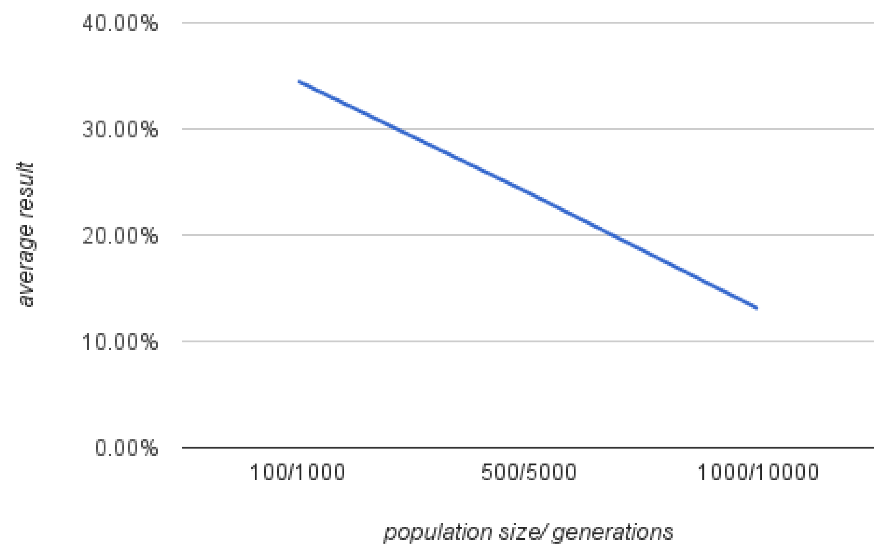
• On a smaller scale, assigning more computational resources results in a linear decrease in the average results.
• It is recommended to use slightly higher amounts of mutated offspring in the first iteration of the algorithm, as mutation is better than any type of crossover in spreading solutions across the search area.

The results of the BcLBi (“Best combinations, long, large examples experiment”) experiment are summarized as follows:

• Reasonably chosen genetic algorithm parameters can provide enough stability to start reaching satisfying results even for large examples.
• Real life instances pose greater difficulties compared to randomly distributed ones.
• Given enough time and computational power, genetic algorithm implementation can produce competitive results even in the largest known test instances.
• Optimizations of paths in areas with higher density is easier and appears earlier in the whole optimization process than optimization of routes leading to further points of interest.
• Alternating edges crossover combined with rank selection is the most stable choice for genetic operators, capable of finding results comparable with the worldwide best-known ones.

The experiment results concluded that large domination of neither of the genetic operators was positive for the final results. In general, for the vehicle routing problem and possibly other problems that revolve around finding paths in large graphs, operators that pay attention to whole edges rather than single vertexes were far more superior. The algorithm was capable of finding good results for large examples of the vehicle routing problem. However, instances based on real life problems tended to be less trivial than randomly generated ones and for them, the algorithm needs to be altered or modified to provide competitive solutions.

Without any modifications to the implementation, experiments could be run multiple times again, possibly for extended amounts of iterations. Promising results from executed runs are an indicator that more close to optimal or even better solutions can be possibly found. However, this task revolves around luck, as the function of best fitted individual through generations flattens dramatically.

The fitness function and instances representation could be altered to enable capability of testing examples that are not only based on euclidean two-dimensional space but also, for example, on explicit graph representation with weights. With costs of journey from one point to another, additional crossover operators from group of heuristic crossovers could be implemented and used. The fitness function and genetic operators could be modified to enable testing of other vehicle routing problem variants such as ones with time windows or split delivery.

One interesting area of further study is combining genetic algorithms with other techniques that partially or totally solve the vehicle routing problem. Such hybrid algorithms can be based on many different ideas:

• Simple cooperation with clustering methods for initial routes and then running independent genetic algorithms for each cluster in order to find proper routes on smaller scale,
• Hybrid usage of deterministic or heuristic methods incorporated to aid the genetic algorithm in finding better individuals,
• Exchanging parts of the genetic algorithm, especially mutation with, for example, local search methods, as mentioned in Section 2,
• Combining the work of the genetic algorithm with other metaheuristics, such as Tabu Search or Deterministic Annealing.

References

1. Dantzig, G.B.; Ramser, R.H. The Truck Dispatching Problem. Manag. Sci. 1959, 6, 80–91. [Google Scholar] [CrossRef]
2. Alba, E.; Dorronsoro, B. Solving the Vehicle Routing Problem by Using Cellular Genetic Algorithms. In Lecture Notes in Computer Science, Proceedings of the Conference on Evolutionary Computation in Combinatorial Optimization, LNCS, Coimbra, Portugal, 5–7 April 2004; Springer: Berlin/Heidelberg, Germnay, 2004; Volume 3004, pp. 11–20. [Google Scholar]
3. Vaira, G. Genetic Algorithm for Vehicle Routing Problem. Ph.D. Thesis, Vilnus University, Vilnius, Lithuania, 2014. [Google Scholar]
4. Toth, P.; Vigo, D. The Vehicle Routing Problem. In Monographs on Discrete Mathematics and Applications; SIAM: Philadelphia, PA, USA, 2001. [Google Scholar]
5. Bianchi, L. Notes on Dynamic Vehicle Routing—The State of Art. Technical Report; IDSIA-05-01; IDSIA: Lugano, Switzerland, 2000. [Google Scholar]
6. Vehicle Routing Problem. Available online: http://neo.lcc.uma.es/vrp/vehicle-routing-problem/ (accessed on 30 September 2021).
7. Tasan, A.S.; Gen, M. A genetic algorithm based approach to vehicle routing problem with simultaneous pick-up and deliveries. Comput. Ind. Eng. 2012, 62, 755–761. [Google Scholar] [CrossRef]
8. Sharma, D.; Pal, S.; Sahay, A.; Kumar, P.; Agarwal, G.; Vignesh, K. Local Search Heuristics-Based Genetic Algorithm for Capacitated Vehicle Routing Problem. In Advances in Computational Methods in Manufacturing; Lecture Notes on Multidisciplinary Industrial Engineering; Narayanan, R., Joshi, S., Dixit, U., Eds.; Springer: Berlin/Heidelberg, Germany, 2019. [Google Scholar]
9. Fisher, M.L. Optimal Solution of Vehicle Routing Problems Using Minimum K-trees. Oper. Res. 1994, 42, 626–642. [Google Scholar] [CrossRef]
10. Altinkemer, K.; Gavish, B. Parallel Savings Based Heuristic for the Delivery Problem. Oper. Res. 1991, 39, 456–469. [Google Scholar] [CrossRef]
11. Gambardella, L.M.; Taillard, E.; Agazzi, G. MACS-VRPTW: A Multiple Ant Colony System for Vehicle Routing Problems with Time Windows. In New Ideas in Optimization; Corne, D., Dorigo, M., Glover, F., Eds.; McGraw-Hill Ltd.: Maidenhead, UK, 1999; pp. 63–76. [Google Scholar]
12. Clarke, G.; Wright, J. Scheduling of vehicles from a central depot to a number of delivery points. Oper. Res. 1964, 12, 568–581. [Google Scholar] [CrossRef]
13. Thompson, P.M.; Psaraftis, H.N. Cyclic Transfer Algorithms for the Multivehicle Routing and Scheduling Problems. Oper. Res. 1993, 41, 935–946. [Google Scholar] [CrossRef]
14. Van Breedam, A. An Analysis of the Behaviour of Heuristics for the Vehicle Routing Problem for a Selection of Problems with Vehicle-Related, Customer-Related, and Time-Related Constraints. Ph.D. Thesis, University of Antwerp, Antwerp, Belgium, 1994. [Google Scholar]
15. Kinderwater, G.A.P.; Savelsbergh, M.W.P. Vehicle Routing: Handling Edge Exchanges. In Local Search in Combinatorial Optimization; Aarts, E.H.L., Lenstra, J.K., Eds.; Wiley: Chichester, UK, 1997. [Google Scholar]
16. Ryan, D.M.; Hjorring, C.; Glover, F. Extensions of the Petal Method for Vehicle Routing. J. Oper. Res. Soc. 1993, 44, 289–296. [Google Scholar] [CrossRef]
17. Taillard, A.D. Parallel Iterative Search Methods for Vehicle Routing Problems. Networks 1993, 23, 661–673. [Google Scholar] [CrossRef]
18. Dueck, G.; Scheurer, T. Threshold Accepting: A General Purpose Optimization Algorithm. J. Comput. Phys. 1990, 90, 161–175. [Google Scholar] [CrossRef]
19. Dueck, G. New Optimization Heuristics: The Great Deluge Algorithm and the Record-To-Record Travel. J. Comput. Phys. 1993, 104, 86–92. [Google Scholar] [CrossRef]
20. Chiang, W.-C.; Russell, R.A. Simulated annealing metaheuristics for the vehicle routing problem with time windows. Ann. Oper. Res. 1996, 63, 3–27. [Google Scholar] [CrossRef]
21. Bullnheimer, B.; Strauss, R.F.H.A.C. Applying the Ant System to the Vehicle Routing Problem. In Proceedings of the 2nd International Conference on Metaheuristics, Versailles, France, 21–24 July 1997. [Google Scholar]
22. Li, H.; Lim, A. Local search with annealing-like restarts to solve the VRPT. Eur. J. Oper. Res. 2003, 150, 115–127. [Google Scholar] [CrossRef]
23. Yusuf, I.; Baba, M.S.; Iksan, N. Applied Genetic Algorithm for Solving Rich VRP. Appl. Artif. Intell. 2014, 28, 957–991. [Google Scholar] [CrossRef]
24. De Oliveira da Costa, P.R.; Mauceri, S.; Carroll, P.; Pallonetto, F. A Genetic Algorithm for a Green Vehicle Routing Problem. Electron. Notes Discret. Math. 2018, 64, 65–74. [Google Scholar] [CrossRef] [Green Version]
25. Repoussis, P.P.; Tarantilis, C.D.; Ioannou, G. Arc-guided evolutionary algorithm for the vehicle routing problem with time windows. IEEE Trans. Evol. Comput. 2009, 13, 624–647. [Google Scholar] [CrossRef]
26. Kennedy, J.; Eberhart, R. Particle swarm optimization. In Proceedings of the ICNN’95—International Conference on Neural Networks, Perth, WA, Australia, 27 November–1 December 1995; IEEE: Perth, WA, Australia, 1995; Volume 4, pp. 1942–1948. [Google Scholar]
27. Anantathanavit, M.; Munlin, M. Radius Particle Swarm Optimization. In Proceedings of the 2013 International Computer Science and Engineering Conference (ICSEC), Nakhonpathom, Thailand, 4–6 September 2013; pp. 126–130. [Google Scholar]
28. Demirtas, Y.E.; Ozdemir, E.; Demirtas, U. A particle swarm optimization for the dynamic vehicle routing problem. In Proceedings of the 2015 6th International Conference on Modeling, Simulation, and Applied Optimization (ICMSAO), Istanbul, Turkey, 27–29 May 2015; pp. 1–5. [Google Scholar]
29. Lagos, C.; Guerrero, G.; Cabrera, E.; Moltedo, A.; Johnson, F.; Paredes, F. An improved Particle Swarm Optimization Algorithm for the VRP with Simultaneous Pickup and Delivery and Time Windows. IEEE Latin Am. Trans. 2018, 16, 1732–1740. [Google Scholar] [CrossRef]
30. Han, L.; Hou, H.; Yang, J.; Xie, J. E-commerce distribution vehicle routing optimization research based on genetic algorithm. In Proceedings of the 2016 International Conference on Logistics, Informatics and Service Sciences (LISS), Sydney, NSW, Australia, 24–27 July 2016; pp. 1–5. [Google Scholar]
31. Hsieh, F.-S.; Huang, H.W. Decision support for cooperative carriers based on clustering requests and discrete particle swarm optimization. In Proceedings of the 2016 IEEE Congress on Evolutionary Computation (CEC), Vancouver, BC, Canada, 24–29 July 2016; pp. 762–769. [Google Scholar]
32. Yang, C.; Guo, Z.; Liu, L. Comparison Study on Algorithms for Vehicle Routing Problem with Time Windows. In Proceedings of the 21st International Conference on Industrial Engineering and Engineering Management; Qi, E., Shen, J., Dou, R., Eds.; Atlantis Press: Paris, France, 2015; pp. 257–260. [Google Scholar]
33. Arora, T.; Gigras, Y. A survey of comparison between various metaheuristic techniques for path planning problem. Int. J. Comput. Eng. Sci. 2013, 3, 62–66. [Google Scholar]
34. Iswari, T.; Asih, A.M.S. Comparing genetic algorithm and particle swarm optimization for solving capacitated vehicle routing problem. Conf. Ser. Mater. Sci. Eng. 2018, 337, 012004. [Google Scholar] [CrossRef]
35. Mitchell, M. An Introduction to Genetic Algorithms; MIT Press: Cambridge, MA, USA, 1998. [Google Scholar]
36. Holland, J.H. Adaptation in Neural and Artificial Systems; The University of Michigan Press: Ann Arbor, MI, USA, 1975. [Google Scholar]
37. Alabsi, F.; Naoum, R. Comparison of Selection Methods and Crossover Operations using Steady State Genetic Based Intrusion Detection System. J. Emerg. Trends Comput. Inf. Sci. 2012, 3, 1053–1058. [Google Scholar]
38. Gog, A.; Chira, C. Comparative analysis of recombination operators in genetic algorithms for the traveling salesman problem. In Hybrid Artificial Intelligent Systems, Proceedings of the 6th International Conference, Part II, LNCS 6679, Wroclaw, Poland, 23–25 May 2011; Corchado, E., Kurzynski, M., Wozniak, M., Eds.; Springer: Berlin/Heidelberg, Germany, 2011; pp. 10–17. [Google Scholar]
39. Hwang, H.-S. An improved model for vehicle routing problem with time constraint based on genetic algorithm. Comput. Ind. Eng. 2002, 42, 361–369. [Google Scholar] [CrossRef]
40. Nazif, H.; Lee, L.S. Optimised crossover genetic algorithm for capacitated vehicle routing problem. Appl. Math. Model. 2012, 36, 2110–2117. [Google Scholar] [CrossRef]
41. Kumar, V.; Panneerselvam, R. A Study of Crossover Operators for Genetic Algorithms to Solve VRP and its Variants and New Sinusoidal Motion Crossover Operator. Int. J. Comput. Intell. Res. 2017, 13, 1717–1733. [Google Scholar]
42. Goldberg, D.E. Genetic Algorithms; Pearson Education: London, UK, 2006. [Google Scholar]
43. Mulhenbein, H.; Gorges-Schleuter, M.; Kramer, O. Evolution algorithms in combinatorial optimization. Parallel Comput. 1988, 7, 65–85. [Google Scholar] [CrossRef]
44. Fleurent, C.; Ferland, J.A. Genetic and hybrid algorithms for graph colouring. Ann. Oper. Res. 1996, 63, 437–461. [Google Scholar] [CrossRef]
45. Thangiah, G.D. Vehicle routing with time window using genetic algorithms. In Application Handbook of Genetic Algorithm: New Frontiers; Chambers, L., Ed.; CRC Press: New York, NY, USA, 1995; pp. 253–377. [Google Scholar]
46. Potvin, J.Y.; Bengio, S. The vehicle routing problem with time windows–Part II: Genetic search. INFORMS J. Comput. 1996, 8, 165–177. [Google Scholar] [CrossRef]
47. Mulloorakam, A.T.; Nidhiry, N.M. Combined Objective Optimization for Vehicle Routing Using Genetic Algorithm. Mater. Today Proc. 2019, 11 Pt 3, 891–902. [Google Scholar] [CrossRef]
48. Sitek, P.; Wikarek, J.; Rutczynska-Wdowiak, K.; Bocewicz, G.; Banaszak, Z. Optimization of capacitated vehicle routing problem with alternative delivery, pick-up and time windows: A modified hybrid approach. Neurocomputing 2021, 423, 670–678. [Google Scholar] [CrossRef]
49. Euchi, J.; Sadok, A. Hybrid genetic-sweep algorithm to solve the vehicle routing problem with drones. Phys. Commun. 2021, 44, 101236. [Google Scholar] [CrossRef]
50. Ongcunaruk, W.; Ongkunaruk, P.; Janssens, G.K. Genetic algorithm for a delivery problem with mixed time windows. Comput. Ind. Eng. 2021, 159, 107478. [Google Scholar] [CrossRef]
51. Sbai, I.; Krichen, S. A real-time Decision Support System for Big Data Analytic: A case of Dynamic Vehicle Routing Problems. Procedia Comput. Sci. 2020, 176, 938–947. [Google Scholar] [CrossRef]
52. He, J.; Tan, C.; Zhang, Y. Yard crane scheduling problem in a container terminal considering risk caused by uncertainty. Adv. Eng. Inform. 2019, 39, 14–24. [Google Scholar] [CrossRef]
53. Vaira, G.; Kurasova, O. Genetic Algorithm for VRP with Constraints Based on Feasible Insertion. Informatica 2014, 25, 155–184. [Google Scholar] [CrossRef] [Green Version]
54. Saxena, R.; Jain, M.; Malhotra, K.; Vasa, K.D. An Optimized OpenMP-Based Genetic Algorithm Solution to Vehicle Routing Problem. In Smart Computing Paradigms: New Progresses and Challenges; Advances in Intelligent Systems and Computing; Elci, A., Sa, P., Modi, C., Olague, G., Sahoo, M., Bakshi, S., Eds.; Springer: Berlin/Heidelberg, Germany, 2020; Volume 767. [Google Scholar]
55. Ji, X.; Yong, X. Application of Genetic Algorithm in Logistics Path Optimization. Acad. J. Comput. Inf. Sci. 2019, 2, 155–161. [Google Scholar]
56. Augerat, P. Approche Polyedrale du Probleme de Tournees de Vehicules. Ph.D. Thesis, Institut National Polytechnique de Grenoble, Grenoble, France, 1995. [Google Scholar]
57. Christofides, N.; Eilon, S. An algorithm for the vehicle routing dispatching problem. Oper. Res. Quaterly 1969, 20, 309–318. [Google Scholar] [CrossRef]
Figure 1. Example of a VRP with a valid solution [6].
Electronics 10 03147 g001
Figure 2. Example of a chromosome encoding one solution of VRP.
Electronics 10 03147 g002
Figure 3. Simple crossover operation for VRP integer solution.
Electronics 10 03147 g003
Figure 4. Order crossover operation for the VRP integer solution.
Electronics 10 03147 g004
Figure 5. Remove-and-reinsert mutation.
Electronics 10 03147 g005
Figure 6. All combinations, moderate settings, fast experiment—example with fitness close to average.
Electronics 10 03147 g006
Figure 7. All combinations, moderate settings, fast experiment - example with fitness distance from the best-known one of more than 172.
Electronics 10 03147 g007
Figure 8. All combinations, moderate settings, fast experiment—example with fitness distance from the best-known one around 3%.
Electronics 10 03147 g008
Figure 9. Crossover domination experiment—example from wrongly designed experiment, medium Augerat set P example, fitness distance from best-known one around a few thousand.
Electronics 10 03147 g009
Figure 10. Crossover domination experiment—average result of iterations and population count.
Electronics 10 03147 g010
Figure 11. Crossover domination experiment—example for medium Christophides and Eilon set E, fitness distance from best-known one around 15.5%.
Electronics 10 03147 g011
Figure 12. Crossover domination experiment—example for medium Christophides and Eilon set E, fitness distance from the best-known one around 0.97%.
Electronics 10 03147 g012
Figure 13. Crossover domination experiment—example for medium Christophides and Eilon set E, fitness distance from the best-known one around 0.32%.
Electronics 10 03147 g013
Figure 14. Mutation domination experiment—dominant mutation, average result of iterations and population count.
Electronics 10 03147 g014
Figure 15. Mutation domination experiment—dominant mutation, Augerat set A solution, 6.75% worse than the optimal one.
Electronics 10 03147 g015
Figure 16. Mutation domination experiment—dominant mutation, Christophides and Eilon set E, 6.38% worse than the optimal one.
Electronics 10 03147 g016
Figure 17. Dominant mutation and crossover descent plotted together.
Electronics 10 03147 g017
Figure 18. Best combinations, long, large instances experiment—example for largest Augerat set B, with fitness distance from the best-known one around 7.13%.
Electronics 10 03147 g018
Figure 19. Best combinations, long, large examples experiment–example for largest Augerat set B, with fitness distance from the best-known one around 6.64%.
Electronics 10 03147 g019
Figure 20. Best combinations, long, large examples experiment–example for largest Christophides and Eilon set E, with fitness distance from the best known one around 9.36%.
Electronics 10 03147 g020
Figure 21. Best combinations, long, large examples experiment–example for largest Fisher set F, with fitness distance from best known one around 21.96%.
Electronics 10 03147 g021