Abstract
Deep Neural Networks (DNNs) are commonly used methods in computational intelligence. Most prevalent DNN-based image classification methods are dedicated to promoting the performance by designing complicated network architectures and requiring large amounts of model parameters. These large-scale DNN-based models are performed on all images consistently. However, since there are meaningful differences between images, it is difficult to accurately classify all images by a consistent network architecture. For example, a deeper network is fit for the images that are difficult to be distinguished, but may lead to model overfitting for simple images. Therefore, we should selectively use different models to deal with different images, which is similar to the human cognition mechanism, in which different levels of neurons are activated according to the difficulty of object recognition. To this end, we propose a Hierarchical Convolutional Neural Network (HCNN) for image classification in this paper. HCNNs comprise multiple sub-networks, which can be viewed as different levels of neurons in humans, and these sub-networks are used to classify the images progressively. Specifically, we first initialize the weight of each image and each image category, and these images and initial weights are used for training the first sub-network. Then, according to the predicted results of the first sub-network, the weights of misclassified images are increased, while the weights of correctly classified images are decreased. Furthermore, the images with the updated weights are used for training the next sub-networks. Similar operations are performed on all sub-networks. In the test stage, each image passes through the sub-networks in turn. If the prediction confidences in a sub-network are higher than a given threshold, then the results are output directly. Otherwise, deeper visual features need to be learned successively by the subsequent sub-networks until a reliable image classification result is obtained or the last sub-network is reached. Experimental results show that HCNNs can obtain better results than classical CNNs and the existing models based on ensemble learning. HCNNs have 2.68% higher accuracy than Residual Network 50 (Resnet50) on the ultrasonic image dataset, 1.19% than Resnet50 on the chimpanzee facial image dataset, and 10.86% than Adaboost-CNN on the CIFAR-10 dataset. Furthermore, the HCNN is extensible, since the types of sub-networks and their combinations can be dynamically adjusted.
1. Introduction
With the development of computer vision technologies, many visual tasks, such as object detection, semantic segmentation, and image classification, have been widely applied in many fields [1,2,3]. Image classification is one of the most common and important visual tasks [4,5,6], and a large number of models have been proposed based on traditional machine learning methods and deep learning methods [7,8,9]. Recently, Convolutional Neural Network(CNN)-based image classification methods, such as AlexNet [10], Visual Geometry Group 16 (VGG16) [11], ResNet [12], and Densely Connected Networks (DenseNet) [13,14], were widely applied in many visual tasks. Generally speaking, the networks with fewer layers usually extract the low-level visual features, while the networks with more layers can extract the more abstract visual features.
These primary research works focus on how to extract distinguishable local features to improve the image classification performance. In practice, however, there are large numbers of various types of objects, and many images suffer from poor illumination conditions, varying degrees of occlusion, similarities between objects, and so on. It is difficult to accurately classify all images by a consistent model, which presents great challenges to image classification [15,16]. For human beings, different types of objects are recognized through different processes, and people tend to quickly make judgments on easy-to-recognize objects based on their own subjective and objective cognition or prior knowledge. Meanwhile, people need further analysis and understanding for relatively difficult-to-recognize objects, and may further perform information abstraction and knowledge reasoning. Therefore, we contend that there are meaningful differences between images, and various models encounter various difficulties when attempting to accurately classify them. For example, images with appropriate lighting conditions are more easily classified correctly by the model than those with strong or weak lighting conditions; it is easier to perform disease screening on medical images for prominent lesions [17,18]. Therefore, we should select the appropriate networks according to the particular tasks. However, in most traditional CNN-based methods, all images need to be sent to the same classification process, which neglects the differences in discrepant classification difficulties for different images [19,20,21].
Inspired by the mechanism of human cognition and the fact that different images present different levels of cognitive difficulty, we design a hierarchical integrated deep learning model named HCNN. The HCNN treats multiple CNNs as sub-networks and uses them progressively for feature extraction [22,23]. Specifically, the simple sub-networks are used to extract visual features for the images that are easy to classify accurately. Moreover, the complex sub-networks are used to extract the more abstract visual features, which are more suitable for the images which are more difficult to accurately classify. The final classification results are obtained by integrating the results of these sub-networks. Most existing models integrate multiple CNNs by fusing the high-level feature/decision of the CNNs to obtain a final result. Our HCNN selectively extracts the composite features of multiple sub-networks in different levels, which is more reasonable and complies with the process of human cognition.
Furthermore, the multi-class joint loss is designed to offer the features of the samples within the same category higher similarity, while the similarity between the features of different categories is made as low as possible. Gradient descent is used to train the entire network end-to-end. Finally, several experiments are conducted on a medical image dataset, two common image classification datasets (CIFAR-10, CIFAR-100 [24]), and a chimpanzee dataset [25]. The comparison experimental results show that the HCNN achieves superior performance to the existing related models. Moreover, ablation experiments prove that our model’s performance is superior to that of each single network and combinations of several sub-networks. In addition, it is worth noting that the HCNN has good scalability, since the types and combinations of CNN modules can be dynamically adjusted depending on the specific tasks involved.
The main contributions of this paper are as follows:
(1) We propose a progressive image classification model, named HCNN, which can progressively use its sub-network modules (with different depths of network layers) to extract different levels of visual features from images, while the classification results of different images are output by corresponding sub-network modules. In brief, the HCNN can use the sub-network modules with fewer network layers to quickly yield image classification results for the images that are easy to classify accurately, while the images that are difficult to classify accurately need to pass through more complex sub-network modules.
(2) A multi-class joint loss is designed to reduce the distance between the features of samples within the same category, while increasing the distance between the features of samples in different categories. In addition, gradient descent is used for the entire model training end-to-end.
(3) The performance and scalability of the HCNN are verified on four image classification datasets. The comparison and ablation experimental results show that the HCNN achieves significant performance improvements compared with existing models and combinations of several sub-networks.
This paper is organized as follows. In Section 2, we review the related image classification models, ensemble learning models, and metric learning models and describes their relationships with our model. In Section 3, we elaborate the basic framework and loss functions of HCNNs and give the model implementation process in the test stage. In Section 4, we compare HCNNs and eight related methods on our own ultrasonic image dataset and three public image datasets. We also perform validation experiments to further analyze the HCNNs. The final conclusion is given in Section 5.
2. Related Work
Image classification is one of the most important visual tasks in computer vision. Due to the rapid development of deep learning technologies and its superior performance in computer vision, image classification methods based on DNNs have become increasingly mature. To accurately classify images, various types of artificial visual features are designed, and the visual features are automatically learned by DNNs. Related classifiers are then used to distinguish the categories of the images. To date, a large number of deep learning-based image classification methods have been proposed [26,27] and have been widely used in different computer vision tasks. In addition, several improved models have been successively proposed to improve the image classification performance. Xi et al. [28] proposed a parallel neural network by combining texture features. This model can extract features that are highly correlated with facial changes, and thus achieves better performance in facial expression recognition. Hossain et al. [29] developed an automatic date fruit classification system to satisfy the interest of date fruit consumers. Goren et al. [30] collected the street images taken by roadside cameras to form a dataset, and then designed a CNN to check the vacancy in the collected dataset. To form an efficient classification mechanism that integrates feature extraction, feature selection, and a classification model, Yao et al. [31] proposed an end-to-end image classification method based on an aided capsule network and applied it to traffic image classification. An image classification framework for securing against indistinguishable plaintext attacks was proposed by Hassan et al. [32]. This framework performs a secure image classification on the cloud without the need for constant device interaction. To solve the multi-class classification problems, Vasan et al. [33] proposed a new method to convert raw malware binaries into color images, which are used by the fine-tuned CNN architecture to detect and identify malware families.
A single CNN may be impacted by gradient disappearance, gradient explosion, and other similar factors, while network models based on ensemble learning have better immunity to these adverse factors due to the cooperative complementation of multiple CNNs. For example, Ciregan et al. [34] designed a method by utilizing multiple CNNs, which are trained by using the same training datasets. These trained CNNs are then used to obtain multiple prediction results, which are in turn fused to obtain the final result. This method employs the simple addition of the predicted results of different CNNs, which it treats in isolation. Frazao et al. [35] assigned different weights to multiple CNNs; the CNNs with better performance have higher weights, and therefore have greater impacts on the final results. An integration of CNNs is used to detect polyps by Tajbakhsh et al. [36]; this approach can accurately identify the specific types of polyps by using their color, texture, and shape features. Ijjina et al. [37] proposed a human action prediction method, which combines several CNNs and uses the best predicted result as the final result. Although these methods use multiple neural network modules to carry out related classification tasks, the modules are independent of each other and the interactions between models are ignored. To solve these problems, Adaboost CNN models have been proposed. For example, Taherkhani et al. [38] combined several CNN sub-networks based on the Adaboost algorithm. These CNN sub-networks have the same network structure; thus, the transfer learning method can be used between adjacent layers, and the last CNN sub-network module outputs the final results. The model in [38] is unable to selectively and progressively use the CNN sub-networks for feature extraction, and the testing images need to go through all CNN sub-networks to obtain the final results.
A key problem with the semantic understanding of images is that of learning a good metric to measure the similarity between images. Deep metric learning-based methods have been proposed to learn the appropriate similarity measures between pairs of samples, while samples with higher similarities are classified into a single category according to the distances between samples. These approaches have been widely used for image retrieval [39], face recognition [40], and person re-identification [41]. For example, Schroff et al. [42] proposed a face recognition system named FaceNet, and a triplet loss was designed to measure the similarities between samples. Wang et al. [43] proposed a general weighting framework for a series of existing pair-based loss functions by fully considering three similarities for pair weighting, and then collecting and weighting the informative pairs. These metric learning methods focus on optimizing the similarity of image pairs. Furthermore, center loss is proposed by Wen et al. [44] to define a category center for each category, as well as to minimize the distance within one category. Wang et al. [45] proposed an angular loss, which considers the angle relationship to learn a better similarity metric, while the angular loss aims at constraining the angle at the negative point of triplet triangles.
The related works mentioned above mainly involve DNNs, ensemble learning, and metric learning. Meanwhile, there are intrinsic correlations between these fields. In general, ensemble learning needs to use multiple DNN models, and the design of both ensemble learning and DNNs should be on the basis of the theory of metric learning. Specifically, the proposed HCNN is an ensemble learning model based on DNNs for the image classification task, and the multi-class joint loss is designed for the HCNN according to the basic theory of metric learning.
3. The Proposed Hierarchical CNNs (HCNNs)
In order to classify different images in real life, we design a hierarchical progressive DNN framework, named Hierarchical CNNs (HCNNs), which consists of several sub-networks. The images need to go through one or more sub-networks so as to obtain a more reliable classification result. In this paper, we refer to the definitions of samples in self-paced learning methods [46]: the samples that are easy for models to identify are defined as easy samples, while the difficult-to-identify samples are denoted as hard samples. In this section, we will describe the overall structure of the HCNN and its loss function. Multiple CNNs are combined to form HCNNs, which can progressively carry out the sub-networks to classify the images; the cross-entropy loss and triple loss are combined for model training to more accurately extract the distinguishing features of the images.
3.1. The Model Framework of HCNNs
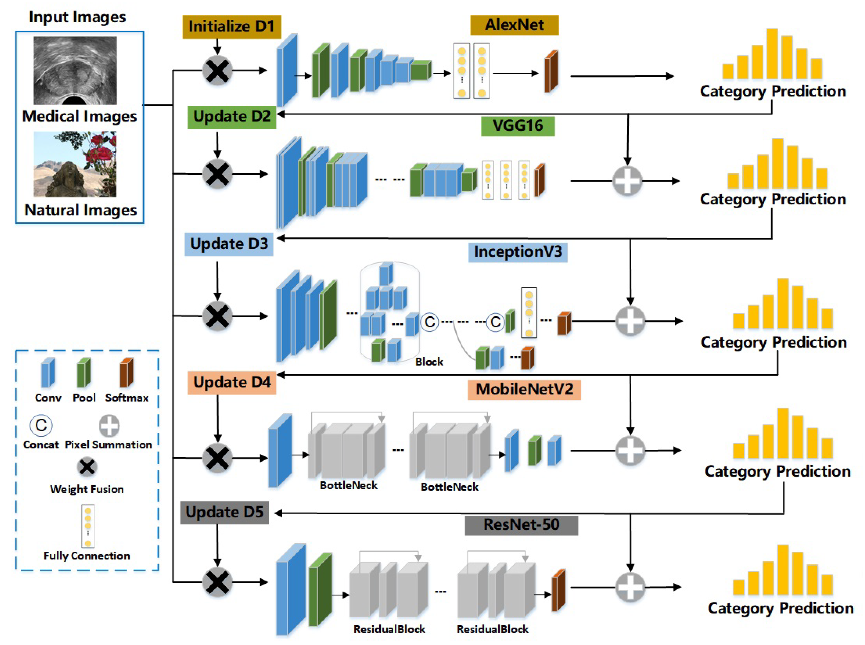
Based on the basic concept of ensemble learning, we try to aggregate multiple CNNs into a strong image classification model [1,47,48]. However, unlike traditional ensemble learning methods or Adaboost CNNs [38], which consist of the same type of sub-networks that are indiscriminately trained and tested, our HCNN consists of several different types of CNNs as the sub-networks, and these sub-networks are trained progressively in order. In this paper, we choose Alexnet [10], VGG16 [11], Inception V3 [49], Mobilenet V2 [50], and Resnet-50 [12] as the basic sub-networks (see Figure 1). In addition, there are no limits on the number of sub-networks and their types. At the training stage, images are assigned weights to express the difficulties encountered by models in accurately classifying them. If an image can not be accurately classified by a sub-network, its weight will be increased. Images with updated weights are then input into the next sub-network for extracting more abstract and effective visual features. In this section, we will elaborate on HCNNs in more detail.

Figure 1.
An overview of HCNNs. In this paper, the HCNN consists of five sub-networks, i.e., Alexnet, VGG16, Inception V3, Mobilenet, and Resnet-50. Each image sample has its weight for the specific sub-networks. represent the image weights for the sub-networks, respectively. Each sub-network combines the results of the previous sub-networks to make decisions.
Assume that HCNNs have M sub-networks, and they are trained one by one. Let be the weight of the i-th image for the m-th sub-network, and . Here, , , while n is the number of all images in the training dataset.
First of all, the weights of all images need to be initialized. We therefore input all these training images with their initial weights into the first sub-network (Alexnet, ) for model training.
where . The first sub-network is then trained through multiple iterations. The gradient descent is used to update its parameters in each iteration. Finally, the trained sub-network can give the predictions:
where represents the m-th sub-network, and is the predicted label of the i-th sample by the m-th sub-network . Next, we select the samples that meet the condition of , where is the ground truth of the category label of the i-th sample. We further use the following equation to calculate the weighted error rate of the m-th sub-network on all selected samples in the training set:
where is the weight of the -th selected samples for , and is the number of selected samples. Subsequently, is used to obtain the weight coefficient of , which denotes the importance coefficient of in HCNNs:
As Equation (4) shows, is inversely proportional to , i.e., with a smaller error rate , the corresponding sub-network will have larger values of the importance coefficient throughout the whole model. Furthermore, is used to update the weights of the samples to train the next sub-network.
For the images that meet the condition , we have
Otherwise,
Then,
Therefore, if the predicted results exhibit a high degree of agreement with the true labels of the images, then the weights of the images for the next sub-network decrease; otherwise, their weights increase. We then use the image samples with their updated weights to train the next sub-network for multiple iterations.
For a dataset containing a small number of samples, the initial and updated weights of the samples are applicable to training of HCNNs. However, if the dataset consists of a large number of samples, there is a risk of gradient explosion occurring during model training due to the loss values being too small (possibly even approaching zero); this means that the network parameters cannot be updated normally. To solve this problem, we use the weights of samples to obtain the category weights using Equation (8):
where represents the weight of the j-th category for the -th sub-network, and is the weight of the -th sample belonging to the j-th category, which has samples. We then use as the weights of the samples belonging to the j-th category (Equation (9)).
Therefore, before training each sub-network, we need to update the weights of all samples according to the weights of their corresponding categories. The sub-network will then pay more attention to the samples with larger weights.
HCNN is a scalable model, and its architecture is illustrated in Figure 1. In addition, HCNN enhances the correlation between different sub-networks by transmitting the feature vectors and the sample weights in the previous sub-network to the next sub-network.
3.2. Multi-Class Joint Loss in HCNNs
During model training, we constantly updated the weights of the image categories and the images to express the difficulties encountered by the model. We then needed to design the loss function, which can guide the model to extract the specific visual features from different images. In addition, this loss function should attempt to make the difference in the visual features within the same category as small as possible, while the difference in the visual features in different categories should be as large as possible.
Cross-entropy loss with category weights. The cross-entropy function is a classic and commonly used loss function. In this paper, to enable the HCNN to select its corresponding sub-networks and therefore extract the visual features in different levels, a category weight is assigned to each image category; subsequently, the new cross-entropy loss with category weights can be expressed by the following equation:
Here, is the cross-entropy loss with category weights for the -th sub-network, and is the traditional cross-entropy loss.
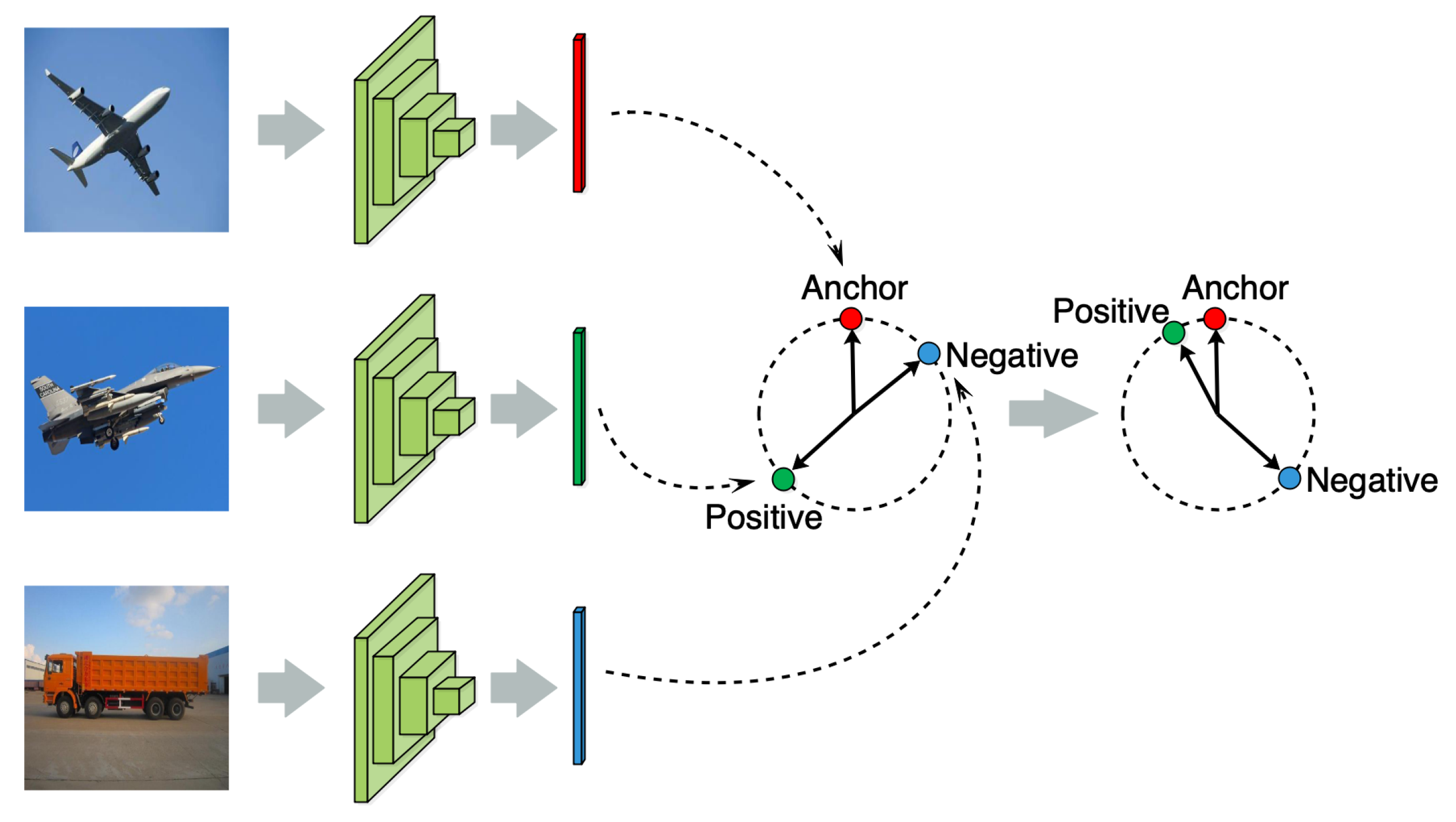
Weighted triplet loss. For image classification, the problem may arise that there may be less similarity between images within the same category, while there is more similarity between images in different categories; as a result, it is difficult to effectively improve the image classification performance. The triplet loss can guide models to learn the visual features to further cluster the samples within the same category and separate the samples of different categories. Therefore, we use a weighted triplet loss in each sub-network. This guides HCNNs to extract more discriminative visual features between the samples of different categories, as shown in Figure 2.

Figure 2.
An illustration of the influence of triplet loss on visual feature learning.
Assume that we have a series of image samples , and are their true labels. We then define an anchor image , a positive image sample , and a negative image sample . More specifically, is an image in one category, is another image in the same category with , and is an image in another category that differs from the category of . During model training, we can obtain a triplet set consisting of , , and in each batch, and then randomly select the corresponding samples to form a triple as the input of each sub-network. We can then obtain the triplet loss for the m-th sub-network:
Here, , , and represent the visual features extracted by the m-th sub-network from the images of , respectively, while is the Euclidean distance. Moreover, is a threshold parameter used to distinguish between the positive and negative samples of the anchor samples. is a parameter that is close to 0 without being equal to 0. Triplet loss is used to reduce the distance between the features of and and expand the distance between the features of and , as shown in Figure 2. Then, triplet loss can be used to solve the following three situations in HCNNs.
Case I: If , then . This situation shows that the current sub-network can accurately classify these three image samples; thus, there is no need to pay more attention to them in the subsequent sub-networks.
Case II: . This situation shows that high similarity exists among these three image samples, and the current sub-network finds it difficult to distinguish them. This triple S then needs to pass through the subsequent sub-networks with more complex network structures.
Case III: . This situation shows that the current sub-network cannot distinguish these image samples, and that their more abstract features need to be extracted by the subsequent sub-networks.
Weighted multi-class joint loss function. HCNNs can progressively classify images and achieve visual feature learning at different levels. In addition, in each batch during model training, a weighted multi-class joint loss function is designed by combining cross-entropy loss with category weights and weighted triplet loss.
Here, is the weighted multi-class joint loss for the m-th sub-network. is a hyperparameter; in this paper, .
3.3. Model Testing
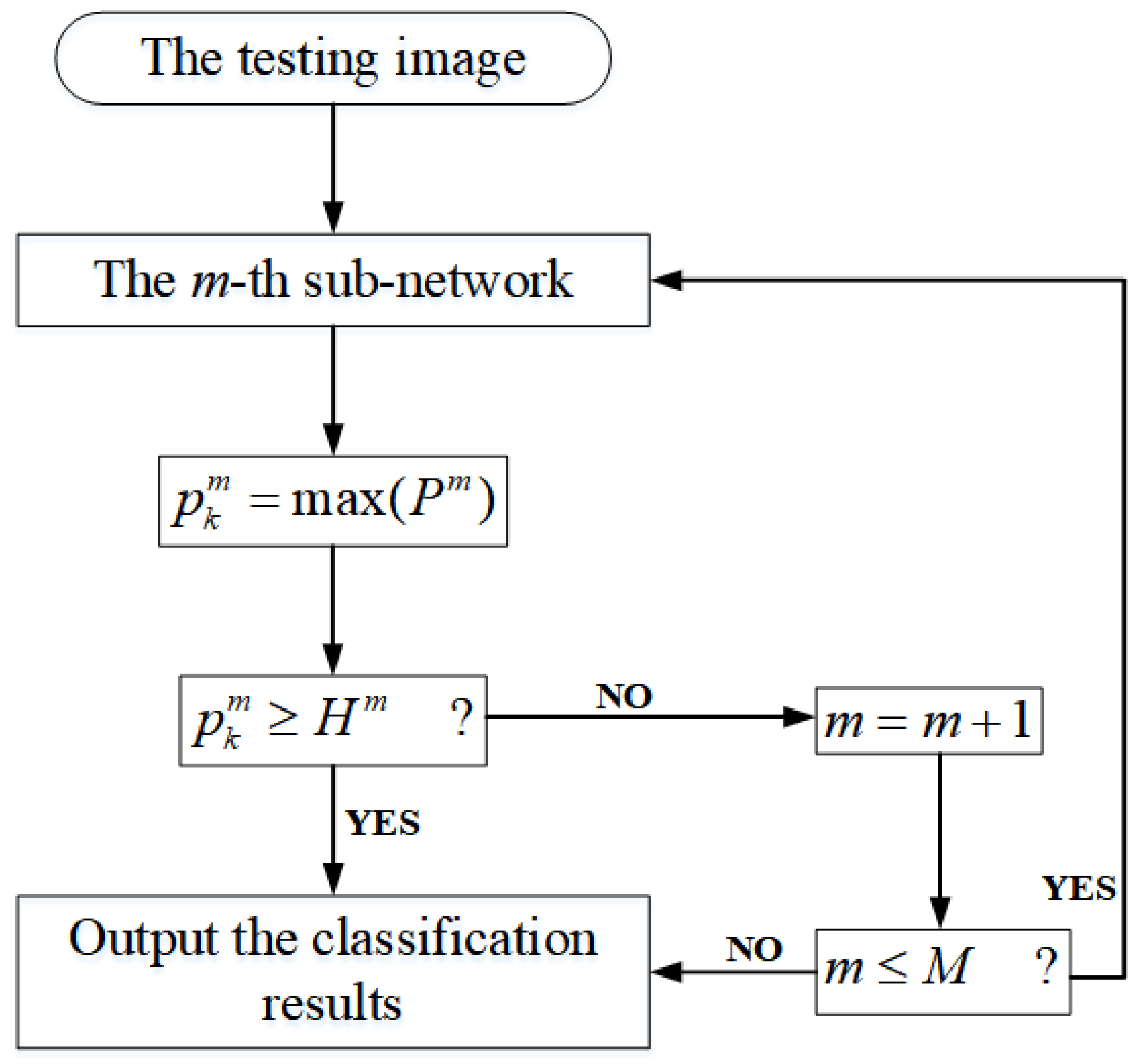
To test the proposed model, we need to provide a threshold for each sub-network so as to make the model output the final classification results. When image classification confidence in the m-th sub-network is higher than , this prediction is reliable; otherwise, the credibility of the image classification results is lower. Generally speaking, the values of can be set larger, which ensures that the difficult-to-identify images can pass through the subsequent sub-networks with more complex network structures. Figure 3 shows the simple process of image classification of HCNNs.
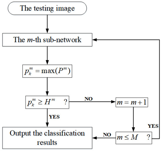
Figure 3.
Progressive image classification by HCNNs in the test stage.
In more detail, the testing process of HCNNs with M sub-networks can be described as follows.
- Step 1: The test image is input into the m-th sub-network for visual feature learning ( for the first sub-network). The model then outputs the probability distribution of the image classification results , where is the number of image categories.
- Step 2: A comparison is drawn between the maximum classification probability and .
- Step 3: If or , then the model outputs the classification results corresponding to ; otherwise, , and return to Step 1.
4. Experimental Results and Analysis
To verify the effectiveness and superiority of the proposed HCNN, we implement our model on two challenging image classification datasets (our ultrasonic prostate image dataset and the chimpanzee dataset [25]) and two commonly used image classification datasets (CIFAR-10 and CIFAR-100 [24]). Furthermore, we also utilize several related existing DNN models for comparative experimental analysis. In addition, we conduct ablation experiments to verify the influences of different sub-networks.
4.1. Image Classification Datasets
- (1)
- Ultrasonic image dataset of prostate
There have been related works on medical image datasets [51,52,53,54], while there are few works for prostate cancer screening. The traditional method of prostate cancer screening usually uses prostate biopsy puncture to obtain the pathological results, which causes great pain for patients. Therefore, we have collected ultrasonic images of prostate, and attempted to design CNN-based models for prostate cancer screening. Our ultrasonic image dataset of prostate has 932 images, which were selected from a number of ultrasonic images according to doctors’ experience. We divided these ultrasound images into two categories: the ultrasound images of patients with prostate cancer and those of patients without prostate cancer.
- (2)
- The chimpanzee facial image dataset
The chimpanzee dataset is provided by Loos et al. in [25]. The chimpanzee facial images were captured at Zoo Leipzig in Germany and Taï National Park in Africa. There are large numbers of images with weak or highlight illumination, incomplete facial contours, partial occlusion by branches or leaves, and inconsistent image sizes. This image dataset is therefore very challenging for the image classification task. Table 1 presents the details of the chimpanzee facial images used in this paper. We selected at least five images for each chimpanzee individual from the entire dataset as our test images.

Table 1.
Datasets summary.
- (3)
- CIFAR-10 and CIFAR-100
CIFAR-10 and CIFAR-100 contain 60,000 images each, where each color image has 32 × 32 pixels. CIFAR-10 comprises 10 categories (aircraft, car, bird, cat, deer, dog, frog, horse, boat, truck). As in previous works, we also use 50,000 images for model training and 10,000 images for testing, and there are no duplicate image samples. In addition, we select 20% of the training images as the validation image dataset. CIFAR-100 consists of the image samples of 100 categories, and we also divide these into 50,000 training images and 10,000 testing images. The training, validation, and testing image sets are allocated according to a ratio of 9:1:2 in the whole CIFAR-100 image dataset (as shown in Table 1).
4.2. Experimental Setup
The proposed HCNN is an image classification model based on ensemble learning. In this paper, we choose Alexnet [10], VGG16 [11], Inception V3 (I_V3) [49], Mobilenet V2 (M_V2) [50], and Resnet-50 [12] as the basic sub-networks. Of course, in specific tasks, the types of sub-networks can be changed, and we also can add or subtract sub-networks. We further implement several existing deep learning models and ensemble learning models as the comparison models. The experimental results of our model are compared with these basic sub-networks by using the same parameters. We further make comparisons of our model with Adaboost-CNN [38] on CIFAR-10, and with Wide-ResNet 40-2 [55], Wide-ResNet 40-2+CutMix [56], DenseNet-100 [57], and DenseNet-100+CutMix [56] on CIFAR-100. In addition, to verify the gradual improvements achieved by HCNNs, we draw comparisons of HCNNs with the single sub-networks and their different combinations.
For each image dataset, we set the batch size to 10, and the initial learning rate is 0.0001. We set in Equation (12) to 0.5. The dimensions of , and in triplet loss are set to 256 uniformly. All models used in this paper were implemented on three TITAN Xp GPUs.
4.3. Experimental Results
- (1)
- Experimental results on the ultrasonic image dataset
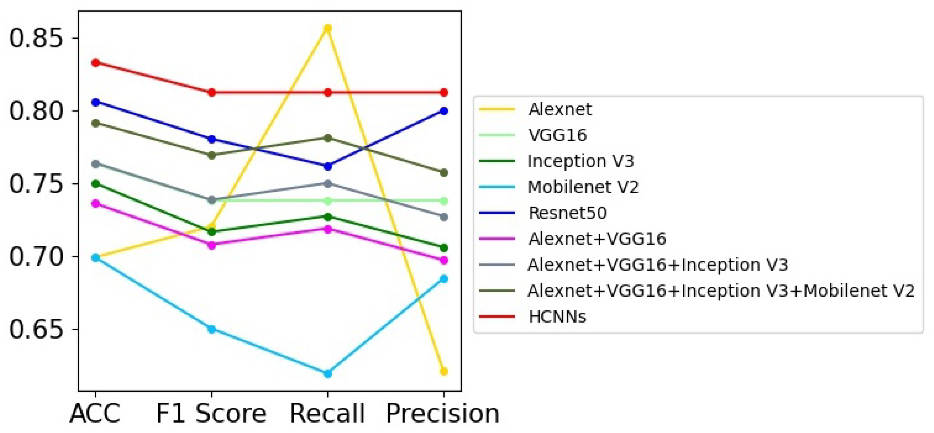
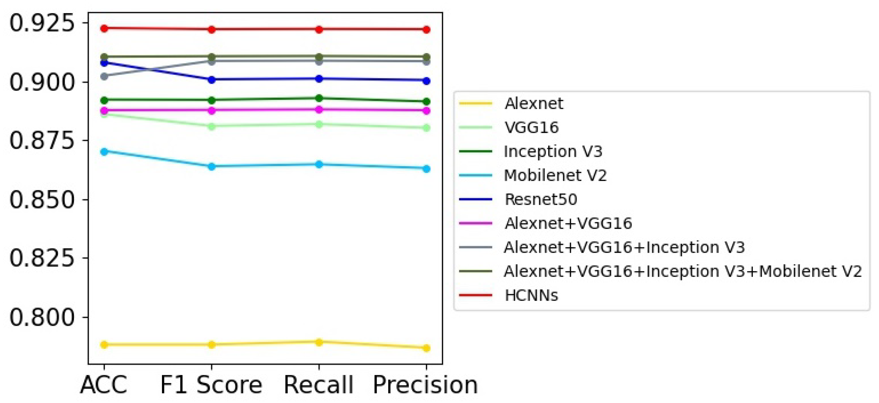
Prostate cancer screening based on ultrasound images is mainly used to distinguish whether the patients have prostate cancer or not according to their prostate ultrasound images. It can be regarded as a binary image classification problem. However, the prostate ultrasound images are fairly complex, and the lesions are not obvious, so it is difficult for professional doctors to diagnose prostate diseases only using ultrasound images. Therefore, there are challenges for the automatic screening of prostate cancer utilizing computer vision technologies from ultrasound images. In this paper, we try to use several DNN models to perform the binary image classification task, and the experimental results are shown in Table 2. We can obtain the following points from the experimental results. First, all the models used in this paper fail to achieve perfect image classification performance, and the highest recognition accuracy is lower than 85%, which shows that there is difficulty in recognizing prostate cancer. Second, Resnet50 achieves better performance among the single deep network models. It has 4.31% higher accuracy than VGG16, and 5.65% higher than Inception V3. Third, the models combing multiple networks have increasing accuracies; for example, “Alexnet+VGG16+Inception V3+Mobilenet V2” has 2.83% higher accuracy than VGG16. Among these methods, the HCNN with five deep networks achieves the best performance, and it has 2.68% higher accuracy than Resnet50. Figure 4 shows the graph of Table 2; we can see that HCNN achieves obvious advantages over other models in most evaluation indicators. In addition, the performance would be further improved with the improvement or addition of the sub-networks.
Table 2.
The ablation analysis on the ultrasonic image dataset.
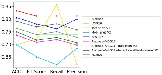
Figure 4.
The curve graph of Table 2.
- (2)
- Experimental results on the chimpanzee facial image dataset
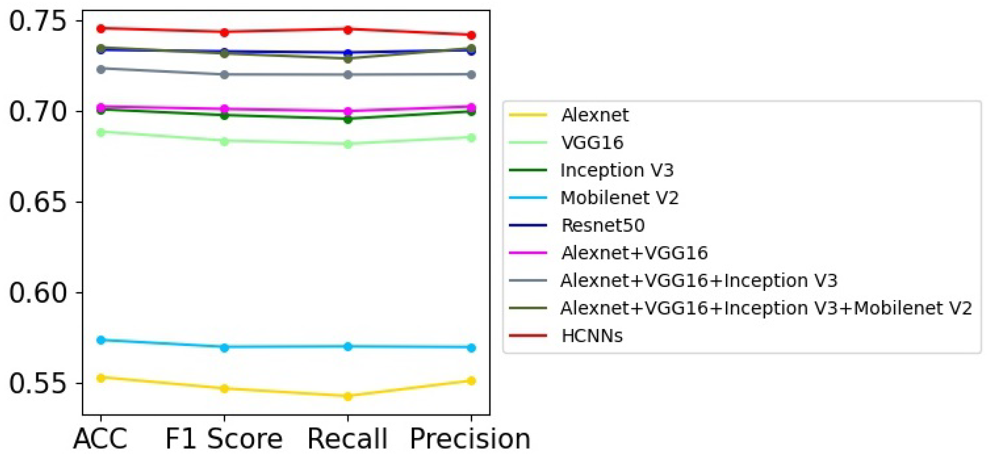
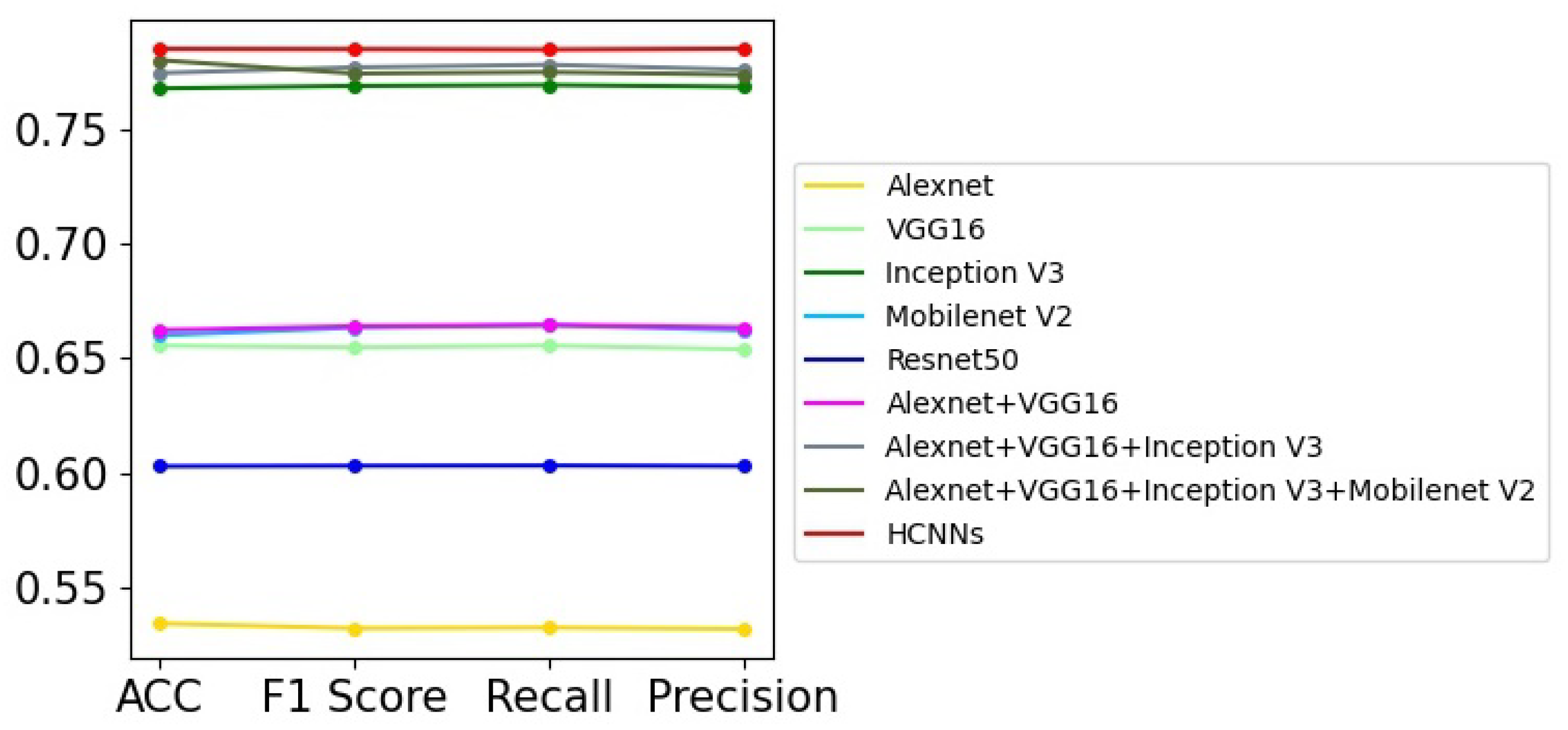
There are a large number of challenging chimpanzee facial images in the chimpanzee facial image dataset [25]; it is therefore difficult for models to achieve good image classification performance. In this paper, we implement nine different models on this dataset; the experimental results are shown in Table 3, where we can see that these models, which perform well on some public image classification databases, do not perform well on this chimpanzee facial image dataset. The model with the single network that works best is Resnet50, with 0.7336% accuracy, while the HCNN achieves the highest image classification accuracy of 74.55%. Figure 5 shows the curves of these models’ performance in related evaluation indicators, and it can be seen that the HCNN has general advantages over models with single neural networks and other models with multiple sub-networks in terms of F1 score, recall, and precision, which clearly demonstrates its effectiveness and superiority.
Table 3.
The ablation analysis on the chimpanzee facial image dataset.
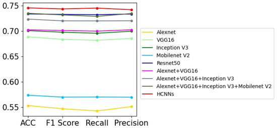
Figure 5.
The curve graph of Table 3.
- (3)
- Experimental results on CIFAR-10
Table 4 presents the experimental results of nine different models on CIFAR-10; these models include the sub-networks in HCNNs and their different combinations. For each model, we carried out 20 epochs of model training. From the results shown in Table 4, we can see that Resnet50 [12] achieves the best performance among all models with a single network. Furthermore, the ensemble learning models with different sub-networks achieve general improvements over the corresponding single-network models, which proves the effectiveness of ensemble learning models. Therefore, HCNN achieves the final best performance, with test accuracy of 92.26% on CIFAR-10, and 1.46–13.45% higher classification accuracy than the other five basic sub-networks. In addition, HCNN also has advantages in terms of F1 score, recall, and precision. In Figure 6, the performance difference among these models can be illustrated more clearly. Although these models achieved better results on CIFAR-10 than on the ultrasonic image dataset and chimpanzee facial image dataset, the overall trends of the models’ performance are similar. The reasons may be that the weights of the training samples for each sub-network in HCNNs are updated according to the classification results of the previous sub-network. In this way, different sub-networks can learn the specific features from the images, and present various degrees of difficulty to the various models that attempt to accurately classify them. Therefore, HCNNs can progressively learn the visual features at different levels and gradually improve the image classification performance.
Table 4.
The ablation analysis on the CIFAR-10 dataset.

Figure 6.
The curve graph of Table 4.
AdaBoost-CNN [38], proposed by Taherkhani et al., is also an ensemble learning model based on DNNs. Its test accuracy on CIFAR-10 reaches 81.40%, as shown in Table 5. By contrast, our HCNN has 10.86% higher accuracy. Adaboost-CNN creates a classification model with better performance by combining several simple convolutional sub-networks. However, multiple sub-networks in Adaboost-CNN use the same network structure, and each sub-network is only fine-tuned on the parameters of its previous sub-network. Therefore, it is difficult for the model to learn the specific abstract visual features from the images; this may be the reason for the limited performance of Adaboost-CNN.
Table 5.
The experimental analysis of Adaboost-CNN and HCNN on the CIFAR-10 dataset.
- (4)
- Experimental results on CIFAR-100
CIFAR-100 contains more image categories than CIFAR-10 and is less able to achieve higher image classification accuracy for classification models. Fourteen different models are implemented in CIFAR-100, and the experimental results are shown in Table 6 and Table 7 and Figure 7. From the test results shown in Table 6, it can be seen that the models combining different sub-networks achieve better performance than models with a single neural network, which is similar to Table 4. The HCNN, with a test accuracy of 78.47%, achieves accuracy that is 9.46% higher than that of Mobilenet V2 and 1.72% higher than that of Inception V3, which represents the best performance among the single neural network models.
Table 6.
The ablation analysis on the CIFAR-100 dataset.
Table 7.
The experimental results of Adaboost-CNN and HCNN on the CIFAR-100 dataset.

Figure 7.
The curve graph of Table 6.
Moreover, as shown in Table 7, HCNN achieves similar performance to DenseNet-100+CutMix [56], but is better than other existing network models with complex network structures. During the image classification process, each image (regardless of whether it is easy or difficult for the model to accurately classify) needs to go through these complex network models to extract visual features. In HCNNs, however, different images will pass through different levels of sub-networks, and the model will learn specific visual features from images at different levels. Therefore, HCNN achieves better effectiveness and efficiency for image classification.
5. Conclusions
At present, all the image classification models treat the images equally. However, there are meaningful differences between images, so different images should be treated differently by various models, which would comply with the basic mechanism of human cognition. Therefore, we propose HCNNs, which classify different images by different numbers of sub-networks. In HCNNs, the easy-to-identify images are recognized by simple sub-networks and output the results directly, while images that are more difficult to identify may need to go through multiple complex sub-networks to extract their more abstract visual features. Through this image classification mechanism, HCNNs achieve better image classification performance compared with existing single-network models and Adaboost CNN with its multiple simple sub-networks. In addition, the HCNN has better scalability and variability; that is, the number of sub-networks can be increased or decreased, and the types of sub-networks can be changed according to the specific visual tasks involved. Therefore, in the future, more detailed models similar to HCNNs may be constructed based on the complexity of the image classification task, which would gradually become closer to the basic mechanism of human cognition, and the models will have higher recognition accuracy and efficiency.
Author Contributions
C.L. designed the research and wrote the manuscript. F.M. contributed to the improvement of the ideas and to the revision of the manuscript. G.G. carried out the data collection and research experiments. All authors have read and agreed to the published version of the manuscript.
Funding
This research was funded by National Natural Science Foundation of China under grant agreements Nos. 61973250, 61973249, 62073218, 61802335, 61902313, 61902296, 61971349; Shaanxi Province Science Fund for Distinguished Young Scholars: 2018JC-016; Shaanxi Provincial Department of Education serves local scientific research: 19JC038; and the Key Research and Development Program of Shaanxi: 2021GY-077, 2020ZDLGY04-07, 2021ZDLGY02-06, 2019GY-012.
Informed Consent Statement
Informed consent was obtained from all subjects involved in the study.
Data Availability Statement
The images in Ultrasonic image dataset of prostate are collected from Department of Ultrasound, Ruijin Hospital, Shanghai Jiao Tong University School of Medicine, Shanghai, China, and these used images have no personal information of patients. Chimpanzee facial image dataset, CIFAR-10 and CIFAR-100 are public image datasets.
Conflicts of Interest
All the authors declare that we have no known competing financial interests or personal relationships that could have appeared to influence the work reported in this paper.
References
- Nie, L.; Zhang, L.; Meng, L.; Song, X.; Chang, X.; Li, X. Modeling disease progression via multisource multitask learners: A case study with Alzheimer’s disease. IEEE Trans. Neural Netw. Learn. Syst. 2016, 28, 1508–1519. [Google Scholar] [CrossRef]
- Luo, M.; Chang, X.; Nie, L.; Yang, Y.; Hauptmann, A.G.; Zheng, Q. An adaptive semisupervised feature analysis for video semantic recognition. IEEE Trans. Cybern. 2017, 48, 648–660. [Google Scholar] [CrossRef]
- Wang, S.; Chang, X.; Li, X.; Long, G.; Yao, L.; Sheng, Q.Z. Diagnosis code assignment using sparsity-based disease correlation embedding. IEEE Trans. Knowl. Data Eng. 2016, 28, 3191–3202. [Google Scholar] [CrossRef] [Green Version]
- Qi, L.; Tang, W.; Zhou, L.; Huang, Y.; Zhao, S.; Liu, L.; Li, M.; Zhang, L.; Feng, S.; Hou, D.; et al. Long-term follow-up of persistent pulmonary pure ground-glass nodules with deep learning–assisted nodule segmentation. Eur. Radiol. 2020, 30, 744–755. [Google Scholar] [CrossRef] [PubMed]
- Munir, K.; Elahi, H.; Ayub, A.; Frezza, F.; Rizzi, A. Cancer Diagnosis Using Deep Learning: A Bibliographic Review. Cancers 2019, 11, 1235. [Google Scholar] [CrossRef] [PubMed] [Green Version]
- Liu, B.; Chi, W.; Li, X.; Li, P.; Liang, W.; Liu, H.; Wang, W.; He, J. Evolving the pulmonary nodules diagnosis from classical approaches to deep learning-aided decision support: Three decades’ development course and future prospect. J. Cancer Res. Clin. Oncol. Vol. 2020, 146, 153–185. [Google Scholar] [CrossRef] [PubMed] [Green Version]
- Cheng, Z.; Chang, X.; Zhu, L.; Kanjirathinkal, R.C.; Kankanhalli, M. MMALFM: Explainable recommendation by leveraging reviews and images. ACM Trans. Inf. Syst. (TOIS) 2019, 37, 1–28. [Google Scholar] [CrossRef]
- Li, Z.; Yao, L.; Chang, X.; Zhan, K.; Sun, J.; Zhang, H. Zero-shot event detection via event-adaptive concept relevance mining. Pattern Recognit. 2019, 88, 595–603. [Google Scholar] [CrossRef]
- Yu, E.; Sun, J.; Li, J.; Chang, X.; Han, X.H.; Hauptmann, A.G. Adaptive semi-supervised feature selection for cross-modal retrieval. IEEE Trans. Multimed. 2018, 21, 1276–1288. [Google Scholar] [CrossRef]
- Krizhevsky, A.; Sutskever, L.; Hinton, G.E. Imagenet classification withdeep convolutional neural networks. Adv. Neural Inf. Process. Syst. 2012, 25, 1097–1105. [Google Scholar]
- Simonyan, K.; Zisserman, A. Very deep convolutional networks for large-scale image recognition. arXiv 2014, arXiv:1409.1556. [Google Scholar]
- He, K.; Zhang, X.; Ren, S.; Sun, J. Deep residual learning for image recog-nition. In Proceedings of the IEEE Conference on Computer Vision and Pattern Recognition, Las Vegas, NV, USA, 27–30 June 2016; pp. 770–778. [Google Scholar]
- Forres, I.; Matt, M.; Serge, K.; Ross, G.; Trevor, K.; Kurt, K. Densenet: Im-plementing efficient convnet descriptor pyramids. arXiv 2014, arXiv:1404.1869. [Google Scholar]
- Qiang, L.; Xuyu, X.; Jiaohua, Q.; Yun, T.; Yuanjing, T.J.L. Cover-less steganography based on image retrieval of densenet features and dwtsequence mapping. Knowl.-Based Syst. 2020, 192, 105375. [Google Scholar]
- Zhang, D.; Yao, L.; Chen, K.; Wang, S.; Chang, X.; Liu, Y. Making sense of spatio-temporal preserving representations for EEG-based human intention recognition. IEEE Trans. Cybern. 2019, 50, 3033–3044. [Google Scholar] [CrossRef] [PubMed]
- Nie, L.; Zhang, L.; Yan, Y.; Chang, X.; Liu, M.; Shaoling, L. Multiview physician-specific attributes fusion for health seeking. IEEE Trans. Cybern. 2016, 47, 3680–3691. [Google Scholar] [CrossRef] [Green Version]
- Ren, P.; Xiao, Y.; Chang, X.; Huang, P.Y.; Li, Z.; Chen, X.; Wang, X. A comprehensive survey of neural architecture search: Challenges and solutions. ACM Comput. Surv. (CSUR) 2021, 54, 1–34. [Google Scholar] [CrossRef]
- Li, Z.; Nie, F.; Chang, X.; Yang, Y. Beyond trace ratio: Weighted harmonic mean of trace ratios for multiclass discriminant analysis. IEEE Trans. Knowl. Data Eng. 2017, 29, 2100–2110. [Google Scholar] [CrossRef]
- Yuan, D.; Chang, X.; Huang, P.Y.; Liu, Q.; He, Z. Self-supervised deep correlation tracking. IEEE Trans. Image Process. 2020, 30, 976–985. [Google Scholar] [CrossRef]
- Ma, Z.; Chang, X.; Yang, Y.; Sebe, N.; Hauptmann, A.G. The many shades of negativity. IEEE Trans. Multimed. 2017, 19, 1558–1568. [Google Scholar] [CrossRef]
- Li, Z.; Nie, F.; Chang, X.; Yang, Y.; Zhang, C.; Sebe, N. Dynamic affinity graph construction for spectral clustering using multiple features. IEEE Trans. Neural Netw. Learn. Syst. 2018, 29, 6323–6332. [Google Scholar] [CrossRef] [PubMed]
- Yan, C.; Zheng, Q.; Chang, X.; Luo, M.; Yeh, C.H.; Hauptman, A.G. Semantics-preserving graph propagation for zero-shot object detection. IEEE Trans. Image Process. 2020, 29, 8163–8176. [Google Scholar] [CrossRef] [PubMed]
- Ren, P.; Xiao, Y.; Chang, X.; Huang, P.Y.; Li, Z.; Gupta, B.; Wang, X. A Survey of Deep Active Learning. ACM Comput. Surv. (CSUR) 2021, 54, 1–40. [Google Scholar] [CrossRef]
- Krizhevsky, A.; Hinton, G. Learning multiple layers of features fromtiny images. Tech Rep. 2009, 7, 1–60. [Google Scholar]
- Loos, A.; Ernst, A. An automated chimpanzee identification system using face detection and recognition. EURASIP J. Image Video Process. 2013, 2013, 49. [Google Scholar] [CrossRef]
- Khan, S.; Nazir, S.; Garcia-Magarino, I.; Hussain, A. Deep learning-base urban big data fusion in smart cities: Towards traffic monitoring and flow-preserving fusion. Comput. Electr. Eng. 2021, 89, 106906. [Google Scholar] [CrossRef]
- Orozco, M.C.E.; Rebong, C.B. Vehicular detection and classification forintelligent transportation system: A deep learning approach using faster490r-cnn model. Int. J. Simul. Syst. 2019, 180, 36551. [Google Scholar]
- Zhenghao, X.; Niu, Y.; Chen, J.; Kan, X.; Liu, H. Facial expression recognition of industrial internet of things by parallel neural networks combining texture features. IEEE Trans. Ind. Inform. 2020, 17, 2784–2793. [Google Scholar]
- Hossain, M.S.; Muhammad, G.; Amin, S.U. Improving consumer satisfac-tion in smart cities using edge computing and caching: A case study ofdate fruits classification. Future Gener. Comput. Syst. 2018, 88, 333–341. [Google Scholar] [CrossRef]
- Gören, S.; Óncevarlk, D.F.; Yldz, K.D.; Hakyemez, T.Z. On-street parking500spot detection for smart cities. In Proceedings of the IEEE International Smart CitiesConference (ISC2), Casablanca, Morocco, 14–17 October 2019; pp. 292–295. [Google Scholar]
- Yao, H.; Gao, P.; Wang, J.; Zhang, P.; Jiang, C.; Han, Z. Capsule networkassisted iot traffic classification mechanism for smart cities. IEEE Internet Things J. 2019, 6, 7515–7525. [Google Scholar] [CrossRef]
- Hassan, A.; Liu, F.; Wang, F.; Wang, Y. Secure image classification withdeep neural networks for iot applications. J. Ambient Intell. Humaniz. Comput. 2020, 12, 8319–8337. [Google Scholar] [CrossRef]
- Vasan, D.; Alazab, M.; Wassan, S.; Naeem, H.; Safaei, B.; Zheng, Q. Imcfn:Image-based malware classification using fine-tuned convolutional neural network architecture. Comput. Netw. 2020, 171, 107138. [Google Scholar] [CrossRef]
- Ciregan, D.; Meier, U.; Schmidhuber, J. Multi-column deep neural networksfor image classification. In Proceedings of the IEEE Conference on Computer Vision and Pattern Recognition, Providence, RI, USA, 16–21 June 2012; pp. 3642–3649. [Google Scholar]
- Frazao, X.; Alexandre, L.A. Weighted convolutional neural network ensemble. In Iberoamerican Congress on Pattern Recognition; Springer: Cham, Switzerland, 2014; pp. 674–681. [Google Scholar]
- Tajbakhsh, N.; Gurudu, S.R.; Liang, J. Automatic polyp detection incolonoscopy videos using an ensemble of convolutional neural networks. In Proceedings of the 2015 IEEE 12th International Symposium on Biomedical Imaging (ISBI), Brooklyn, NY, USA, 16–19 April 2015; pp. 79–83. [Google Scholar]
- Ijjina, E.P.; Mohan, C.K. Hybrid deep neural network model for humanaction recognition. Appl. Soft Comput. 2016, 46, 936–952. [Google Scholar] [CrossRef]
- Taherkhani, A.; Cosma, G.; McGinnity, T.M. Adaboost-cnn: An adaptiveboosting algorithm for convolutional neural networks to classify multi-classimbalanced datasets using transfer learning. Neurocomputing 2020, 404, 351–366. [Google Scholar] [CrossRef]
- Movshovitz-Attias, Y.; Toshev, A.; Leung, T.K.; Ioffe, S.; Singh, S. No fussdistance metric learning using proxies. In Proceedings of the IEEE International Conferenceon Computer Vision, Venice, Italy, 22–29 October 2017; pp. 360–368. [Google Scholar]
- Liu, W.; Wen, Y.; Yu, Z.; Li, M.; Raj, B.; Song, L. Sphereface: Deep hy-persphere embedding for face recognition. In Proceedings of the IEEE Conference on Computer Vision and Pattern Recognition, Honolulu, HI, USA, 21–26 July 2017; pp. 212–220. [Google Scholar]
- Chen, W.; Chen, X.; Zhang, J.; Huang, K. Beyond triplet loss: A deepquadruplet network for person re-identification. In Proceedings of the IEEE Conference on Computer Vision and Pattern Recognition, Honolulu, HI, USA, 21–26 July 2017; pp. 403–412. [Google Scholar]
- Schroff, F.; Kalenichenko, D.; Philbin, J. Facenet: A unified embedding forface recognition and clustering. In Proceedings of the IEEE Conference on Computer Vision and Pattern Recognition, Boston, MA, USA, 7–12 June 2015; pp. 815–823. [Google Scholar]
- Wang, X.; Han, X.; Huang, W.; Dong, D.; Scott, M.R. Multi-similarity loss with general pair weighting for deep metric learning. In Proceedings of the IEEE Conference on Computer Vision and Pattern Recognition, Long Beach, CA, USA, 16–20 June 2019; pp. 5022–5030. [Google Scholar]
- Wen, Y.; Zhang, K.; Li, Z.; Qiao, Y. A discriminative feature learning approach for deep face recognition. In Proceedings of the European Conference on Computer Vision, Amsterdam, The Netherlands, 11–14 October 2016; Springer: Cham, Switzerland, 2016; pp. 499–515. [Google Scholar]
- Wang, J.; Zhou, F.; Wen, S.; Liu, X.; Lin, Y. Deep metric learning withangular loss. In Proceedings of the IEEE International Conference on Computer Vision, Venice, Italy, 22–29 October 2017; pp. 2593–2601. [Google Scholar]
- Jiang, L.; Meng, D.; Yu, S.-I.; Lan, Z.; Shan, S.; Hauptmann, A. Self-paced learning with diversity. Adv. Neural Inf. Process. Syst. 2014, 27, 2078–2086. [Google Scholar]
- Chang, X.; Yu, Y.L.; Yang, Y.; Xing, E.P. Semantic pooling for complex event analysis in untrimmed videos. IEEE Trans. Pattern Anal. Mach. Intell. 2017, 39, 1617–1632. [Google Scholar] [CrossRef]
- Yan, C.; Chang, X.; Li, Z.; Guan, W.; Ge, Z.; Zhu, L.; Zheng, Q. ZeroNAS: Differentiable Generative Adversarial Networks Search for Zero-Shot Learning. IEEE Trans. Pattern Anal. Mach. Intell. 2021. [Google Scholar] [CrossRef] [PubMed]
- Szegedy, C.; Vanhoucke, V.; Ioffe, S.; Shlens, J.; Wojna, Z. Rethinking theinception architecture for computer vision. In Proceedings of the IEEE Conference on Computer Vision and Pattern Recognition, Las Vegas, NV, USA, 27–30 June 2016; pp. 2818–2826. [Google Scholar]
- Sandler, M.; Howard, A.; Zhu, M.; Zhmoginov, A.; Chen, L.-C. Mobilenetv2:Inverted residuals and linear bottlenecks. In Proceedings of the IEEE conference on computer vision and pattern recognition, Salt Lake City, UT, USA, 18–22 June 2018; pp. 4510–4520. [Google Scholar]
- Munir, K.; Frezza, F.; Rizzi, A. Deep Learning for Brain Tumor Segmentation. In Deep Learning for Cancer Diagnosis; Springer: Singapore, 2020; pp. 189–201. [Google Scholar]
- Munir, K.; Elahi, H.; Farooq, M.U.; Ahmed, S.; Frezza, F.; Rizzi, A. Detection and screening of COVID-19 through chest computed tomography radiographs using deep neural networks. In Data Science for COVID-19; Academic Press: Cambridge, MA, USA, 2021; pp. 63–73. [Google Scholar]
- Munir, K.; Frezza, F.; Rizzi, A. Brain Tumor Segmentation Using 2D-UNET Convolutional Neural Network. In Deep Learning for Cancer Diagnosis; Springer: Singapore, 2020; pp. 239–248. [Google Scholar]
- Fakoor, R.; Ladhak, F.; Nazi, A.; Huber, M. Using deep learning to enhance cancer diagnosis and classification. In Proceedings of the 30th International Conference on Machine Learning (ICML 2013), Atlanta, GA, USA, 16–21 June 2013. [Google Scholar]
- Zagoruyko, S.; Komodakis, N. Wide residual networks. arXiv 2016, arXiv:1605.07146. [Google Scholar]
- Yun, S.; Han, D.; Oh, S.J.; Chun, S.; Choe, J.; Yoo, Y. Cutmix: Regulariza-tion strategy to train strong classifiers with localizable features. In Proceedings of the IEEE International Conference on Computer Vision, Seoul, Korea, 27–28 October 2019; pp. 6023–6032. [Google Scholar]
- Huang, G.; Liu, Z.; Maaten, L.V.D.; Weinberger, K.Q. Densely con-nected convolutional networks. In Proceedings of the IEEE Conference on Computer Vision and Pattern Recognition, Honolulu, HI, USA, 21–26 July 2017; pp. 4700–4708. [Google Scholar]
Publisher’s Note: MDPI stays neutral with regard to jurisdictional claims in published maps and institutional affiliations. |
© 2021 by the authors. Licensee MDPI, Basel, Switzerland. This article is an open access article distributed under the terms and conditions of the Creative Commons Attribution (CC BY) license (https://creativecommons.org/licenses/by/4.0/).