Article

Highly Robust Observer Sliding Mode Based Frequency Control for Multi Area Power Systems with Renewable Power Plants

1
Faculty of Electrical & Electronics Engineering, Ton Duc Thang University, Ho Chi Minh City 700000, Vietnam
2
Faculty of Electrical and Electronics Engineering, Ho Chi Minh City University of Technology and Education, Ho Chi Minh City 700000, Vietnam
3
Faculty of Industrial Engineering, Tien Giang University, Tien Giang Province 840000, Vietnam
*
Author to whom correspondence should be addressed.
Electronics 2021, 10(3), 274; https://doi.org/10.3390/electronics10030274
Submission received: 15 December 2020 / Revised: 13 January 2021 / Accepted: 21 January 2021 / Published: 24 January 2021

Abstract

:
This paper centers on the design of highly robust observer sliding mode (HROSM)-based load frequency and tie-power control to compensate for primary frequency control of multi-area interconnected power systems integrated with renewable power generation. At first, the power system with external disturbance is model in the state space form. Then the state observer is used to estimate the system states which are difficult or expensive to measure. Secondly, the sliding mode control (SMC) is designed with a new single phase sliding surface (SPSS). In addition, the whole system asymptotic stability is proven with Lyapunov stability theory based on the linear matrix inequality (LMI) technique. The new SPSS without reaching time guarantees rapid convergence of high transient frequency, tie-power change as well as reduces chattering without loss of accuracies. Therefore, the superiority of modern state-of-the-art SMC-based frequency controllers relies on good practical application. The experimental simulation results on large interconnected power systems show good performance and high robustness against external disturbances when compared with some modern state of art controllers in terms of overshoots and settling time.

1. Introduction

High level penetration of renewable generation systems into interconnected multi-area generation systems will make power sectors more economical and reliable to deliver power to end users. Since each area consists of increase numbers of generating sets, renewable power sets can be used as reservation for peak load demand. However, external disturbances such as intermittent generation associated with renewable sources and continuous load demand on one area can cause a high spike of frequency and tie-power flow in the multi-area [1]. Thus, frequency spike can damage power system equipment; can cause wear and tear of steam actuator valve, affects primary frequency control, etc. To solve this issue, load frequency control (LFC) is applied. LFC is one vital aspect of automatic generation control. Its duty is to compensate for primary control to ensure frequency and tie line flow at scheduled value [1]. Its design application in power systems follows two approaches, i.e., centralized and decentralized. The decentralized approach is commonly used since each local area is controlled on its own without interfering with neighboring areas. Furthermore, different techniques have been designed for LFC studies in various power systems. In the literature, early existing LFC methods were proportional-integral (PI) and proportional-integral-derivative (PID). These traditional schemes benefit in simple structures and performed well under parameters’ nominal operating points. However, they are degraded at variable points [2,3,4]. The degradation of PI and PID were solved with the development of intelligent control such as artificial neural network (ANN) and fuzzy logic given in [5,6,7,8]. Moreover, with the use of fuzzy logic, determining the accurate fuzzy set for tuning traditional control method is challenging. Optimal control techniques were applied with fuzzy logic to improve fuzzy set decision [9]. So far, both PI and intelligent control were combined to improve traditional LFC method [10,11,12,13,14,15]. Meanwhile, PI tuning has further improved with new algorithms given in [16,17,18]. Nevertheless, the major problem with interconnected power systems integrated with renewable power sets is that they result in a higher increase of the system order, the number of tuning control parameters, uncertainties in the system states and large external disturbances. When the power system is modeled, the external disturbance most especially cannot be avoided. Therefore, the requirement of the LFC must be robust against external disturbance in reality. Thus, sliding mode control (SMC) is used nowadays due to it robust against disturbance [19]. However, SMC based LFC is not new to control engineers. Various SMC-based LFC for power systems are briefly discussed. SMC was designed to control frequency, tie-power and area control errors for three area power system consisting of non-reheat, reheat and hydro-plant distributed in the areas [19]. Discrete-time SMC based LFC was constructed for controlling areas in power system with full state feedback [20]. A nonlinear SMC was proposed for mismatch power system with wind farms [21]. Furthermore, optimal LFC based SMC was designed for nonlinear power system [22]. Adaptive SMC based LFC for power systems are discussed in [23,24,25,26]. However, the SMC controllers discussed in the literature were designed with all power system states assumed to be measured. In practical power system, it is difficult to measure all system states [27]. To solve this problem, the SMC based observer technique is employed [28,29]. It estimates system states and filters higher frequency harmonics [30]. In addition, it provides cost effective design of LFC for power systems. SMC combined with an observer has been applied for LFC studies in power systems [31,32]. A robust higher observer SMC via nonlinear super twisting LFC was recently designed for multi-area power system with good performance and robustness of SMC which lies on the control switching law and sliding surface [31]. The switching laws ensure all system states deviations are driven to the sliding surface and remain therein. In studies, the robustness of an integral sliding surface combined with an observer was designed for the LFC of a power system which guarantees frequency deviation in the nominal value. However, these above SMCs combined with observer need time for the trajectories to reach the sliding surface, which may decrease the system performance [33]. In addition, a more robust controller without reaching time ensures system state trajectories starts from its surface at the initial time moment [33]. Therefore, the single phase sliding surface (SPSS) choice emerges to design sliding mode control. Thus, this motivates my interest to design an SMC via SPSS based on an observer for LFCs of a large power network. The novelties of this article are stated below:
The new SMC via SPSS does not need reaching time as compared to [31,32] which can guarantee better system performance.
The new SPSS and controller are designed to depend only on the observer which is useful for real power application where the system states variables are difficult or expensive to measure.
The whole system stabilization is theoretically proven using Lyapunov stability theory based new linear matrix inequality (LMI) technique.
Experimental simulation results depict the better performance in terms settling time and overshoot in comparison with recently results.

2. State Space Power System Model

In this part, we model the considered large interconnected power system and also the wind farms. Before proceeding, we briefly describe the power system which consists of three area interconnected electricity systems with non-reheat turbines shown in Figure 1. Areas 1 and 3 are integrated with wind power. Each block represents power generation components with their dynamics and subsystem parameters.
To derive the system states model, we begin from Area 1 to Area 3 in the following equation.
The frequency deviation of Areas 1, 2 and 3 is
Δ f ˙ 1 ( t ) = 1 T p 1 Δ f 1 ( t ) + K p 1 T p 1 Δ P m 1 ( t ) K p 1 T p 1 Δ P t i e 1 ( t ) a 31 K p 1 T p 1 Δ P t i e 3 ( t ) K p 1 T p 1 Δ P d 1 K p 1 T p 1 Δ P W 1
Δ f ˙ 2 ( t ) = 1 T p 2 Δ f 2 ( t ) + K p 2 T p 2 Δ P m 2 ( t ) a 12 K p 2 T p 2 Δ P t i e 1 ( t ) K p 2 T p 2 Δ P t i e 2 ( t ) K p 2 T p 2 Δ P d 2
Δ f ˙ 3 ( t ) = 1 T p 3 Δ f 3 ( t ) + K p 3 T p 3 Δ P m 3 ( t ) a 23 K p 3 T p 3 Δ P t i e 2 ( t ) K p 3 T p 3 Δ P t i e 3 ( t ) K p 3 T p 3 Δ P d 3 K p 3 T p 3 Δ P W 3
The mechanics power deviation of the 3-area power system are
Δ P ˙ m 1 ( t ) = 1 T t 1 Δ P m 1 ( t ) + 1 T t 1 Δ P v 1 ( t )
Δ P ˙ m 2 ( t ) = 1 T t 2 Δ P m 2 ( t ) + 1 T t 2 Δ P v 2 ( t )
Δ P ˙ m 3 ( t ) = 1 T t 3 Δ P m 3 ( t ) + 1 T t 3 Δ P v 3 ( t )
The valve position deviation of the 3-area power system are given as
Δ P ˙ v 1 ( t ) = 1 R 1 T g 1 Δ f 1 ( t ) 1 T g 1 Δ P v 1 ( t ) + 1 T g 1 u 1
Δ P ˙ v 2 ( t ) = 1 R 2 T g 2 Δ f 2 ( t ) 1 T g 2 Δ P v 2 ( t ) + 1 T g 2 u 2
Δ P ˙ v 3 ( t ) = 1 R 3 T g 3 Δ f 3 ( t ) 1 T g 3 Δ P v 3 ( t ) + 1 T g 3 u 3
The area control error of Areas 1, 2 and 3 are as follows
Δ E ˙ 1 ( t ) = K B 1 Δ f 1 ( t ) + Δ P t i e 1 ( t ) + a 31 Δ P t i e 3 ( t )
Δ E ˙ 2 ( t ) = K B 2 Δ f 2 ( t ) + a 12 Δ P t i e 1 ( t ) + Δ P t i e 2 ( t )
Δ E ˙ 3 ( t ) = K B 3 Δ f 3 ( t ) + a 23 Δ P t i e 2 ( t ) + Δ P t i e 3 ( t )
The tie-line power deviation between the second area of Areas 1, 2 and 3 are presented as
Δ P ˙ t i e 1 ( t ) = 2 π ( T 12 + T 31 ) Δ f 1 ( t ) 2 π T 12 Δ f 2 ( t ) 2 π T 31 Δ f 3 ( t )
Δ P ˙ t i e 2 ( t ) = 2 π ( T 12 + T 23 ) Δ f 2 ( t ) 2 π T 12 Δ f 1 ( t ) 2 π T 23 Δ f 3 ( t )
Δ P ˙ t i e 3 ( t ) = 2 π ( T 31 + T 23 ) Δ f 3 ( t ) 2 π T 31 Δ f 1 ( t ) 2 π T 23 Δ f 2 ( t )
where Δ f 1 , Δ f 2 ( t ) and Δ f 3 ( t ) are frequency errors in area 1, 2 and 3, Δ E 1 ( t ) , Δ E 2 ( t ) and Δ E 3 ( t ) are the control area errors, and Δ P t i e 1 ( t ) , Δ P t i e 2 ( t ) and Δ P t i e 3 ( t ) are total changes in tie-power. Equations (1)–(15) represent the dynamic characteristics of the power system with wind turbines. Therefore, the power system model is written in the state space form below
x ˙ ( t ) = A x ( t ) + B u ( t ) + F Δ P ( t ) y ( t ) = C x ( t )
where x ( t ) is the system states variable x ( t ) R n , u ( t ) is the control vector matrix u ( t ) R m and Δ P ( t ) is the disturbance vector matrix. The detail of the above variables are as follows: x ( t ) = [ x 1 ( t ) x 2 ( t ) x 3 ( t ) ] T in which x 1 ( t ) = [ Δ f 1 ( t ) Δ P m 1 ( t ) Δ P v 1 ( t ) Δ E 1 ( t ) Δ P t i e 1 ( t ) ] ; x 2 ( t ) = [ Δ f 2 ( t ) Δ P m 2 ( t ) Δ P v 2 ( t ) Δ E 2 ( t ) Δ P t i e 2 ( t ) ] ; x 3 ( t ) = [ Δ f 3 ( t ) Δ P m 3 ( t ) Δ P v 3 ( t ) Δ E 3 ( t ) Δ P t i e 3 ( t ) ] ; u ( t ) = [ u 1 u 2 u 3 ] T ; Δ P ( t ) = [ Δ P d 1 Δ P d 2 Δ P d 3 Δ P W 1 Δ P W 3 ] T and y ( t ) is denoted the system output vector and A, B, F are the system matrices with A R n × n , B R n × m , F R n × k
A = [ 1 T p 1 K p 1 T p 1 0 0 K p 1 T p 1 0 0 0 0 0 0 0 0 0 a 31 K p 1 T p 1 0 1 T t 1 1 T t 1 0 0 0 0 0 0 0 0 0 0 0 0 1 R 1 T g 1 0 1 T g 1 1 T g 1 0 0 0 0 0 0 0 0 0 0 0 K B 1 0 0 0 1 0 0 0 0 0 0 0 0 0 a 31 2 π ( T 12 + T 31 ) 0 0 0 0 2 π T 12 0 0 0 0 2 π T 31 0 0 0 0 0 0 0 0 a 12 K p 2 T p 2 1 T p 2 K p 2 T p 2 0 0 K p 2 T p 2 0 0 0 0 0 0 0 0 0 0 0 1 T t 2 1 T t 2 0 0 0 0 0 0 0 0 0 0 0 0 1 R 2 T g 2 0 1 T g 2 1 T g 2 0 0 0 0 0 0 0 0 0 0 a 12 K B 2 0 0 0 1 0 0 0 0 0 2 π T 12 0 0 0 0 2 π ( T 12 + T 23 ) 0 0 0 0 2 π T 23 0 0 0 0 0 0 0 0 0 0 0 0 0 a 23 K p 3 T p 3 1 T p 3 K p 3 T p 3 0 0 K p 3 T p 3 0 0 0 0 0 0 0 0 0 0 0 1 T t 3 1 T t 3 0 0 0 0 0 0 0 0 0 0 0 0 1 R 3 T g 3 0 1 T g 3 1 T g 3 0 0 0 0 0 0 0 0 0 0 a 23 K B 3 0 0 0 1 2 π T 31 0 0 0 0 2 π T 23 0 0 0 0 2 π ( T 31 + T 23 ) 0 0 0 0 ] ; B = [ 0 0 1 T g 1 0 0 0 0 0 0 0 0 0 0 0 0 0 0 0 0 0 0 0 1 T g 2 0 0 0 0 0 0 0 0 0 0 0 0 0 0 0 0 0 0 0 1 T g 3 0 0 ] T ; F = [ K p 1 T P 1 0 0 0 0 0 0 0 0 0 0 0 0 0 0 0 0 0 0 0 K P 2 T P 2 0 0 0 0 0 0 0 0 0 0 0 0 0 0 0 0 0 0 0 0 K P 3 T P 3 0 0 0 K p 1 T P 1 0 0 0 0 0 0 0 0 0 0 0 0 0 0 0 0 0 0 0 0 0 0 0 0 0 K P 3 T P 3 0 0 0 ] T .
T g i , T t i and T p i are governor, turbine and subsystem time constant in seconds. K p i , R i , and K B i are power system gain (Hz/p.u. MW), speed regulation coefficient (Hz/p.u. MW), and frequency bias factor (p.u. MW/Hz), respectively. T i j is the synchronized coefficient. If there is no power exchange between each area T i j = 0 . Furthermore, the wind output power is expressed below
P ω = 1 2 ρ α V ω 3 C P ( λ , β )
where ρ is the air density, α is the cross section of rotor, λ is the tip speed ratio, β is the pitch angle, and C P ( λ , β ) is the power coefficient and V ω is the wind speed. Variation of wind speed can cause external disturbance to the interconnected power system. To proceed, we make some assumptions that will be beneficial in this work. The assumptions are as follows.
Assumption 1.
If the A, B pair are controllable by u ( t ) then A, C are observable [21].
Assumption 2.
The load disturbance Δ P ( t ) is unknown and bounded, i.e., there exists a known scalar κ such that Δ P ( t ) κ , where . is the norm.

3. Observer Design

To achieve a better LFC in power systems, all parameters values related to LFC are assumed to be measured probably by sensors. This will create a high cost. Therefore, to design a cost effective controller, an observer approach is introduced. The observer estimates system state variables to overcome the use of sensors. By applying the state observer, the estimator of the system state in Equation (16) is written as follows
x ^ ˙ ( t ) = A x ^ ( t ) + B u ( t ) + L ( y y ^ ) y ^ ( t ) = C x ^ ( t )
where x ^ ( t ) R n is the estimate of x ( t ) , y ^ ( t ) R p is the output of the observer, L R n x p is the gain of the observer. The observer takes a discontinuous signal in u ( t ) and y ( t ) as the input and y ^ ( t ) as output signal. The observer gain Γ is chosen such that the eigenvalue of A T C T Γ lie in the desire location in the hyper plane. The observer gains matrix L for the original system, therefore, can be determined by using the relation L and Γ T give as
L = Γ T

4. SMC via Single Phase Surface Design

In this section, we design the SMC based single phase switching surface for large power systems and prove the system dynamics stabilization. To begin, a single phase switching surface is first designed and discussed below.

4.1. New Single Phase Sliding Surface

To design an SM controller, the choice for switching techniques and sliding surface are very important. The switching scheme is used to move the system states and maintain convergence at a designated sliding surface [21]. Hence, a new single phase sliding surface is constructed. The robustness at reaching stage without reaching time is guaranteed by the single phase switching surface given below.
σ [ x ^ ( t ) ] = S x ^ ( t ) 0 t S ( A B K ) x ^ ( τ ) d τ S x ^ ( 0 ) e β t
where σ [ x ^ ( t ) ] denotes the single phase sliding surface. We take into account the SMC law that variables must reach the surface and remain therein that is, σ [ x ^ ( t ) ] σ ˙ [ x ^ ( t ) ] < 0 which denotes reachability of the system states trajectories, σ ˙ [ x ^ ( t ) ] = σ [ x ^ ( t ) ] = 0 . At the beginning time t = 0, the SPSS in Equation (20) is equal zero σ [ x ^ ( t ) ] = 0 which shows the system remain on the single phase sliding surface for all time. In Equation (20), K is the design matrix gain. The matrix S is chosen carefully to ensure SB is invertible. Therefore, if we take the time derivative of Equation (20), we have
σ ˙ [ x ^ ( t ) ] = S x ^ ˙ ( t ) S ( A B K ) x ^ ( t ) S β x ^ ( 0 ) e β t
Substituting x ^ ˙ ( t ) into Equation (21) gives us
σ ˙ [ x ^ ( t ) ] = S [ A x ^ ( t ) + B u ( t ) + L ( y y ^ ) ] S ( A B K ) x ^ ( t ) + S β x ^ ( 0 ) e β t = S A x ^ ( t ) + S B u ( t ) + S L ( y y ^ ) S ( A B K ) x ^ ( t ) + S β x ^ ( 0 ) e β t = S A x ^ ( t ) + S B u ( t ) + S L ( y y ^ ) S A x ^ ( t ) + S B K x ^ ( t ) + S β x ^ ( 0 ) e β t = S B u ( t ) + S L ( y y ^ ) + S B K x ^ ( t ) + S β x ^ ( 0 ) e β t
Therefore, if σ ˙ [ x ^ ( t ) ] = 0 then, the corresponding equivalent controller u e q ( t ) can be determine as
u e q ( t ) =   ( S B ) 1 [ S B K x ^ ( t ) + S L ( y y ^ ) + S β x ^ ( 0 ) e β t ]
However, to satisfy the reaching condition of system state trajectories, the design controller becomes
u ( t ) =   u e q ( t ) ( S B ) 1 δ s g n ( σ [ x ^ ( t ) ] )
where u ( t ) is the designed controller for the power system. In practice, this new controller maintains nominal frequency at agreed value, i.e., 50 Hz/60 Hz and tie-power exchange between the multi-areas. The new controller is designed to depend only on the state observer written as
u ( t ) = ( S B ) 1 { S B K x ^ ( t ) + S L ( y y ^ ) + S β x ^ ( 0 ) e β t + δ s g n (   σ [ x ^ ( t ) ] ) }
Next, we determine the system dynamic equation in the single phase sliding surface, we start by making u ( t ) = u e q ( t ) and substitute into (16) in the following
x ˙ ( t ) = A x ( t ) B K x ^ ( t ) B ( S B ) 1 S L ( y y ^ ) B ( S B ) 1 S β x ^ ( 0 ) e β t + F Δ P ( t )
where y ( t ) is the real output which is given as y ( t ) = C x ( t ) and y ^ ( t ) is the estimated output from the observer given as y ^ ( t ) = C x ^ ( t ) . Therefore, the Equation (26) can be achieved.
x ˙ ( t ) = A x ( t ) B K x ( t ) + B K x ( t ) B K x ^ ( t ) B ( S B ) 1 S L C [ x ( t ) x ^ ( t ) ] B ( S B ) 1 S β x ^ ( 0 ) e β t + F Δ P ( t )
By simplifying (27), the equation is written in the following
x ˙ ( t ) = ( A B K ) x ( t ) + [ B K B ( S B ) 1 S L C ] A ( t ) + F Δ P ( t )   B ( S B ) 1 S β x ^ ( 0 ) e β t
where A ( t ) represents the error between the real system state and observer state given below
A ( t ) = x ( t ) x ^ ( t )
If we take the time derivative of Equation (29) and using Equations (16) and (18), we have
A ˙ ( t ) = ( A L C ) A ( t ) + F Δ P ( t )
Combining (28) and (30), therefore, the dynamic equation in the SPSS becomes
[ x ˙ ( t ) A ˙ ( t ) ] = [ ( A B K )         [ B K B ( S B ) 1 S L C ] 0                     ( A L C ) ] [ x ( t ) A ( t ) ] + [ I Π I 0 ] [ F Δ P ( t ) e β t ] .
where
Π =   B ( S B ) 1 S β x ^ ( 0 )
Equation (31) represents the dynamic equation in the SPSS. It is designed in such a way that both x ( t ) and A ( t ) deviation begins at the surface at initial time moment. Meanwhile, ( B K B ( S B ) 1 S L C ) reflects the fact that system is constrained to remain on the defined single phase sliding surface at σ [ x ^ ( t ) ] = 0 .

4.2. Theoretical Prove of System Dynamic Stabilization

It is very important to prove the stabilization of the whole system. In studies, Lyapunov stability theory is used theoretically to investigate differential systems. Some lemmas are also adopted and LMI theorem stated to support the stabilization proves which are given.
Lemma 1
([34]).If X and Y are real matrix of suitable dimension then, for any scalar μ > 0 , the following matrix inequality holds
X T Y + Y T X μ X T X + μ 1 Y T Y
Lemma 2
([34]).For a given inequality
[ Q ( x ) S ( x ) S ( x ) T R ( x ) ] < 0
where Q ( x ) = Q ( x ) T and R ( x ) = R ( x ) T such that S ( x ) depend affinity on x , therefore, R ( x ) < 0 and Q ( x ) S ( x ) R ( x ) 1 S ( x ) T < 0 .
Theorem 1.
The system (31) is asymptotically stable, if there exist symmetric positive definite matrices R > 0 and P > 0 and positive scalars μ ,   γ and π such that the below LMI holds
[ R ( A B K )   + ( A B K ) T R R [ B K B ( S B ) 1 S L C ] 0 R I F R Π [ B K B ( S B ) 1 S L C ] T R P ( A L C ) + ( A L C ) T P P I F 0 0 0 F T I T P π 1 I 0 0 F T I T R 0 0 μ 1 0 Π T R 0 0 0 γ 1 ] < 0
To prove the stability of the system (31), the Lyapunov function V ( x ( t ) , A ( t ) ) is selected as
V ( x ( t ) , A ( t ) ) = [ x ( t ) A ( t ) ] T [ R 0 0 P ] [ x ( t ) A ( t ) ]
When we take the time derivative of (34), we have
V ˙ ( x ( t ) , A ( t ) ) = [ x ( t ) A ( t ) ] T [ R 0 0 P ] [ x ˙ ( t ) A ˙ ( t ) ] + [ x ˙ ( t ) A ˙ ( t ) ] T [ R 0 0 P ] [ x ( t ) A ( t ) ]
Substitute x ˙ ( t ) and A ˙ ( t ) into (35), V ˙ ( x ( t ) , A ( t ) ) becomes
V ˙ ( x ( t ) , A ( t ) ) = [ x ( t ) A ( t ) ] T [ R 0 0 P ] [ [ ( A B K )               [ B K B ( S B ) 1 S L C ] 0                                                                               ( A L C ) ] [ x ( t ) A ( t ) ] + [ I Π I 0 ] [ F Δ P ( t ) e β t ] ] + [ [ ( A B K )               [ B K B ( S B ) 1 S L C ] 0                                                                               ( A L C ) ] [ x ( t ) A ( t ) ] + [ I Π I 0 ] [ F Δ P ( t ) e β t ] ] T [ R 0 0 P ] [ x ( t ) A ( t ) ]
By simplifying (36) further, we have
V ˙ ( x ( t ) , A ( t ) ) = [ x ( t ) A (   t )   ]   T     [       R ( A B K )               R [   B K B     (     S B   )     1       S L C ]       0                                                                               P ( A L C )   ] [       x (   t   )         A (   t   )   ] +   [         x (   t   )       A (   t   )   ]   T     [       R I       R Π       P I     0   ] [       F Δ P ( t )         e       β t     ]     + [       x (   t   )       A (   t   )   ] T   [           ( A B K )   T     R     0         [   B K B       (     S B   )     1     S L C ] T   R           ( A L C )   T     P   ] [       x (   t   )       A (   t   )   ] +   [       F Δ P ( t )       e   β t     ]   T     [       I T   R       I T   P       Π T   R     0   ] [       x (   t     )       A (   t   )   ]     =   [       x (   t     )       A (   t   )   ]   T     [       R ( A B K )   +     ( A B K )   T       R             R [   B K B     (     S B   )     1   S L C ]       [   B K B     (     S B   )     1   S L C ]   T   R               P ( A L C ) +   ( A L C )   T     P   ] [       x (     t   )       A (   t   )   ] +     x   ( t )   T     R I F Δ P ( t )   +   x   ( t )   T     R Π   e     β t   + Δ P   ( t )   T     F T   I T   R x ( t ) + Δ P   ( t )   T     F T   I T   P A ( t ) + A   ( t )   T     P I F Δ P ( t )   +     ( e   β t   )   T     Π T   R x ( t )      
By applying Lemma 1 into (37), we therefore re-write Equation (37) in the following form
V ˙ ( x ( t ) , A ( t ) ) [ x ( t ) A ( t ) ] T [ R ( A B K )   + ( A B K ) T R             R [ B K B ( S B ) 1 S L C ]   [ B K B ( S B ) 1 S L C ] T R           P ( A L C ) + ( A L C ) T P ] [ x ( t ) A ( t ) ] + μ x ( t ) T R I F F T I T R x ( t ) + ( μ 1 + π 1 ) Δ P ( t ) T Δ P ( t )   + γ x ( t ) T R Π Π T R x ( t ) + γ 1   ( e β t ) T e β t + π A ( t ) T P I F F T I T P A ( t )
Equation (38) is further simplified to give
V ˙ ( x ( t ) , A ( t ) ) [ x ( t ) A ( t ) ] T [ R ( A B K )   + ( A B K ) T R   + μ R I F F T I T R + γ R Π Π T R     R [ B K B ( S B ) 1 S L C ] [ B K B ( S B ) 1 S L C ] T R             P ( A L C ) + ( A L C ) T P + π P I F F T I T P ] [ x ( t ) A ( t ) ] + φ Δ P ( t ) T Δ P ( t ) + γ 1 ( e β t ) T e β t = [ x ( t ) A ( t ) ] T [ R ( A B K )   + ( A B K ) T R   + μ R I F F T I T R + γ R Π Π T R     R [ B K B ( S B ) 1 S L C ] [ B K B ( S B ) 1 S L C ] T R             P ( A L C ) + ( A L C ) T P + π P I F F T I T P ] [ x ( t ) A ( t ) ] + φ Δ P ( t ) 2 + γ 1 ( e β t ) T e β t [ x ( t ) A ( t ) ] T [ R ( A B K )   + ( A B K ) T R   + μ R I F F T I T R + γ R Π Π T R     R [ B K B ( S B ) 1 S L C ] [ B K B ( S B ) 1 S L C ] T R             P ( A L C ) + ( A L C ) T P + π P I F F T I T P ] [ x ( t ) A ( t ) ] + φ κ 2 + γ 1 ( e β t ) T e β t
where φ = μ 1 + π 1 . By applying Lemma 2, the LMI (33) can be rewritten as
[ R ( A B K )   + ( A B K ) T R   + μ R I F F T I T R + γ R Π Π T R           R [ B K B ( S B ) 1 S L C ] [ B K B ( S B ) 1 S L C ] T R             P ( A L C ) + ( A L C ) T P + π P I F F T I T P ] < 0
The term γ 1 ( e β t ) T e β t in Equation (39) will approach zero when the time approaches infinity. Therefore V ˙ ( x ( t ) , A ( t ) ) 0 is achieved by using Equations (39) and (40). If V ˙ ( x ( t ) , A ( t ) ) 0 shows that the LMI given in (33) holds, therefore, it further explains that the system (16) is asymptotically stable.
Furthermore, we theoretically prove the reachability of the system states to the SPSS. We assumed that x ^ ( t ) > 0 little above the equilibrium part at the surface, then the Lyapunov function is selected
V [ x ^ ( t ) ] = 1 2   σ [ x ^ ( t ) ] T σ [ x ^ ( t ) ]
If we take the time derivative of (41), we have
V ˙ [ x ^ ( t ) ] = σ [ x ^ ( t ) ] T σ ˙ [ x ^ ( t ) ]
Substituting Equation (22) into Equation (42) then it becomes
V ˙ [ x ^ ( t ) ] = σ [ x ^ ( t ) ] T { S [ A x ^ ( t ) + B u ( t ) + L ( y y ^ ) ] S ( A B K ) x ^ ( t ) + S β x ^ ( 0 ) e β t }
Using the controller (24), then
V ˙ [ x ^ ( t ) ] = δ σ [ x ^ ( t ) ]
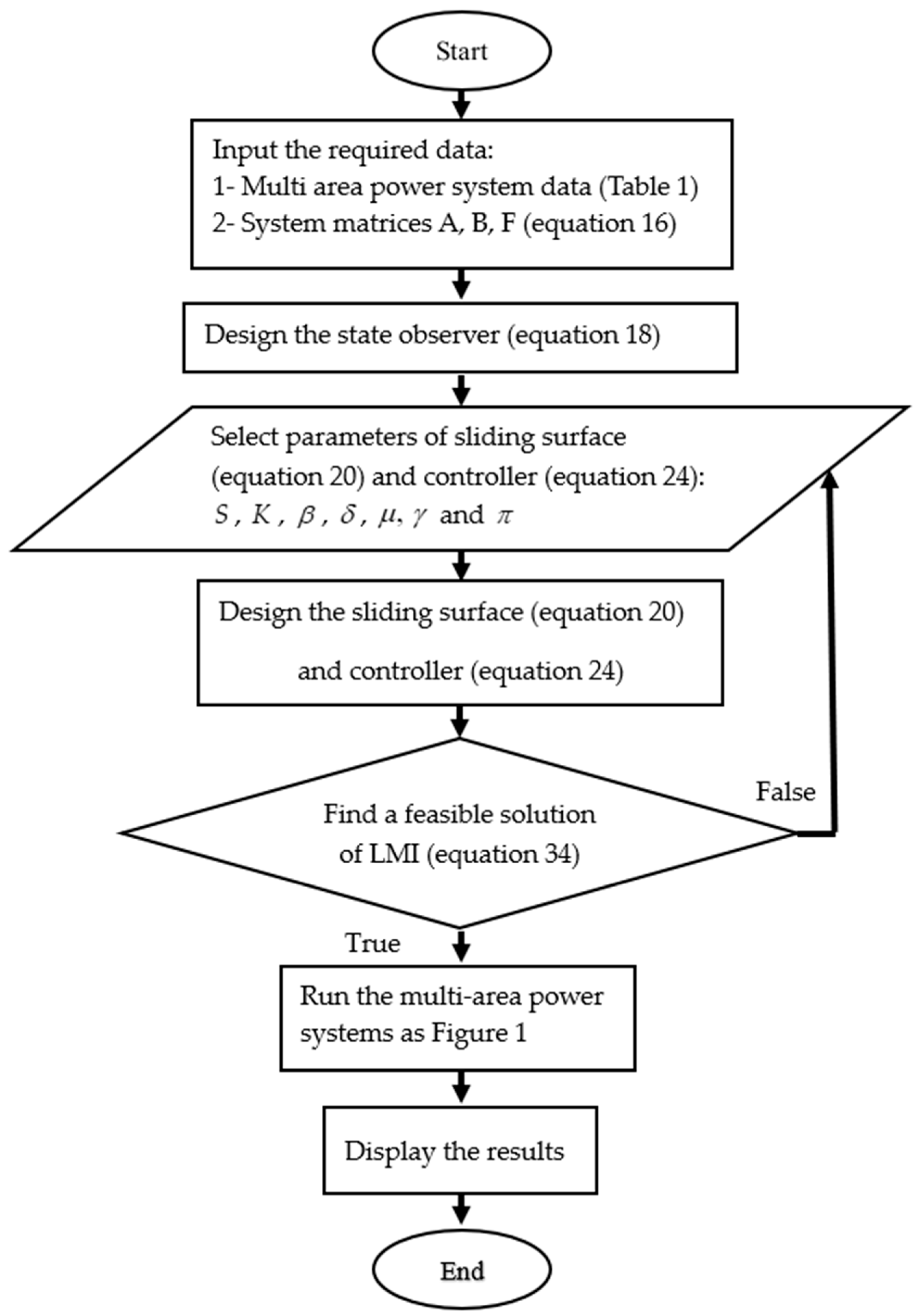
Therefore, Equation (44) indicates that V ˙ [ x ^ ( t ) ] < 0 which proves the reachability of the system states to the SPSS. Next, the flowchart of the proposed control algorithm of highly robust observer sliding mode can be implemented as Figure 2.
Remark 1.
The stability of the LFC in power system using LMI technique can be seen in [35]. However, the above approach needs to find four positive matrices in the LMI equations. Thus, the proposed approach only needs to find two positive matrices in LMI equations making it easier to find a feasible solution.

5. Simulation Results and Discussions

In this part, two simulations are done and the results are discussed and compared with other recent results.

5.1. Simulation 1

Parameters of the subsystem are obtained for simulation as given in [31] shown in Table 1.
The system matrices are calculated as
A = [ - 0 . 05 6 0 0 6 0 0 0 0 0 0 0 0 0 6 0 3.3 3.3 0 0 0 0 0 0 0 0 0 0 0 0 5.2 0 12.5 12.5 0 0 0 0 0 0 0 0 0 0 0 0.42 0 0 0 1 0 0 0 0 0 0 0 0 0 1 6.28 0 0 0 0 3.45 0 0 0 0 3.42 0 0 0 0 0 0 0 0 4.5 0.04 4.5 0 0 4.5 0 0 0 0 0 0 0 0 0 0 0 3.03 3.03 0 0 0 0 0 0 0 0 0 0 0 0 5.14 0 13.8 13.8 0 0 0 0 0 0 0 0 0 1 0.42 0 0 0 1 0 0 0 0 0 0 3.4 0 0 0 0 6.28 0 0 0 0 4.08 0 0 0 0 0 0 0 0 0 0 0 0 0 5.75 0.05 5.75 0 0 5.75 0 0 0 0 0 0 0 0 0 0 0 2.85 2.85 0 0 0 0 0 0 0 0 0 0 0 0 5.71 0 14.28 14.28 0 0 0 0 0 0 0 0 0 0 1 0.42 0 0 0 1 3.42 0 0 0 0 4.08 0 0 0 0 6.28 0 0 0 0 ]
The design parameters in the propose control are chosen to be β = 0.015 , μ = 1.3 ,
γ = 2.2 , ϑ = 2.2 , S = [ 0 0 12.5 0 0 0 0 0 0 0 0 0 0 0 0 0 0 0 0 0 0 0 13 . 89 0 0 0 0 0 0 0 0 0 0 0 0 0 0 0 0 0 0 0 14 . 28 0 0 ]
and
K = [ 172.5 58.8 5.3 401.9 592.8 5.7 0.8 0.07 427.6 731.7 10.4 1.4 0.04 1028 768 15.9 0.6 0.04 1498.8 1093.1 222.1 59.1 4.7 922.2 1125.2 13.1 2.6 0.11 979 1229 9.6 2.46 0.1 839 942.06 12.1 4.7 0.3 1127.5 1015.7 196.7 59.6 4.45 740 790 ]
By solving LMI (33), we have
R = [ 0.001 0 0 0.009 0 0 0 0 0 0 0 0 0 0 0 0 0 0 0 0 0 0 0 0 0.009 0 0 8.612 3.4 0.21 0.01 0 0 0 0 3.40 2.12 0.1 0.02 0 0.001 0 0 0.21 0.1 0.03 0.002 0 0 0 0 0.014 0.02 0 0.001 0 0 0 0 0.001 0 0 0 0 0.002 0 0 6.53 2.87 0.13 0.008 0 0 0 0 3.61 2.14 0.1 0.015 0 0 0 0 0.078 0.06 0 0 0 0 0 0 0.007 0.01 0 0 0 0 0 0 0 0 0 0 0 0.003 0 0 5.91 2.5 0.13 0.008 0 0 0 0 3.68 2.18 0.11 0.018 0 0.002 0 0 0 0 0.004 0 0 0 0 0 0 0 0 0 0 0 0 0 0 0 6.53 3.6 0.078 0.008 0 5.9 3.68 2.87 2.14 0.06 0.013 0 2.5 2.18 0.13 0.1 0 0 0 0.13 0.11 0 0.02 0 0 0 0.008 0.02 0 0 0 0 0 0 0 6.07 3.04 0.11 0.01 0 5.029 3.04 3.04 2.19 0.06 0.01 0 2.655 2.2 0.11 0.07 0.016 0.001 0 0.08 0.05 0.01 0.01 0.001 0.001 0 0.007 0.01 0 0 0 0 0 0 0 5.03 2.65 0.08 0.007 0 4.49 2.6 3.05 2.2 0.06 0.01 0 2.67 2.2 ] > 0
and
P = [ 0 0 0 0 0.01 0 0 0 0 0 0 0 0 0.01 0 0 15864 0 0.01 0 0 0 0 0.01 0 0 0.001 0 0 0 0 0 13564 0 0 0 0 0 0 0 0 0 0 0 0 0 0.01 0 11847 0.03 0.35 0.3 0 0.12 0.02 0.1 0.02 0 0.05 0.11 0.01 0 0 0.03 10516 0.22 0 0 0.36 0.3 0.1 0.02 0 0.21 0.2 0 0 0 0.35 0.22 0.06 0.01 0 0.13 0.16 0 0 0 0.1 0.13 0 0 0 0.028 0 0.011 8586 0 0.03 0.01 0 0.002 0 0 0 0 0 0 0.002 0 0 0 7865 0 0 0 0 0 0 0 0 0.01 0 0.12 0.36 0.13 0.02 0 7255 0.41 0.14 0.04 0 0.26 0.2 0 0 0 0.02 0.3 0.15 0.01 0 0.4 6733 0.12 0.02 0 0.2 0.18 0 0 0 0.12 0.14 0 0 0 0.14 0.12 0.03 0.006 0 0.07 0.07 0 0 0 0.02 0.02 0 0 0 0.03 0.02 0 5886 0 0.01 0 0 0 0 0 0 0 0 0 0 0 0 0 5538 0 0 0.01 0 0 0.05 0.21 0.11 0 0 0.26 0.2 0.07 0.01 0 5228 0.13 0 0 0 0.11 0.19 0.13 0 0 0.2 0.18 0.07 0.009 0 0.13 4952 ] > 0
Therefore, the LMI (33) is feasible.

5.1.1. Case 1

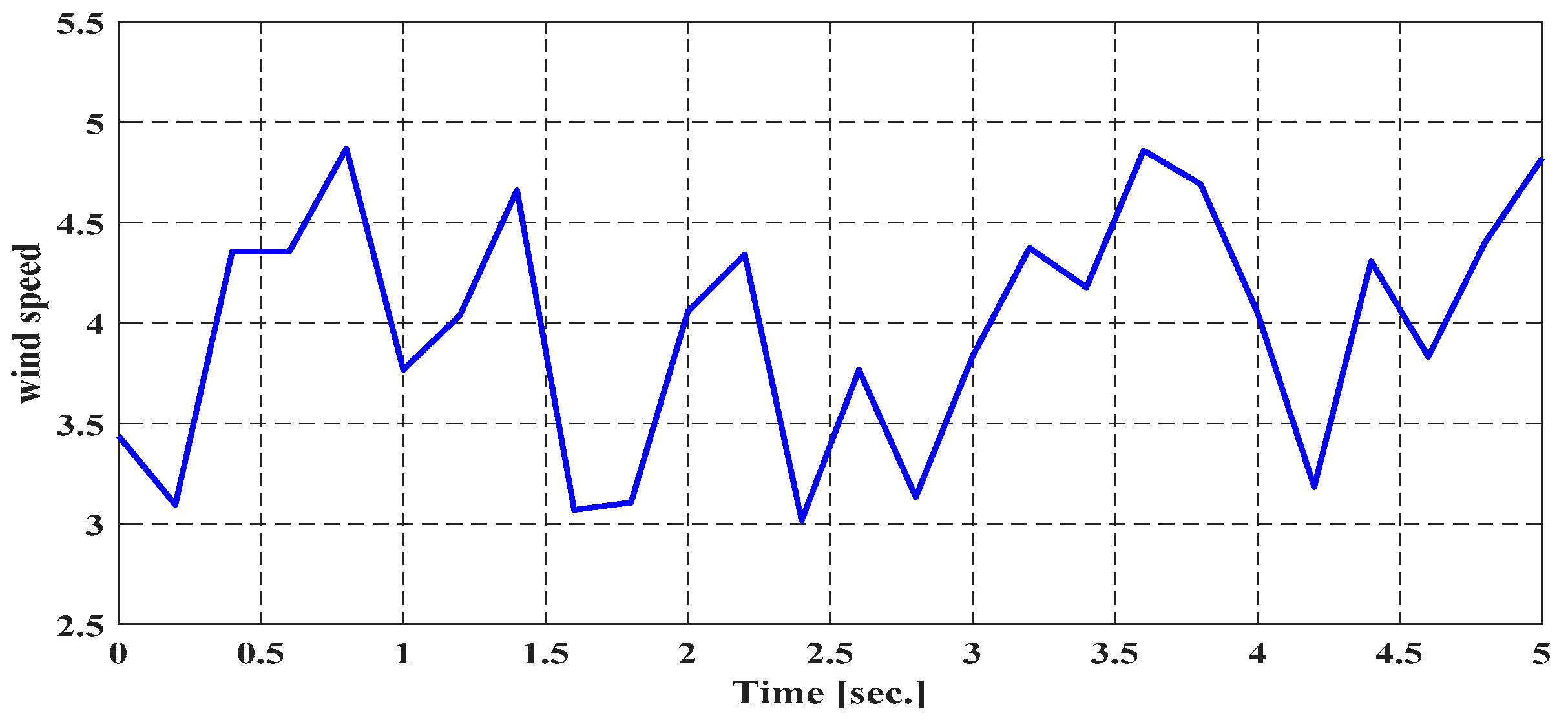
To examine the power system under the new algorithm, we apply step load changes with values of 0.01 p.u, 0.015 p.u and 0.02 p.u for Area 1, 2, and 3 together with wind speed variation in Figure 3. The respective results for incremental change in frequency and tie-flow distortion for the three areas are displayed in Figure 4 and Figure 5.
Both frequencies and tie-power flows spike at the initial point. At 2 s, the spikes are restored to zero point with lesser overshoots as compared to [31]. Table 2 gives a comparison result of both controllers. The single phase sliding surface without reaching time is used to cut-off the smaller overshoots.
Remark 2.
The power system response is seen better in terms of overshoots and settling time when compared with [31].

5.1.2. Case 2

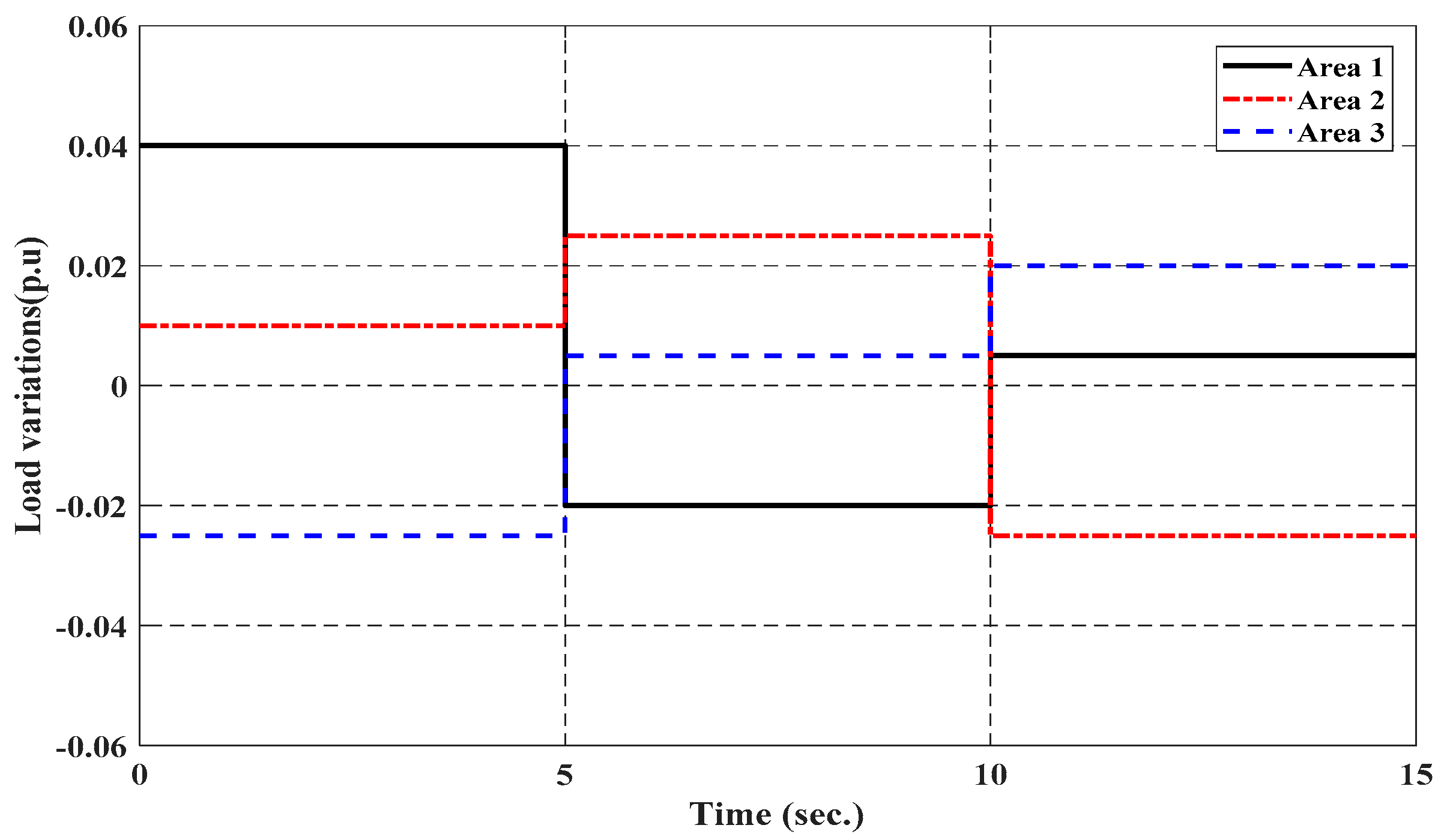
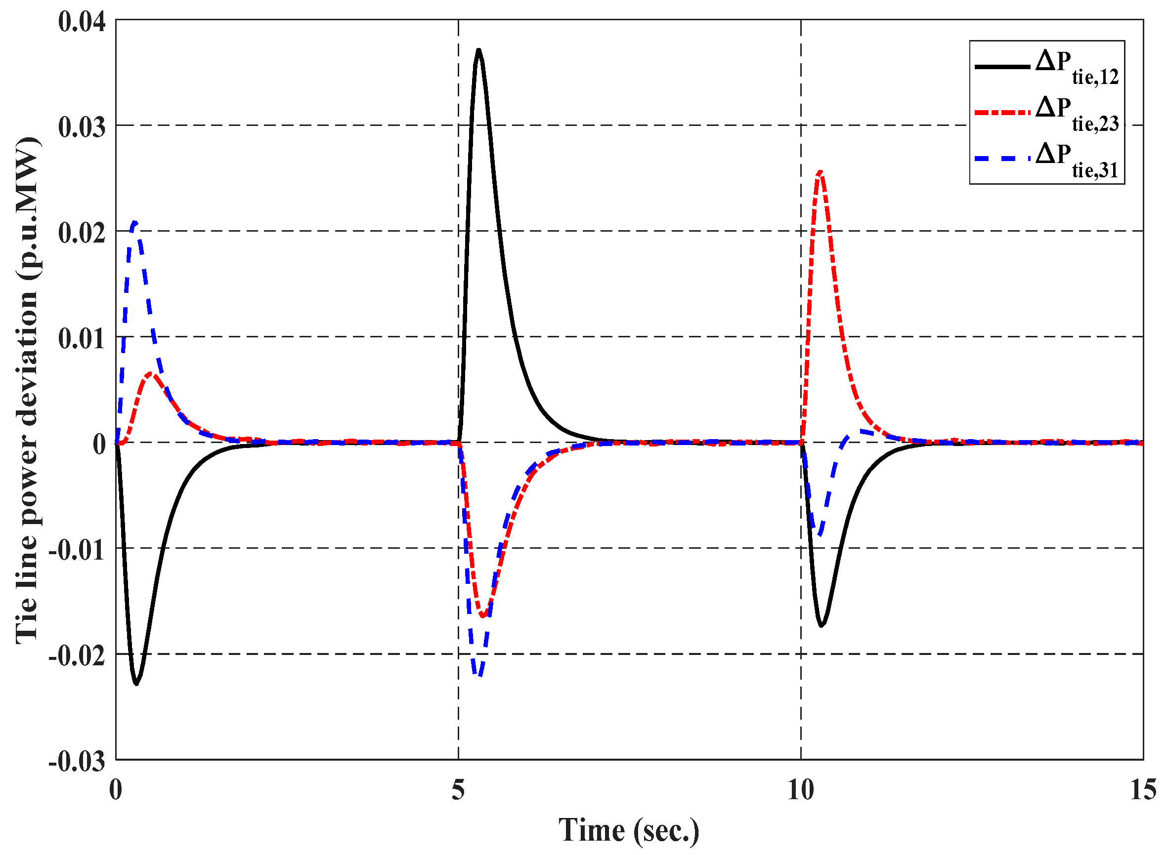
In reality, there is always continuous load demand from industries, households, etc., therefore, we assumed random load variations at every 5 s intervals as shown in Figure 6. We simulate again and the incremental frequency and tie-flow fluctuation for the three areas are shown in Figure 7 and Figure 8, accordingly. At this time, the new controller proves to be robust and converge the errors to zero at every interval without loss of control accuracies. The power system response is seen to be much better. This is to say the new controller provides good correction signal to adjust the reference load in the speed changer motor (non-reheat systems).
Remark 3.
The new controller robustness is validated against random load change and variable wind speed. It also proves to be applicable in real power system in terms of the smaller overshoots seen which do not have any significant effect as to cause wear and tear of the actuator valve.

5.2. Simulation 2

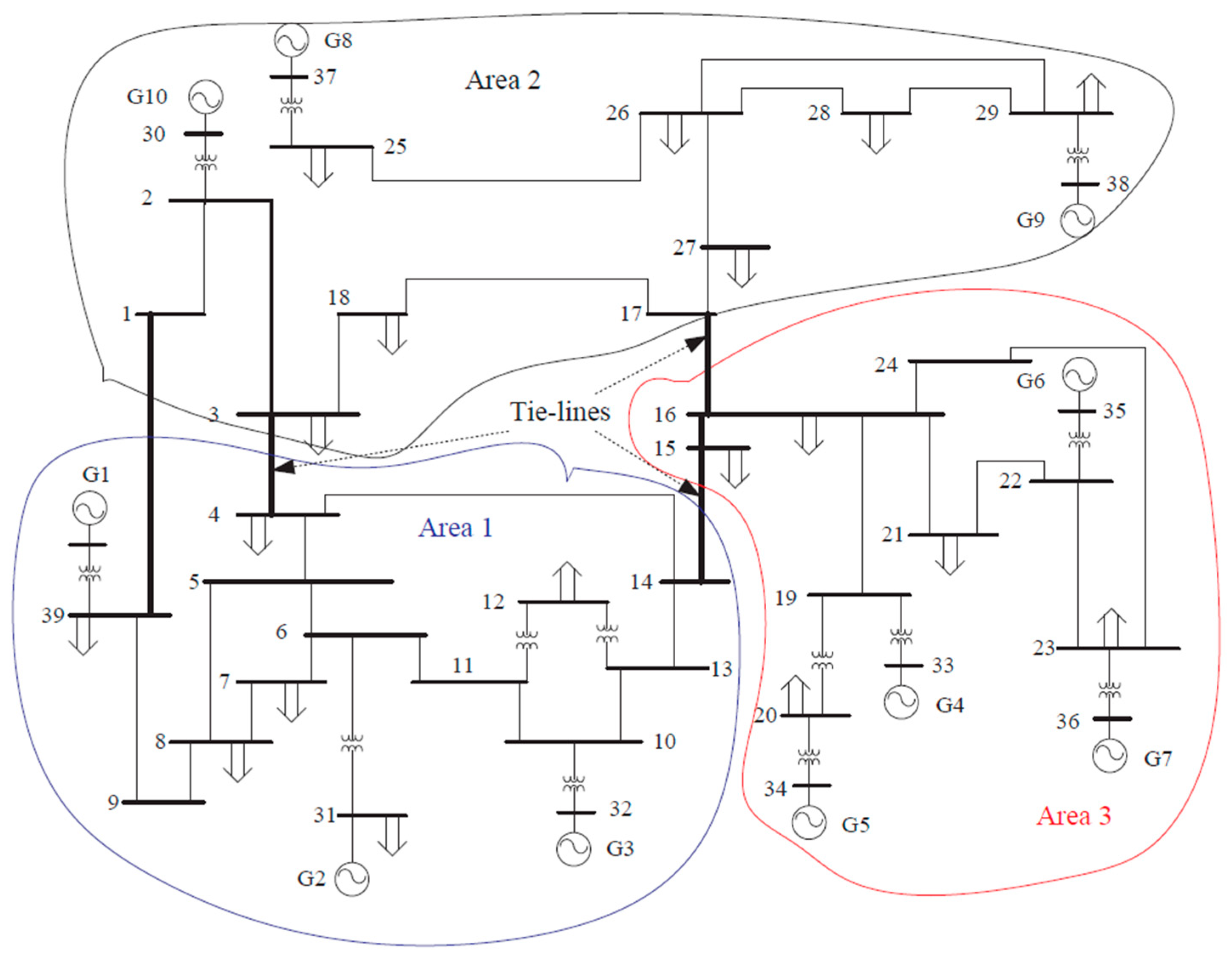
In this section, we simulate the performance of HROSM control design in a New England (IEEE 39 bus system) with parameters and the performance indices calculation shown in Table 3 as given in [36]. This system consists of 10 machines. The one-line diagram of the test system with its tie-line is displayed in Figure 9. Areas 1 and 2 have three generators, and there are four generators in Area 3; all generators are synchronized and operating in parallel running in a non-deregulated environment. The generators are equipped with governors. The total generated power and loads connected in Areas 1, 2 and 3 are 265.5, 233, 125 and 842 MW, respectively [36].
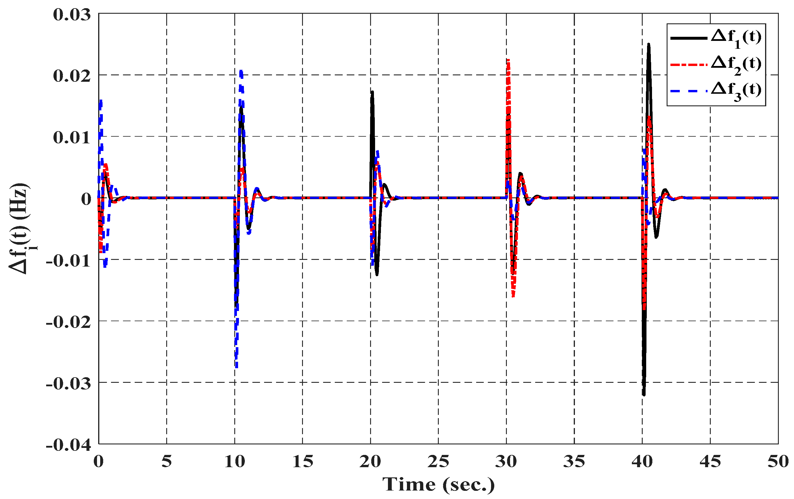
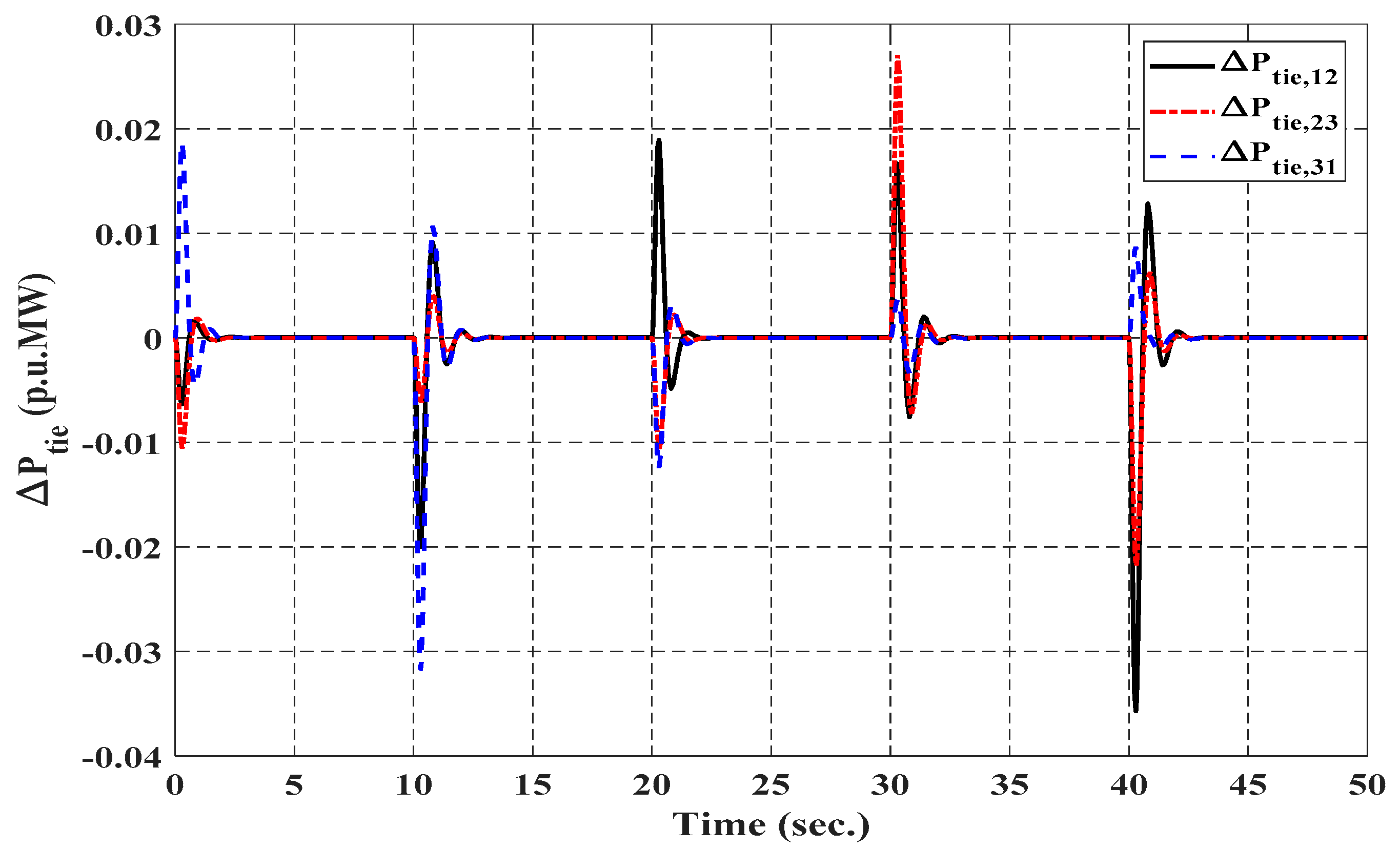
The New England system is simulated with the designed HROSM against variable load changes as shown in Figure 3. Figure 10 displayed the results of the frequency error of Area 3, while Figure 11 shows the tie-power exchange error results. In the results, it is seen that the new controller performance is good by damping the frequency and tie-power flow changes without loss of control and chattering free. The New England system response is better in terms of lesser settling time and overshoots which also cannot have any significant effect (i.e., wear and tear) on the governor steam actuator valve.
Remark 4.
It is seen that the new SPSS and the controller without reaching time keep frequency and tie-power flow at desired values in the New England 39 bus system with better response in overshoots and settling time. Therefore, this is the evidence that the new SPSS and controller without reaching time is good application for LFC of large power system.

6. Conclusions

In this paper, LFC problems in multi-area power integrated with renewable power plants is solved with proposed design of highly robust observer sliding mode via single phase switching. The proposed controller is designed to act only on the observer information and a single phase sliding is selected for SMC such that all estimated states trajectories begin at the surface at an initial time moment which makes it highly robust for applications. System stability is proved via the Lyapunov theory based on a new LMI scheme. Experimental simulation results show the new controller performed better when compared with recent SMC in terms of the rapid control of frequency and tie-flow spikes, and achieved chattering free without any weak control accuracies against external disturbances acting on the large multi-area power system. In addition, the proposed sliding surface and new controller, which depend on only the observer state estimation, are useful in applications for real power systems where all system state variables are difficult or expensive to measure.

Author Contributions

Conceptualization V.V.H., E.N.A.; Methodology P.T.T., A.-T.T., E.N.A.; Software A.-T.T., E.N.A.; Validation B.L.N.M., P.T.T.; Writing—original draft preparation E.N.A.; Writing—review and editing V.V.H.; Supervision B.L.N.M. All authors have read and agreed to the published version of the manuscript.

Funding

This research is funded by Foundation for Science and Technology Development of Ton Duc Thang University (FOSTECT), website: http://fostect.tdtu.edu.vn, under Grant FOSTECT.2017.BR.05.

Data Availability Statement

All data used is reported in the paper.

Conflicts of Interest

The authors declare no conflict of interest.

References

  1. Pandey, S.K.; Mohanty, S.R.; Kishor, N. A literature survey on load–frequency control for conventional and distribution generation power systems. Renew. Sustain. Energy Rev. 2013, 25, 318–334. [Google Scholar] [CrossRef]
  2. Thirunavukarasu, R.; Chidambaram, I. PI2 controller based coordinated control with Redox flow battery and unified power flow controller for improved restoration indices in a deregulated power system. Ain Shams Eng. J. 2016, 7, 1011–1027. [Google Scholar] [CrossRef]
  3. Farahani, M.; Ganjefar, S.; Alizadeh, M. PID controller adjustment using chaotic optimization algorithm for multi-area load frequency control. IET Control. Theory Appl. 2012, 6, 1984–1992. [Google Scholar] [CrossRef]
  4. Saxena, S.; Hote, Y.V. Decentralized PID load frequency control for perturbed multi-area power systems. Int. J. Electr. Power Energy Syst. 2016, 81, 405–415. [Google Scholar] [CrossRef]
  5. Yousef, H. Adaptive fuzzy logic load frequency control of multi-area power system. Int. J. Electr. Power Energy Syst. 2015, 68, 384–395. [Google Scholar] [CrossRef]
  6. Chaturvedil, D.K.; Satsangi, P.S.; Kalra, P.K. Load frequency control: A generalized neural network approach. Electr. Power Energy Syst. 1999, 21, 405–415. [Google Scholar] [CrossRef]
  7. Indulkar, C.S.; Raj, B. Application of fuzzy controller to automatic generation control. Electr. Mach. Power Syst. 1995, 23, 209–220. [Google Scholar] [CrossRef]
  8. Ghoshal, S.P. Multi area frequency and tie line power flow control with fuzzy logic based integral gain scheduling. J. Inst. Eng. 2003, 84, 135–141. [Google Scholar]
  9. Sinha, S.K.; Patel, R.N.; Prasad, R. Application of GA and PSO tuned fuzzy controller for AGC of three area thermal-thermal-hydro power system. Int. J. Comput. Theory Eng. 2010, 2, 238–244. [Google Scholar] [CrossRef]
  10. Juang, C.-F.; Lu, C.-F. Load-frequency control by hybrid evolutionary fuzzy PI controller. IEE Proc. Gener. Transm. Distrib. 2006, 153, 196–204. [Google Scholar] [CrossRef]
  11. Arya, Y.; Kumar, N. BFOA-scaled fractional order fuzzy PID controller applied to AGC of multi-area multi-source electric power generating sys-tems. Swarm Evol. Comput. 2017, 32, 202–218. [Google Scholar] [CrossRef]
  12. Fathy, A.; Kassem, A.M.; Abdelaziz, A.Y. Optimal design of fuzzy PID controller for deregulated LFC of multi-area power system via mine blast algorithm. Neural Comput. Appl. 2018, 32, 4531–4551. [Google Scholar] [CrossRef]
  13. Haroun, A.G.; Li, Y. A novel optimized hybrid fuzzy logic intelligent PID controller for an interconnected multi-area power system with physical constraints and boiler dynamics. ISA Trans. 2017, 71, 364–379. [Google Scholar] [CrossRef] [PubMed]
  14. Kouba, N.E.Y.; Menaa, M.; Hasni, M.; Boudour, M. Load frequency control in multi-area power system based on Fuzzy Logic-PID Controller. In Proceedings of the 2015 IEEE International Conference on Smart Energy Grid Engineering (SEGE), Oshawa, ON, Canada, 17–19 August 2015; pp. 1–6. [Google Scholar]
  15. Sahu, R.K.; Panda, S.; Yegireddy, N.K. A novel hybrid DEPS optimized fuzzy PI/PID controller for load frequency control of multi-area intercon-nected power systems. J. Process. Control. 2014, 24, 1596–1608. [Google Scholar] [CrossRef]
  16. Jagatheesan, K.; Anand, B.; Samanta, S.; Dey, N.; Ashour, A.S.; Balas, V.E. Design of a proportional-integral-derivative controller for an automatic generation control of multi-area power thermal systems using firefly algorithm. IEEE/CAA J. Autom. Sin. 2017, 6, 503–5151. [Google Scholar] [CrossRef]
  17. Mohapatra, T.K.; Sahu, B.K. Design and implementation of SSA based fractional order PID controller for automatic generation control of a multi-area, multi-source interconnected power system. In Proceedings of the Technologies for Smart-City Energy Security and Power (ICSESP), Bhubaneswar, India, 28–30 March 2018; pp. 1–6. [Google Scholar]
  18. Raju, M.; Saikia, L.C.; Sinha, N. Automatic generation control of a multi-area system using ant lion optimizer algorithm based PID plus second order derivative controller. Int. J. Electr. Power Energy Syst. 2016, 80, 52–63. [Google Scholar] [CrossRef]
  19. Jianping, G. Sliding Mode Based Load Frequency Control for an Interconnected Power System with Nonlinearities. Ph.D. Thesis, Cleveland State University, Cleveland, OH, USA, 2015. [Google Scholar]
  20. Vrdoljak, K.; Perić, N.; Petrović, I. Sliding mode based load-frequency control in power systems. Electr. Power Syst. Res. 2010, 80, 514–527. [Google Scholar] [CrossRef]
  21. Prasad, S.; Purwar, S.; Kishor, N. Non-linear sliding mode control for frequency regulation with variable-speed wind turbine systems. Int. J. Electr. Power Energy Syst. 2019, 107, 19–33. [Google Scholar] [CrossRef]
  22. Trip, S.; Cucuzzella, M.; De Persis, C.; van der Schaft, A.; Ferrara, A. Passivity-based design of sliding modes for optimal load frequency control. IEEE Trans. Control. Syst. Technol. 2018, 27, 1893–1906. [Google Scholar] [CrossRef] [Green Version]
  23. Huynh, V.V.; Tsai, Y.-W.; Duc, P.V. Adaptive output feedback sliding mode control for complex interconnected time-delay systems. Math. Probl. Eng. 2015, 1–15. [Google Scholar] [CrossRef] [Green Version]
  24. Lee, S.-W.; Chun, K.-H. Adaptive sliding mode control for PMSG wind turbine systems. Energies 2019, 12, 595. [Google Scholar] [CrossRef] [Green Version]
  25. Lv, X.; Sun, Y.; Wang, Y.; Dinavahi, V. Adaptive event-triggered load frequency control of multi-area power systems under networked environ-ment via sliding mode control. IEEE Access 2020, 8, 86585–86594. [Google Scholar] [CrossRef]
  26. Le Ngoc Minh, B.; Van Huynh, V.; Nguyen, T.M.; Tsai, Y.W. Decentralized adaptive double integral sliding mode controller for multi-area power systems. Math. Probl. Eng. 2018, 2018, 1–11. [Google Scholar] [CrossRef]
  27. Guo, J. Application of full order sliding mode control based on different areas power system with load frequency control. ISA Trans. 2019, 92, 23–34. [Google Scholar] [CrossRef] [PubMed]
  28. Sarkar, M.K.; Dev, A.; Asthana, P.; Narzary, D. Chattering free robust adaptive integral higher order sliding mode control for load frequency problems in multi-area power systems. IET Control. Theory Appl. 2018, 12, 1216–1227. [Google Scholar] [CrossRef]
  29. Dev, A.; Sarkar, M.K.; Asthana, P.; Narzary, D. Event-triggered adaptive integral higher-order sliding mode control for load frequency problems in multi-area power systems. Iran. J. Sci. Technol. Trans. Electr. Eng. 2019, 43, 137–152. [Google Scholar] [CrossRef]
  30. Hu, R.; Deng, H.; Zhang, Y. Novel dynamic-sliding-mode-manifold-based continuous fractional-order nonsingular terminal sliding mode control for a class of second-order nonlinear systems. IEEE Access 2020, 8, 19820–19829. [Google Scholar] [CrossRef]
  31. Dev, A.; Sarkar, M.K. Robust higher order observer based non-linear super twisting load frequency control for multi area power systems via sliding mode. Int. J. Control. Autom. Syst. 2019, 17, 1814–1825. [Google Scholar] [CrossRef]
  32. Prasad, S.; Purwar, S.; Kishor, N. Load frequency regulation using observer based non-linear sliding mode control. Int. J. Electr. Power Energy Syst. 2019, 104, 178–193. [Google Scholar] [CrossRef]
  33. Tsai, Y.W.; Van, H.V. Adaptive Output Feedback Control for Mismatched Uncertain Systems: Single Phase Sliding Mode Approach. In Proceedings of the International Symposium on Computer, Consumer and Control, Taichung, Taiwan, 10–12 June 2014; pp. 990–993. [Google Scholar]
  34. Boyd, S.; El Ghaoui, L.; Feron, E.; Balakrishnan, V. Linear Matrix Inequalities in System and Control Theory; Society for Industrial and Applied Mathematics (SIAM): Philadelphia, PA, USA, 1994. [Google Scholar]
  35. Manikandan, S.; Kokil, P. Stability analysis of load frequency control system with constant communication delays. IFAC Papersonline 2020, 53, 338–343. [Google Scholar] [CrossRef]
  36. Liao, K.; Xu, Y. A robust load frequency control scheme for power systems based on second-order sliding mode and extended disturbance observer. IEEE Trans. Ind. Inform. 2017, 14, 3076–3086. [Google Scholar] [CrossRef]
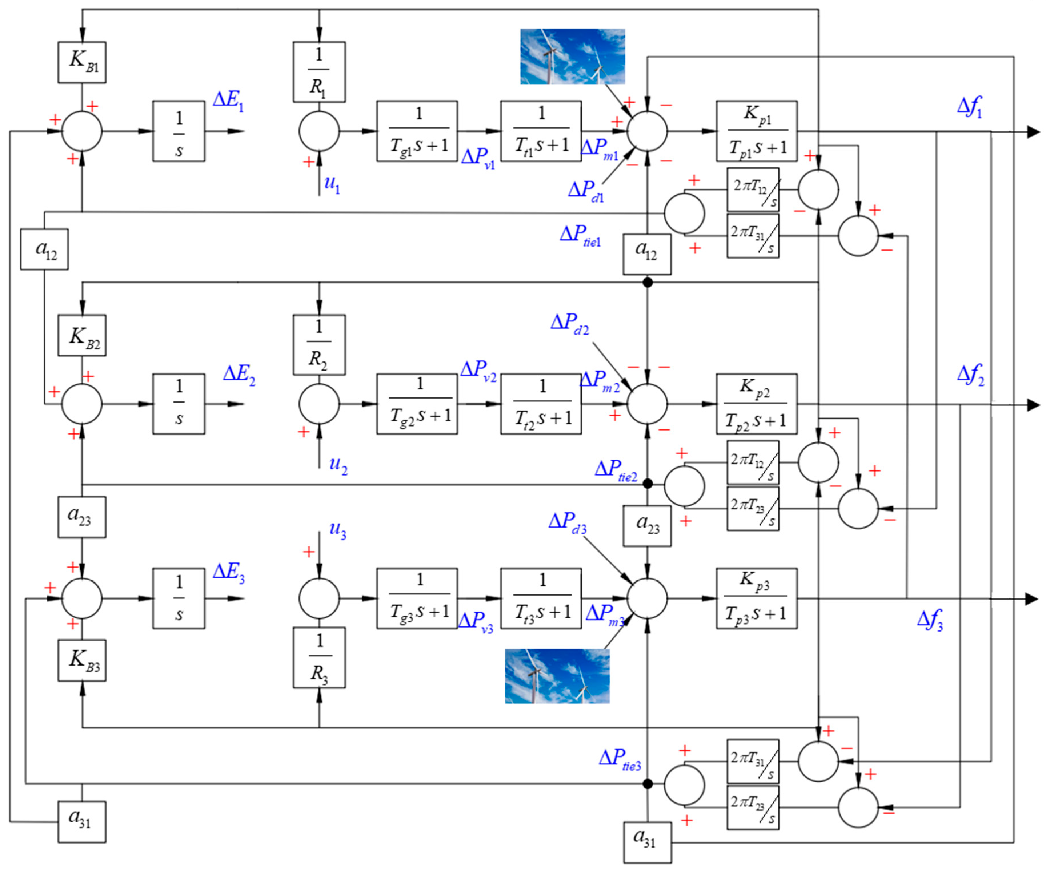
Figure 1. Block diagram of 3-area LFC (load frequency control) system with renewables.
Electronics 10 00274 g001
Figure 2. The flowchart of the proposed highly robust observer sliding mode based load frequency control.
Electronics 10 00274 g002
Figure 3. Wind speed (m/s).
Electronics 10 00274 g003
Figure 4. Frequency spikes against step load disturbance and wind speed variation.
Electronics 10 00274 g004
Figure 5. Tie-line power deviation.
Electronics 10 00274 g005
Figure 6. Load variations of three areas.
Electronics 10 00274 g006
Figure 7. Frequency spikes against load variations.
Electronics 10 00274 g007
Figure 8. Tie-line power deviation.
Electronics 10 00274 g008
Figure 9. The New England IEEE 39 bus power system.
Electronics 10 00274 g009
Figure 10. Frequency deviation of three areas.
Electronics 10 00274 g010
Figure 11. Tie-line power deviation.
Electronics 10 00274 g011
Table 1. Power system parameters.
Parameters T P i K P i T T i T G i R i
Area 1201200.30.082.4
Area 225112.50.330.0722.7
Area 3201150.350.072.5
Table 2. Setting time T s and Maximum Overshoot (M.O.S).
Proposed HROSM
via Single Phase Sliding Surface
The Approach Given in [31]
Frequency ErrorsSettling Time
T s [s]
Max.O. S
[pu]
Settling Time T s [s]Max.O. S
[pu]
Δ f 1 1.50.00320.005
Δ f 2 1.50.001920.003
Δ f 3 1.50.001920.003
HROSM: highly robust observer sliding mode.
Table 3. Parameters of the New England IEEE 39 bus power system.
Generations
(bus No.)
M (Moment of Inertia of the Generator)D (Generator’s Damping Rations) T g (Governor Time Constant) T T (Turbine-Generator Time Constant) Linearization Parameter of the Governor Characteristic
K t e T r
G1 (39)3.04.00.250.225039.419
G2 (31)2.54.00.250.225039.419
G3 (32)4.06.00.250.225039.419
G4 (33)2.03.50.250.225039.419
G5 (34)3.53.00.250.225039.419
G6 (35)3.07.50.250.225039.419
G7 (36)2.54.00.250.225039.419
G8 (37)2.06.50.250.225039.419
G9 (38)6.05.00.250.225039.419
G10 (30)4.05.00.250.225039.419
Publisher’s Note: MDPI stays neutral with regard to jurisdictional claims in published maps and institutional affiliations.