Article

Edge Computing for Data Anomaly Detection of Multi-Sensors in Underground Mining

School of Computer Science and Engineering, Northeastern University, Shenyang 110819, China
*
Author to whom correspondence should be addressed.
Electronics 2021, 10(3), 302; https://doi.org/10.3390/electronics10030302
Submission received: 24 December 2020 / Revised: 10 January 2021 / Accepted: 23 January 2021 / Published: 27 January 2021

Abstract

:
There is a growing interest in safety warning of underground mining due to the huge threat being faced by those working in underground mining. Data acquisition of sensors based on Internet of Things (IoT) is currently the main method, but the data anomaly detection and analysis of multi-sensors is a challenging task: firstly, the data that are collected by different sensors of underground mining are heterogeneous; secondly, real-time is required for the data anomaly detection of safety warning. Currently, there are many anomaly detection methods, such as traditional clustering methods K-means and C-means. Meanwhile, Artificial Intelligence (AI) is widely used in data analysis and prediction. However, K-means and C-means cannot directly process heterogeneous data, and AI algorithms require equipment with high computing and storage capabilities. IoT equipment of underground mining cannot perform complex calculation due to the limitation of energy consumption. Therefore, many existing methods cannot be directly used for IoT applications in underground mining. In this paper, a multi-sensors data anomaly detection method based on edge computing is proposed. Firstly, an edge computing model is designed, and according to the computing capabilities of different types of devices, anomaly detection tasks are migrated to different edge devices, which solve the problem of insufficient computing capabilities of the devices. Secondly, according to the requirements of different anomaly detection tasks, edge anomaly detection algorithms for sensor nodes and sink nodes are designed respectively. Lastly, an experimental platform is built for performance comparison analysis, and the experimental results show that the proposed algorithm has better performance in anomaly detection accuracy, delay, and energy consumption.

1. Introduction

At present, the underground mining method has been adopted in many mines, especially metal mines. However, during the underground construction process, toxic gases, water gushing-out, and mine collapse pose huge threats to the safety of construction workers [1,2]. Therefore, risk monitoring and the early warning of underground construction process is of great significance. Internet of Things (IoT) technology can use sensors to collect data, transmitting data through Wireless Sensor Networks (WSNs), and process the data at the terminal. Therefore, IoT technology is widely used in underground mining construction safety monitoring and early warning [3].
The purpose of the underground mining construction safety monitoring that is based on IoT is to detect anomalies in the data that are collected by the sensors, through which safety assessment can be carried out. For an abnormal data, through algorithmic analysis, the type and source of the abnormality can be determined. In underground mining, many reasons, such as sensor failures, environmental changes, and wireless data interference, can cause data abnormalities. Therefore, comprehensive analysis is required. There are different types of sensors, such as CO 2 , gas, and so on, by which the data are generated and transmitted to the cloud server through the sink nodes and the forwarding device. In the cloud, after data analysis, the construction environment can be grasped in a timely, effective, and comprehensive manner, thereby effectively preventing the occurrence of mine accidents.
There are many research results for the abnormal detection of sensor data. In underground mines, the main research work is to detect data anomalies based on the characteristics of the complex environment underground, and periodic alarms can be used instead of static alarm threshold settings. In addition, the lack of a large amount of empirical data is the relevant research difficulty of underground data anomaly detection, which makes the effective application of artificial intelligence and other methods impossible. Muduli et al. [4] proposed an optimized fuzzy logic-based fire monitoring system for a wireless underground sensor network, which strengthens the reliability of making decision in preventing mine fire. The binary particle swarm optimization (BPSO) algorithm was used to optimize the proposed fuzzy system that eliminates redundant rules, but preserves event detection accuracy of the monitoring system. The simulation results demonstrate that the proposed system outperforms the existing monitoring systems for underground coal mines. Mishra et al. [5] fully analyzed the importance of methane monitoring for coal mine safety, and maked an attempt to develop a model for predicting methane concentration in underground coal mines based on seven different geo-mining factors while using multi-layered artificial neural networks. This study‘s objective was to quantify the relative influences of these factors on methane dispersion in underground coal mines and identify the significant factors through sensitivity analysis. The outcome of this study was useful in designing a mine ventilation system for effective coal mine methane management and enhancing mines safety. Zhang et al. [6] obtained 28 representative risk factors and 16 coupled types of risk factors through the analysis of 332 gas explosion accidents in coal mines in China. An eight-level hierarchical model of risk coupling of a gas explosion accident was established through the application of the combined ISM-NK model, and the coupled degrees of different types of risk coupling were assessed. A quantitative analysis of the NK model shows that the probability of gas explosion increases with the increasing number of risk factors. When compared with subjective risk factors, objective risk factors have a higher probability of causing gas explosion due to risk coupling. Vaziri et al. [7] proposed a geological–geotechnical risk assessment model for the identification of high risk-prone areas in underground coal mines while using an integrated GIS-geostatistics system. This study chose Tabas, which was the first mechanized and largest underground coal mine in Iran as a case study. The geostatistics module in ArcGIS was used for estimating the amount of coal seam gas content, CMRR, and initial in situ stress in unstamped areas, as well as providing the prediction maps. Additionally, a rock engineering system-–interaction matrix method was used for attribute weight assignment. The analysis results of final risk map indicated that approximately 45 of under study area is prone to high to very high geohazards risk.
However, many existing research results cannot be directly applied to underground data anomaly detection. The main reasons are:
  • The sensor data in underground mining have very obvious time series characteristics, and the data collected by the sensor vary with time, depending on the construction environment in underground mining.
  • Most of the underground construction operation environment is in the tunnel, of which the space is small, but the operation distance is long. Therefore, a large number of sensors need to be deployed in different areas, and there is a correlation between the sensor data at different locations.
Therefore, in underground mining, anomaly detection is required for multi-sensor data. In addition, for any type of sensor data, most of the existing methods are to process it on a cloud server, which brings some problems: firstly, a lot of invalid and redundant data transmission will waste a limited network resources; secondly, some sensor data have real-time requirements for anomaly detection, such as toxic gas sensor data. When the data are abnormal, it is necessary to detect the anomaly type as soon as possible and then make an early warning in time. Therefore, the transmission of data to the cloud for processing will cause delay, which reduces the real-time performance of data anomaly detection.
In order to solve the existing problems, increasing studies have begun to consider migrating data processing tasks in the cloud to different terminal devices for processing. This edge computing idea is very consistent with the needs of data anomaly detection in underground mining. An edge computing-based multi-sensor data anomaly detection scheme in underground mining is proposed, which transfers part of the task of data anomaly detection to sink nodes and sensor nodes for execution. The main contributions are as follows:
  • An anomaly detection task migration model is proposed to migrate data anomaly detection tasks to different types of equipment for execution.
  • An anomaly detection method for sensor nodes is designed that is based on K-means and C-means algorithms. An anomaly detection algorithm based on ambiguity is proposed in order to perform anomaly detection and data clustering analysis on the redundant data collected by the sensor.
  • An anomaly detection method of the sink node is designed for preprocessing the multi-sensors’ data, and then use the sliding window to analyze the time series of the multi-sensors’ data in order to obtain the anomaly detection results.
The rest of the work is organized, as follows: Section 2 discusses the related work of this paper. Section 3 introduces the anomaly detection model of wireless sensor data in underground mining, and it proposes an anomaly detection task migration model that is based on edge computing. Section 4 proposes data anomaly detection schemes for the sensor node and the sink node, respectively. Section 5 presents an experimental analysis. Section 6 concludes the work of this paper.

2. Related Work

At present, the methods of anomaly detection are mainly divided into clustering methods, statistical methods, AI methods, and so on [8,9,10,11,12]. The goal of most studies is to improve accuracy, and less consideration is given to indicators, such as energy consumption and delay.

2.1. Clustering-Based Methods

Clustering is an effective anomaly detection method, which includes many traditional algorithms, such as K-means [13] and C-means [14]. There are a lot of algorithms improved based on these classic algorithms. At present, cluster-based anomaly detection methods are still one of the main research directions [15], especially when AI technology is increasingly widely used; many clustering algorithms have begun to be applied in this field.
Habeeb et al. [16] proposed a real-time anomaly detection framework that is based on big data technology. In addition, a streaming sliding window local outlier factor coreset clustering algorithms (SSWLOFCC) was developed, and then implemented into the framework. The experimental results verify its performance in terms of accuracy, memory consumption, and execution time. Ilia Nouretdinov et al. [17] presented a clustering technique, called multi-level conformal clustering (MLCC), which was hierarchical in nature, because it can be performed at multiple significance levels, which yields greater insight into the data than performing it at just one level. There were several advantages of using MLCC over more classical clustering techniques: once a significance level has been set, MLCC was able to automatically select the number of clusters. Furthermore, thanks to the conformal prediction framework, the resulting clustering model has a clear statistical meaning without any assumptions regarding the distribution of the data. Ghezelbash et al. [18] believed that, due to the complicated characteristics of regional geochemical data from stream sediments as a result of the complexity of geological features, the detection of multi-elemental geochemical footprints of mineral deposits of interest was a challenging task. To address this, a hybrid genetic algorithm-based technique, namely the genetic K-means clustering (GKMC) algorithm, was proposed for the optimum delineation of multi-elemental patterns (both anomaly and background) in stream sediment geochemical data. Huang et al. [19] proposed a density peak (DP)-weighted fuzzy C-means (WFCM) based clustering method, which was used to detect abnormal situations in the production process. A real case from an IoT enabled machining workshop was carried out in order to verify the accuracy and effectiveness of the proposed method in the anomaly detection of manufacturing process. Bilal et al. [20] proposed a hybrid anomaly detection method for misdirection and black hole attacks by employing customized clustering technique. Experimental work was performed on network simulator (NS-2) and R studio, which showed it to be suitable for hybrid anomaly detection, including misdirection and black hole attacks in wireless environment. Nguyen et al. [21] proposed a road anomaly detection method while using the Grubbs test on a sliding window to make it adaptive to the local characteristics of the road. This method included a clustering algorithm and a mean shift-based algorithm to aggregate reported anomalies on data to the server. Aggarwal et al. [22] proposed a hybrid of proximity-based and clustering-based anomaly detection approaches to identify anomalies in the air quality data. The Gaussian distribution property of the real-world data set was further utilized to segregate out anomalies. The results showed that the proposed method can be efficient in the extraction of anomalies and can increase the accuracy by reducing the number of false alarms.

2.2. AI-Based Methods

Anomaly detection methods can be categorized into distance-based, cluster-based, classification-based, and statistical anomaly detection methods. Additionally, AI is now increasingly applied to anomaly detection. Machine learning is an important method, in which deep learning and neural networks are widely used in various application scenarios that require empirical analysis [23].
Quatrini et al. [24] proposed a two-step methodology for anomaly detection in industrial processes based on machine learning classification algorithms. Starting from the real-time collection of process data, the first step identifies the ongoing process phase, the second step classifies the input data as “Expected”, “Warning”, or “Critical”. This methodology applies the decision forests algorithm, as a well-known anomaly detector from industrial data, and decision jungle algorithm, which has never been tested before in industrial applications. Park et al. [25] proposed a multi-labeled hierarchical classification (MLHC) intrusion detection model that analyzes and detects external attacks that are caused by message injection. This model quickly determines the occurrence of attacks and classifies the attack using only existing classified attack data, which can classify both the type and existence or absence of attacks with high accuracy and it can be used in interior communication environments of high-speed vehicles with a high throughput. Tsukada et al. [26] proposed ONLAD and its IP core, named ONLAD Core, which is highly optimized in order to perform fast sequential learning to follow concept drift in less than one millisecond. ONLAD Core realizes on-device learning for edge devices at low power consumption, which realizes standalone execution where data transfers between edge and server are not required. Tang et al. [27] proposed an anomaly detection neural network, dual auto-encoder generative adversarial network (DAGAN), which was developed to solve the problem of sample imbalance. With skip-connection and dual auto-encoder architecture, the proposed method exhibited excellent image reconstruction ability and training stability.

3. System Model

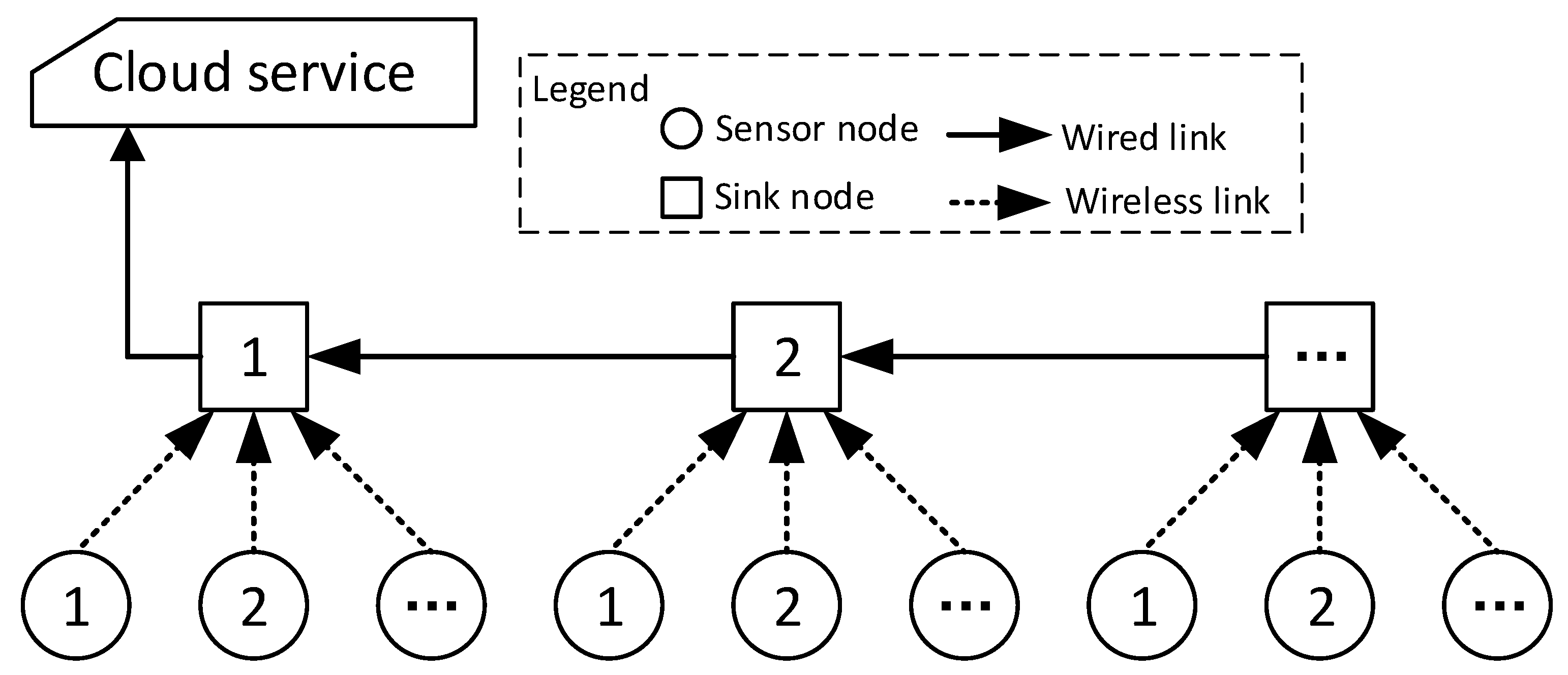
3.1. Application Model of IoT in Underground Mining

IoT has been increasingly used to monitor the safety of the construction environment in underground mining. The sensors are used to collect, aggregate, and transmit data, and then perform data anomaly detection. At present, the data transmission in underground mining is realized through WSNs. Sensors make the environmental data acquisition, and it is send to the sink device and then forwarded to the monitoring center in the cloud.
Figure 1 shows a typical data transmission model of IoT in underground mining. There are three types of equipment for the IoT in underground mining: cloud server, sink node, and sensor node. A sensor node collects all kinds of environmental data according to requirements. There are many different types of sensors, and the data of these sensors are heterogeneous. The data that are collected by the sensors will be sent to the sink node through the wireless link. A sink node can usually receive the data sent by multiple sensors, and then forward these data to the cloud server through a wired link (because the sink node in underground mining is deployed according to the tunnel structure. Therefore, chained topology is a common structure [28]). The cloud server stores the received data, and then analyzes and processes it as needed.
The purpose of data anomaly detection in this article is to determine whether there is an abnormality in the current construction environment based on the analysis of the data, and to provide timely early warning. If data anomaly detection is performed in the remote cloud server, then data transmission will cause a large delay, which results in untimely early warning. Therefore, edge computing, which is migrating data anomaly detection tasks to the edge, is a good choice [29]. However, the computing and storage capabilities of underground IoT devices are limited, and complex calculations cannot be performed. Therefore, the task of data anomaly detection needs to be divided into several parts and migrated to different edge devices for execution.
In underground mining, there are two types of edge devices: sink node and sensor node. A sensor node is equipment for data collection and data preprocessing, and a sink node is equipment for data aggregation, fusion, and forwarding. In this article, according to the data’s characteristics of the underground environment, the data anomaly detection task will be reasonably migrated to the sensor node and the sink node.

3.2. Edge Computing Model of Anomaly Detection

In underground mining, the data are collected and sent by sensors, processed by the sink node, and then forwarded. An edge computing model for anomaly detection task migration is proposed to improve the real-time of anomaly detection.
The sensor’s data acquisition is periodic, so it has the characteristics of time series, and it is necessary to analyze the data within a period of time. In addition, multiple sensors of the same type are distributed in different locations because the underground tunnel is long. The data in different locations have correlation, and it is necessary to comprehensively judge the abnormal situation of the data.
Chandola et al. [30] divided data anomalies into three categories: Point Anomalies, Contextual Anomalies, and Collective Anomalies. According to the actual needs of underground construction, this article divides the anomalies into two categories:
  • Data corruption.
    It means that after the collected data are distorted due to equipment failure, battery loss, etc., which cannot represent the true data value. For example, when a sensor’s battery power is less than the standard value, the data that it collects will cause errors. However, this error is not a true data anomaly.
  • Data anomaly.
    It refers to the abnormality of the underground construction environment that is shown by the real data value, such as the decrease of oxygen concentration, which indicates that there may be problems with the ventilation system. According to the definition of [30], the data anomalies in this article include three cases:
    • Point Anomalies
      If a sensor data value does not meet the range of the normal data value, it is judged as Point Anomalies. For example, if a temperature value is found to be greater than 40, then it is considered that the underground environment at this temperature is abnormal. However, there are correlations between different types of sensors in the mine, such as temperature and humidity sensors. Therefore, the Point Anomalies of a single sensor cannot truly reflect the actual environmental anomalies.
    • Contextual Anomalies
      In underground mining, if there are abnormalities in different correlated sensors, then it can be considered that the environment is abnormal under the current conditions. However, due to the deployment of automatic sprinkler, emergency ventilation and other equipment, Contextual Anomalies can only indicate that the environment in underground mining is abnormal at a certain moment, and it is likely that the emergency equipment will start at the next moment, which makes the environment start to become normal. In this case, it cannot be defined as an environmental abnormality and an emergency warning is activated.
    • Collective Anomalies
      In a period of time, if multiple consecutive Contextual Anomalies occur, it can be considered to be a collective anomalies.
Real-time performance cannot be guaranteed if anomaly detection tasks are executed in the cloud. In the underground construction environment, the sink node will use the equipment, such as buzzer, to give early warning for environmental anomalies. Therefore, sending the data to the cloud and then returning to the sink node will cause a large delay. For example, the sink node sends the collected data to the cloud. Because the cloud is usually deployed on the ground or even a faraway server center, this will lead to a long data transmission time. In addition, cloud servers usually use AI algorithms for data anomaly detection, of which the execution time will be longer. If an abnormality is found, then an early warning will be given or the emergency equipment under the mine will be notified to start. The server that is deployed in the cloud can complete the task of data anomaly detection, but it will take more time, which leads to missing the best time for emergency rescue work in some cases. Therefore, the current approach is to deploy equipment under the mine to detect data anomalies, and to provide early warning that is based on the detection results in a timely manner. However, due to the limited CPU’s computing power of the sink node, it cannot process the analysis of a large amount of data, especially the safety prediction of the construction environment. Therefore, some anomaly detection tasks have to be migrated to the cloud for processing. As shown in Figure 2, this article divides the anomaly detection task into three parts:
  • Cluster analysis.
    The sensor node performs cluster analysis. The sensor node analyzes whether the data value is abnormal according to the received data. It is mainly to determine whether the data are damaged due to factors, such as equipment failure. The sensor will collect multiple data in a data acquisition period, and then perform anomaly detection on these data. The sensors in underground mining are powered by batteries, and the computing power of the equipment is also limited. Therefore, there is no guarantee that the data acquisition every time is true, and there may be some errors. Moreover, it is impossible to guarantee whether the device will lose data due to wireless interference during this period, because the acquisition period of some sensors is long (for example, temperature sensors are usually collected every 5 min. or even half an hour). Multiple collections are required for this reason. Multiple redundant data need to be collected in order to reduce the data errors caused by equipment problems. The damaged data need to be cleared in order to obtain more realistic data.
  • Abnormal judgment.
    The abnormality judgment is executed by the sink node. Based on the data that are sent by multiple sensors, comprehensive analysis of sensor data at different locations is performed in order to determine whether the environment is abnormal. For example, in underground mining, the temperature values collected at three locations are different. If only one temperature value is abnormal, then it may be an error caused by the complete damage of the sensor, so comprehensive analysis is required.
  • Anomaly prediction.
    A single environmental indicator is judged by the sink node. The underground construction environment requires multiple indicators for comprehensive judgment, such as temperature, humidity, oxygen concentration, etc. The comprehensive judgment of these sensors can analyze the overall situation of the environment and make predictive judgments. The task of anomaly prediction is performed by the cloud, and it is not the research content of this article.

4. Anomaly Detection Algorithms in Underground Mining

This article mainly discusses the task of detecting anomaly at the edge of sensors and sink nodes. Firstly, we introduce the hardware and network structure in undergrad mining.
The sink node is used as the center to collect data from sensors, as shown in Figure 1. The sensor nodes and a sink node form a star network. Multiple sink nodes form a chained topology. In underground mining, the communication modules of the hardware devices of the sensor nodes are low-power wireless devices, which are powered by batteries, such as TI CC1101, TI CC2530, etc. Through the conversion of analog data to digital data, the data that are collected by the sensor are sent to the sink none. The sink node is generally an embedded device, such as MSP430 or ARM, which can receive wireless data from the sensor through a wireless RF module, and at the same time can use its wired serial port, such as USB, to send the converged and processed data.
The data anomaly detection in this article is to design algorithms for the sensor and sink node, respectively. According to the model shown in Figure 2, the task migration of edge computing for anomaly detection is performed according to different hardware and functions.

4.1. Anomaly Detection Algorithm of the Sensor Node

On the sensor node, the collected data are preprocessed and then sent to the sink node. If the original data are sent to the sink node for anomaly detection, then it will increase the burden on the sink node and cause excessive load. However, the computing power of underground sensor equipment is limited, so the anomaly detection task of data cluster analysis is assigned to the sensor node.
Assuming that there are I ( I N + ) sensors belonging to one sink node in underground mining. For sensor i ( 0 i I 1 ) , the data transmission period is p i (the unit is the time to collect a data packet). In theory, every time that p i passes, the sensor will collect a piece of data and send it to the sink node. However, this article adopts a multi-data collection scheme in order to ensure the accuracy of the data collected each time. That is, collect multiple data packets in one period and then perform cluster analysis on them, and select the result that is closest to the real environmental data and then send it to sink node.
In order to perform cluster analysis for multiple data, the sensor node uses a data buffer queue to store the data, and then after analysis, it is sent to the sink node. Figure 3 shows the sensor data cache queue. Periodically collected data will enter the queue, and then is sent to the sink node according to the sending rate. The right part of Figure 3 shows the queue input and output in two different situations. The red solid line is the queue output curve, and the blue dashed line is the queue input curve. According to the network calculus theory [31], if the slope of the service curve is greater than the arrival curve, then the queue will work normally. Otherwise, the data in the queue will remain. Overflow will occur when the remaining amount is greater than the queue length. For any sensor i, the length of the data queue is L i , and the number of data packets collected in each cycle is C i , then we have C i L i and C i P i . The data acquisition frequency is Q i , then we have C i * Q i P i . Assuming that the unit execution time of cluster analysis is T i , according to the curve shown in Figure 3, we have 1 / p i 1 / ( T i * C i + C i * Q i ) , that is,
T i * C i + C i * Q i P i C i P i Q i + T i P i
To better analyze the data anomaly, the detection result has a positive relationship with the amount of data C i . Therefore, set C i = P i Q i + T i . Obviously, we can set the queue length L i = p i Q i + T i .
Because of errors, the data values that are collected by the sensor are different each time. Therefore, to accurately collect environmental data, a method to perform cluster analysis on C i data periodically collected by sensor i is proposed. There are commonly clustering methods, such as K-means, C-means, etc. The K-means algorithm needs to determine the value of K, which is difficult to determine in engineering, and it uses the Euclidean distance for judgment, so that the final result cannot meet the engineering application. For example, in this article, the difference between different sensor data does not indicate their true error. The difference between temperature values 35 and 38 is 3 and the difference between humidity values 35 and 38 is also 3. Obviously, the meaning of the difference of two types is different. The complexity of the C-means algorithm is relatively high. The edge computing model of this paper requires the computing power of terminal equipment to be considered. Therefore, this paper combines two methods for algorithm design. For the sensor i, in a super frame period T, it sends a total of T P i data, so the data set S i can be divided into T P i subsets, which is S i = s i 0 , s i 1 , , s i j , T / P i , where s i j = d i , j 0 , d i , j 1 , , d i , j m , C i denotes the set of data that were collected at the j-th time of the i-th sensor, and  d i , j m denotes the m-th data collected at the j-th time of the i-th sensor. According to the characteristics of the sensor data in underground mining, there will be no obvious fluctuations in the changes of the sensor data in a data collection period. Therefore, in a set of sensor data, there are only two possibilities for abnormal data: larger data value or smaller data value. Subsequently, this article sets the clustering target K to 3, and then divides the entire data set into three categories. The central element of each category is min d s i j d , d i , j ˜ , max d s i j d , where:
d i , j ˜ = m = 0 C i d i , j m C i
For each sample data d i , j m , it is necessary to calculate the degree of membership between it and the central element k of different clusters. u x k denotes the degree of membership between the data x and the central element k. We have:
u x k = 1 λ x k
where, λ ( 0 λ 1 ) is a parameter that indicates the bound on the data values of different types of sensors. The black solid line represents the direct error value between the sample data (1, 2, 3, 4, 5, 7, 9, 11, 13, 15) that is obtained according to the Euclidean distance and center data 5, as shown in Figure 4. It can be seen that, with 5 as the dividing line, it presents a very obvious trend of phenomenon changes. In actual engineering projects, the distance of the data value may not be so obvious, and it can be dynamically adjusted according to the engineering requirements, so the use of the value λ can solve this problem well. The blue triangle curve and orange square curve shown in Figure 4, respectively, represent the changes in the membership degree of the sample data and the center data under different values ( λ = 0.5 and λ = 0.1).
The sample data can be clustered after calculating the distance between the sample data and the center data. The target of data clustering in this paper are divided into three, and for any n (n = 0, 1, 2), S T n denotes cluster n. Suppose that k n denotes the central element of cluster n. For the sample data set s i j of the j-th data collection of i-th sensor, the process of the clustering algorithm us proposed, as follows:
  • Initialize the sample data, and then sort the data set s i j in ascending order according to its value. See Equation (1), let k 0 = d i , j 0 , k 1 = d i , j ˜ , k 2 = d i , j C i 1 .
  • For any d i , j m , calculate the membership degree ( u i , j m ( k n ) ) between it and the central element of each cluster n, and select the smallest one to join the cluster. That is, i , j , m , d i , j m S T n , s.t. min w = 0 2 u i , j m ( k w ) = u i , j m ( k n ) .
  • Calculate the average value ( a v g 1 ) of cluster 1, determine whether a v g 1 = = k 1 is satisfied, if not, set k 1 = a v g 1 , and then re-execute step 2. Otherwise, continue to the next step.
  • Select each element in cluster 0 and cluster 2. If the Equation (3) holds, then it is an abnormal data. That is d S T 0 or d S T 2
    u d ( k 1 ) ξ
    ξ ( 0 ξ 1 ) is the bound parameter of the clustering algorithm, which is set according to the actual situation of the project.
The pseudo code of the algorithm is shown in Algorithm 1 ("←" in all pseudocodes in this article is assignment operation).
The time complexity of Algorithm 1 is ω C i = ω P i Q i + T i = ω L i . This algorithm is a pseudo-polynomial time algorithm. The proposed algorithm is a polynomial time algorithm when the value of w is small (in fact, the value is also a small integer in engineering).
Figure 5 is an example of the clustering algorithm of the sensor node. There are a total of 10 data [1, 2, 3, 4, 5, 7, 9, 11, 13, 15], and the parameters of the algorithm are set λ = 0.5 , λ = 0.01 . Finally, the abnormal data were deleted [1, 15].
Algorithm 1 Anomaly data clustering algorithm of the sensor node
Function ADCA( s , λ , ξ , ω ){
 // s is the data array of the buffer queue.
 //  λ is the convergence parameter of the membership function (see in Equation (2)).
 //  ξ is the bound parameter for anomaly detection(see in Equation (3)).
 //  ω is the time parameter of edge computing
   1:
Sort s in ascending value;
   2:
float k [ 3 ] { 0 } ; // init a array of central data
   3:
k [ 0 ] s [ 0 ] ;
   4:
k [ 1 ] s u m ( s ) / l e n ( s ) ;
   5:
k [ 2 ] s [ l e n ( s ) 1 ] ;
   6:
float s c [ 3 ] [ ] ; // init three array as cluster set.
   7:
while ( c o u n t + + ω ) do
   8:
    for (int i 0 to l e n ( s ) 1 ) do // I-loop
   9:
        float y [ 3 ] , s i g 0 ;
   10:
        for (int j 0 to 2) do // J-loop
   11:
            y [ j ] p o w ( λ a b s ( s [ i ] k [ i ] ) , 1 ) ;
   12:
           if ( y [ j ] > y [ s i g ] ) then
   13:
                s i g j ;
   14:
           end if
   15:
        end for// end of J-loop
   16:
         s c [ 3 ] [ ] x [ i ] ; // Append x [ i ] to s c [ s i g ]
   17:
    end for// end of I-loop
   18:
    if ( k [ 1 ] ! = s u m ( s c [ 1 ] ) / l e n ( s c [ 1 ] ) ) then
   19:
         k [ 1 ] s u m ( s c [ 1 ] ) / l e n ( s c [ 1 ] ) ;
   20:
         s c [ ] [ ] NULL;
   21:
    else
   22:
        break;
   23:
    end if
   24:
end while
   25:
for (each d s c [ 0 ] [ ] and s c [ 2 ] [ ] ) do //D-loop
   26:
    if ( p o w ( λ a b s ( d k [ 1 ] , 1 ) ξ ) ) then
   27:
        delete d from s;
   28:
    end if
   29:
end for// end of D-loop
   30:
return a v e r a g e ( s ) ;
}
Table 1 shows the detailed data calculation results. First, select 3 center data of 10 raw data as 1, 7, 15, respectively. Then according to Equation (1), the results of the first clustering (1, 2, 3, 4), (5, 7, 9, 11), (13, 15) are obtained. Because the average value of cluster 1 is 8.4 at this time, which is not equal to 7, the second clustering operation is continued and the clustering ends. Through the comparison of each element of cluster 0 and cluster 1, the abnormal data set [1, 15] is finally obtained.
After the abnormal data are deleted, the remaining data calculate the average value and send it to the sink node as the data result of the final data in one acquisition period.

4.2. Anomaly Detection Algorithm of the Sink Node

The sink node receives the data sent from different sensors, and it performs anomaly detection on the same type of sensor data. In order to improve the accuracy of anomaly detection, it is necessary to perform data analysis on multiple sensors of the same type to prevent a single point of failure caused by a sensor failure. At the same time, because data analysis needs to consider data changes over a period of time, data analysis at the sink node has the characteristics of time series.
Suppose that, for a sink node, a total of M data sent by the same type of sensor are received from time 0 to T. Assuming that the data acquisition period of this type of sensor is p, a total of N = T / P pieces of data are received at time T. All of the data form a matrix of M × N . That is,
d 0 0 d 0 1 d 0 N 1 d 1 0 d 1 1 d 1 N 1 d M 1 0 d M 1 1 d M 1 N 1
The sink node uses a sliding window for data processing in order to analyze multiple sensor data over a period of time. According to the data flow matrix, the size of the sliding window is set to N, as shown in Figure 6.
For a certain type of sensor, at every interval p (p is the data acquisition period of the sensor), the sink node will receive new data. At this time, the sliding window needs to be updated in order to ensure that the data on the right of sliding window(see in Figure 6) is the latest data. At each moment, the data block in the sliding window actually contains the data values of M different sensors.
It is necessary to preprocess the M data in each data block to analyze the data of the sliding window in Figure 6. For the data at the same time, different sensors may have errors in their data values due to differences in their locations and hardware. However, it is also possible that a sensor device failure may cause its data value to have a large error directly with other normal devices. Therefore, the sink node uses the abnormal detection method of the sensor node for preprocessing, eliminates abnormal data, and calculates the average value of the remaining normal data.
After the above processing, only one data value remains in a data block. Therefore, for N data, the target data set is represented as D = { d i | i = 0 , 1 , 2 , N 1 } , where d N 1 is the latest data. Each value of the data set D will be different, due to the difference between the acquisition time and the equipment, but the data value will not fluctuate too much within a period of time (usually N will not be set too large). The existing method is to calculate the variance of the data set D, and then analyze the fluctuation of the overall data through the variance [32].
σ = i = 0 N 1 ( d i μ ) 2 N
where μ = i = 0 N 1 d i N .
However, this method is flawed in some cases. For example, two different types of sensors have different valid ranges of their data values. Therefore, it is difficult to accurately evaluate whether only the variance is judged. Therefore, it is necessary to judge by the change trend of the data value, as shown in Figure 7.
It can be seen from Figure 7a that, if the data for a period of time increases or decreases linearly, it can be regarded as abnormal. However, in many cases, the curve of the data is an irregular fluctuation, as shown in Figure 7b. Therefore, it is difficult to judge the trend of such irregularly fluctuating data. Neural network (such as BP neural network) is an effective method, but, due to the limited hardware performance of the sink node, complex algorithms cannot be executed. For this reason, this paper proposes an approximate trend estimation algorithm, which analyzes the difference between adjacent data.
The difference between the data at any adjacent time indicates the changing trend of the data. For two data d i and d j ( j = i + 1 ) at adjacent moments, if  d j d i > 0 , the data shows an upward trend, otherwise the data shows a downward trend. As for the overall data, the sum of difference of adjacent data can obtain a trend estimation of data change. For data set D, we have,
χ = i = 0 N 2 ( d i + 1 d i )
The result of χ represents the overall change trend of the data. The value of χ can be judged according to the actual needs of underground engineering. An abnormal warning will be given if it exceeds the set threshold.
The flow of anomaly detection algorithm of the sink node is as follows:
  • The sink node pushes the received sensor data into the sliding window w according to the sensor’s type.
  • Traverse the sliding window w, preprocess M data of each data block, delete the abnormal data in the M data according to the sensor node abnormal detection method (see Algorithm 1), and obtain the final average value.
  • Re-traverse the sliding window to determine whether the latest data value meets the normal threshold interval. If it does not meet the normal threshold interval, then it is determined to be abnormal and the algorithm ends, otherwise it proceeds to step 4.
  • Calculate the variance from the N data before the current moment (according to the Equation (5)), and then determine whether the calculation result meets the threshold. If it does not meet the threshold, then it is judged to be abnormal and the algorithm ends, otherwise it goes to step 5.
  • Calculate the trend of change for N data according to Equation (6). If the final result exceeds the threshold, it is judged to be abnormal, otherwise it is judged that the data are normal and the algorithm ends.
Algorithm 2 shows the pseudo code of the algorithm.
The time complexity of Algorithm 2 is max ( ω L , N ) , when L ω L ; the algorithm has polynomial time complexity.
Algorithm 2 Anomaly data detection algorithm of the sink node
Function ADDA( w [ ] [ ] , N , M , L b , U b , λ , ξ , ω , e , χ ){
 // w is the data array of the sliding window.
 //  L b and U b are the lower and upper bound of normal data.
 // e is the bound of Equation (5).
 //  χ is the bound of Equation (6).
   1:
Init all elements;
   2:
float d [ N ] , a v g 0 ;
   3:
for (int i 0 to N 1 ) do //start of N 1 -loop
   4:
     d [ i ] ADCA ( w [ i ] , a , b , c ) ;
   5:
     a v g a v g + d [ i ] ;
   6:
end for// end of N 1 -loop
   7:
if ( d [ N 1 ] > U b or d [ N 1 ] < L b ) then
   8:
    return 0; // anomaly data
   9:
end if
   10:
a v g a v g / N ;
   11:
float E 0 , X 0 ;
   12:
for (int i 0 to N 1 ) do // start of N 2 -loop
   13:
     E E + ( d [ i ] a v g ) 2 ;
   14:
     X X + ( d [ i + 1 ] d [ i ] ) ;
   15:
end for// start of N 2 -loop
   16:
if (sqrt( E / N ) > e) or X > χ then
   17:
    return 0; // anomaly data
   18:
end if
   19:
return 1;
}

5. Experiment Analysis

5.1. Experiment Settings

The experiment in this article mainly analyzes three performances: anomaly detection accuracy, delay, and energy consumption. Among them, the energy consumption and delay are related to the specific hardware configuration. Therefore, this article uses the embedded hardware equipment of the underground IoT to conduct the experiment in order to improve the reliability of the experiment. Table 2 shows the specific experimental parameters.
Based on the preset data set, each sensor periodically sends data. This article analyzes the real data set of the underground construction environment, and then cleans the data for copyright disputes. Each sensor sends 200 test data, which contains 20–30% of labeled samples for anomalies randomly. Although the acquisition period of different sensors is different in underground mining, the experiment in this article sets all of the sensor periods to 20 s. Each experiment takes about 35 min. to complete all sensor data collection. In this section, the performance of the proposed algorithm is analyzed. The anomaly detection in this paper is improved based on the K-means algorithm, which is mainly based on clustering to filter abnormal data. Therefore, the K-means algorithm and C-means algorithm are used for comparative analysis. To ensure the effect of the test, this article repeats the test on the same experiment. Each group of experiments is repeated 10 times, and the data of each group of experiments are recorded 10 times. The experimental data are analyzed through the boxplot tool.

5.2. Accuracy Analysis

This paper uses the false alarm rate to analyze the data in order to analyze the detection accuracy. The false alarm rate refers to the ratio of the number of false detections to the total number of abnormal alarms. Assuming that, in an experiment, a total of X abnormalities are reported, and there are Y detection errors among them, the false alarm rate r is expressed as:
r = Y X
This paper tests the false alarm rate under different sliding window lengths and different sensor numbers. Figure 8 shows the experimental results.
Figure 8a is the analysis result of the false alarm rate of abnormal data of three sensors, respectively, testing the false alarm rate under two sliding windows of five and 10 different lengths. Obviously, with the length of the sliding window increases, the overall false alarm rate decreases. It means that the length of the sliding window is of great significance to the accuracy of the system. The longer the sliding window, the more data can be referenced, and the higher the overall accuracy. Figure 8b is the data analysis result of six sensors. Obviously, the larger the amount of sensor data, the higher the overall accuracy. When comparing three different algorithms, the algorithm of Edge-computing Data Anomaly Detection (EDAD) that is proposed in this paper is better than the other two algorithms in accuracy, especially when the number of sensors increases. In contrast, the accuracy of the C-means algorithm is better than that of the K-means algorithm, although the gap is not obvious.

5.3. Delay Analysis

This paper carried out a delay test in order to test the real-time performance of the system under the guarantee of the accuracy. Mark 200 data packets and test the time interval for each data packet in order to complete all anomaly detection from the sensor end to the sink node, in milliseconds. Because of the TI Z-Stack protocol stack used in this article, the data sending time and the processing time of the protocol layer will increase the overall time-consuming, but we analyze the delay performance of the algorithm EDAD by comparing the two algorithms. Figure 9 shows the results of the delay experiment.
Figure 9a,b test the delay changes under different sliding window lengths. Contrary to the false alarm rate, as the number of sensors and the length of the sliding window increase, the delay gradually increases. Because it takes more time to process more data. By comparison, it can be seen that the proposed EDAD algorithm has a smaller delay than the K-means and C-means algorithms. Although, in the case of a large amount of data (increasing the length of the sliding window or increasing the number of sensors), its delay has also increased significantly, but, under the set experimental conditions, the delay can be controlled at a hundred milliseconds, which is sufficient for the requirements of the engineering application in underground mining.

5.4. Energy Consumption Analysis

CC2530 is working by battery power to analyze the energy performance of different algorithms. The battery power consumption is measured after different algorithms are executed. It should be explained that the energy consumption of the battery is caused by many reasons, such as radio frequency transmission. Therefore, the measurement in this article does not necessarily substitute for the specific energy consumption value, but the energy consumption performance of three algorithms can be compared and analyzed under the same conditions. Figure 10 show the experimental results of energy consumption analysis.
As the window length increases and the number of sensors increases, the times of data calculation also increases, so the device consumes more power, as shown in Figure 10. Additionally, it can be seen from the figure that the energy consumption of the three algorithms is not much different. This is because the experiment time is short (200 data is about 1 h), and the measurement may also cause errors due to the instrument. There is a certain gap in the actual energy consumption value. Nevertheless, it can be seen that the algorithm that is proposed in this paper consumes less energy than the other two algorithms.

6. Conclusions

This paper studies the current theories and algorithms of multi-sensor data anomaly detection and analyzes the existing methods. Aiming at the shortcomings of current work, especially in the special application scenarios of the IoT in underground mining, a multi-sensor data anomaly detection method that is based on edge computing is proposed. In this method, the anomaly detection tasks are migrated to the sensor node and the sink node to execute separately, and the different algorithms of the sensor node and sink node are designed. The performance of detection accuracy, delay, and energy consumption are analyzed, and, when comparing the K-means and C-means algorithms, the performance of proposed algorithm is analyzed. The experimental results show that the proposed algorithm has better performance in the underground application environment.

Author Contributions

Literature search, C.L. (Chunde Liu) and X.S.; Data curation, X.S.;Writing—original draft preparation, C.L. (Chunde Liu); Study design, C.L. (Chunde Liu) and C.L. (Chuanwen Li); Ideas and funding acquisition, C.L. (Chuanwen Li). All authors have read and agreed to the published version of the manuscript.

Funding

This work is supported by the National Nature Science Foundation of China (61872071).

Data Availability Statement

The data used to support the fundings of this study are included in this article.

Conflicts of Interest

The authors declare no conflict of interest.

References

  1. Zheng, C.; Jiang, B.; Xue, S.; Chen, Z.; Li, H. Coalbed methane emissions and drainage methods in underground mining for mining safety and environmental benefits: A review. Process Saf. Environ. Prot. 2019, 127, 103–124. [Google Scholar] [CrossRef]
  2. Iii, J.H.; Harteis, S.P.; Yuan, L. A survey of atmospheric monitoring systems in U.S. underground coal mines. Min. Eng. 2018, 70, 37–40. [Google Scholar]
  3. Pałaka, D.; Paczesny, B.; Gurdziel, M.; Wieloch, W. Industry 4.0 in development of new technologies for underground mining. E3S Web Conf. 2020, 174, 01002. [Google Scholar] [CrossRef]
  4. Muduli, L.; Mishra, D.P.; Jana, P.K. Optimized Fuzzy Logic-Based Fire Monitoring in Underground Coal Mines: Binary Particle Swarm Optimization Approach. IEEE Syst. J. 2019, 99, 1–8. [Google Scholar] [CrossRef]
  5. Mishra, D.P.; Panigrahi, D.C.; Kumar, P.; Kumar, A.; Sinha, P.K. Assessment of relative impacts of various geo-mining factors on methane dispersion for safety in gassy underground coal mines: An artificial neural networks approach. Neural Comput. Appl. 2020, 2020, 1–10. [Google Scholar] [CrossRef]
  6. Zhang, J.; Xu, K.; You, G.; Wang, B.; Zhao, L. Causation Analysis of Risk Coupling of Gas Explosion Accident in Chinese Underground Coal Mines. Risk Anal. 2019, 39, 1634–1646. [Google Scholar] [CrossRef]
  7. Vaziri, V.; Hamidi, J.K.; Sayadi, A.R. An integrated GIS-based approach for geohazards risk assessment in coal mines. Environ. Earth Sci. 2018, 77, 1–18. [Google Scholar] [CrossRef]
  8. Han, D.; Guo, F.; Pan, J.; Zheng, W.; Chen, W. Visual Analysis for Anomaly Detection in Time-Series: A Survey. Jisuanji Yanjiu Yu Fazhan/Comput. Res. Dev. 2018, 55, 1843–1852. [Google Scholar]
  9. Taha, A.; Hadi, A.S. Anomaly Detection Methods for Categorical Data: A Review. ACM Comput. Surv. 2019, 52, 1–35. [Google Scholar] [CrossRef]
  10. Dogo, E.M.; Nwulu, N.I.; Twala, B.; Aigbavboa, C. A survey of machine learning methods applied to anomaly detection on drinking-water quality data. Urban Water J. 2019, 16, 1–14. [Google Scholar] [CrossRef]
  11. Moustafa, N.; Hu, J.; Slay, J. A holistic review of Network Anomaly Detection Systems: A comprehensive survey. J. Netw. Comput. Appl. 2019, 128, 33–55. [Google Scholar] [CrossRef]
  12. Cook, A.A.; Msrl, G.; Zhong, F. Anomaly Detection for IoT Time-Series Data: A Survey. IEEE Internet Things J. 2020, 7, 6481–6494. [Google Scholar] [CrossRef]
  13. Agarwal, J.; Nagpal, R.; Sehgal, R. Crime Analysis using K-Means Clustering. Int. J. Comput. Appl. 2018, 83, 1–4. [Google Scholar] [CrossRef]
  14. Bezdek, J.C.; Ehrlich, R.; Full, W. FCM: The fuzzy c-means clustering algorithm. Comput. Geosci. 1984, 10, 191–203. [Google Scholar] [CrossRef]
  15. Hancer, E.; Xue, B.; Zhang, M. A survey on feature selection approaches for clustering. Artif. Intell. Rev. 2020, 53, 4519–4545. [Google Scholar] [CrossRef]
  16. Ariyaluran Habeeb, R.A.; Nasaruddin, F.; Gani, A.; Amanullah, M.A.; Hashem, I.A.T.; Ahmed, E.; Imran, M. Clustering-based real-time anomaly detection—A breakthrough in big data technologies. Trans. Emerg. Telecommun. Technol. 2019, e3647. [Google Scholar] [CrossRef]
  17. Nouretdinov, I.; Gammerman, J.; Fontana, M.; Rehal, D. Multi-level conformal clustering: A distribution-free technique for clustering and anomaly detection. Neurocomputing 2020, 397, 279–291. [Google Scholar] [CrossRef] [Green Version]
  18. Ghezelbash, R.; Maghsoudi, A.; Carranza, E.J.M. Optimization of geochemical anomaly detection using a novel genetic K-means clustering (GKMC) algorithm. Comput. Geosci. 2020, 134, 104335. [Google Scholar] [CrossRef]
  19. Huang, S.; Guo, Y.; Yang, N.; Zha, S.; Liu, D.; Fang, W. A weighted fuzzy C-means clustering method with density peak for anomaly detection in IoT-enabled manufacturing process. J. Intell. Manuf. 2020, 131, 1–17. [Google Scholar] [CrossRef]
  20. Bilal, A.; Jian, W.; Ali, Z.; Tanvir, S.; Khan, M. Hybrid Anomaly Detection by Using Clustering for Wireless Sensor Network. Wirel. Pers. 2019, 106, 1841–1853. [Google Scholar]
  21. Nguyen, K.; Renault, E.; Milocco, R. Environment Monitoring for Anomaly Detection System Using Smartphones. Sensors 2019, 19, 3834. [Google Scholar] [CrossRef] [Green Version]
  22. Aggarwal, A.; Toshniwal, D. Detection of anomalous nitrogen dioxide (NO2) concentration in urban air of India using proximity and clustering methods. J. Air Waste Manag. Assoc. 2019, 69, 805–822. [Google Scholar] [CrossRef]
  23. Pecht, M.G.; Kang, M. Machine Learning: Anomaly Detection. Available online: https://onlinelibrary.wiley.com/doi/abs/10.1002/9781119515326.ch6 (accessed on 24 August 2018).
  24. Quatrini, E.; Costantino, F.; Gravio, G.D.; Patriarca, R. Machine learning for anomaly detection and process phase classification to improve safety and maintenance activities. J. Manuf. Syst. 2020, 56, 117–132. [Google Scholar] [CrossRef]
  25. Park, S.; Choi, J.Y. Hierarchical Anomaly Detection Model for In-Vehicle Networks Using Machine Learning Algorithms. Sensors 2020, 20, 3934. [Google Scholar] [CrossRef]
  26. Tsukada, M.; Kondo, M.; Matsutani, H. A Neural Network-Based On-device Learning Anomaly Detector for Edge Devices. IEEE Trans. Comput. 2020, 99, 1. [Google Scholar] [CrossRef] [Green Version]
  27. Tang, T.W.; Kuo, W.H.; Lan, J.H.; Ding, C.F.; Hsu, H.; Young, H.T. Anomaly Detection Neural Network with Dual Auto-Encoders GAN and Its Industrial Inspection Applications. Sensors 2020, 20, 3336. [Google Scholar] [CrossRef]
  28. Tan, A.; Wang, Q.; Nan, G.; Deng, Q.; Hu, X.S. Inter-cell Channel Time-Slot Scheduling for Multichannel Multiradio Cellular Fieldbuses. In Proceedings of the 2015 IEEE Real-Time Systems Symposium, San Antonio, TX, USA, 1–4 December 2015. [Google Scholar]
  29. Xu, C.; Lei, J.; Li, W.; Fu, X. Efficient Multi-User Computation Offloading for Mobile-Edge Cloud Computing. IEEE/ACM Trans. Netw. 2016, 24, 2795–2808. [Google Scholar]
  30. Chola, V.; Banerjee, A.; Kumar, V. Anomaly Detection: A Survey. ACM Comput. Surv. 2009, 41, 1–58. [Google Scholar]
  31. Le Boudec, J.Y.; Thiran, P. Network Calculus: A Theory of Deterministic Queuing Systems for the Internet; Springer Science & Business Media: Berlin/Heidelberg, Germany, 2001. [Google Scholar]
  32. Chola, V.; Banerjee, A.; Kumar, V. Anomaly Detection for Discrete Sequences: A Survey. IEEE Trans. Knowl. Data Eng. 2012, 24, 823–839. [Google Scholar]
Figure 1. Data transmission model of Internet of Things (IoT) in underground mining.
Electronics 10 00302 g001
Figure 2. Edge computing model in underground mining.
Electronics 10 00302 g002
Figure 3. Sensor data buffer queue.
Electronics 10 00302 g003
Figure 4. Fuzzy membership function.
Electronics 10 00302 g004
Figure 5. A case of cluster algorithm of the sensor node.
Electronics 10 00302 g005
Figure 6. Sliding Window of the sink node.
Electronics 10 00302 g006
Figure 7. Data change trend of sensors in underground mining.
Electronics 10 00302 g007
Figure 8. False alarm rate experiment result under different sliding window lengths and different sensor numbers.
Electronics 10 00302 g008
Figure 9. Delay experiment result under different sliding window lengths and different sensor numbers.
Electronics 10 00302 g009
Figure 10. Energy consumption experiment result under different sliding window lengths and different sensor numbers.
Electronics 10 00302 g010
Table 1. A case of calculation process of clustering algorithm of the sensor node.
Degree of Membership
Central Data/Raw Data1234579111315
First cluster11.00.670.50.40.330.250.20.170.140.125
70.250.290.330.40.51.00.50.330.250.2
150.1250.140.140.150.160.20.250.330.51.0
Second cluster11.00.670.50.40.330.250.20.170.140.125
8.40.20.250.290.330.40.670.670.40.290.2
150.1250.140.140.150.160.20.250.330.51.0
Anomaly detection8.400.020.030.06 0.030
Table 2. This is a table caption. Tables should be placed in the main text near to the first time they are cited.
   Parameter ItemParameter Description
HardwareTI CC2530 F25610 CC2530 (1 sink node and 6 sensors)
Wireless protocolTI Z-StackA star network, the sink node serves as the central node
PerformancesAccuracy, delay and energy consumption
Program languageC, Python3C for embedded development and Python3 for data analysis
Length of sliding windows5, 10 respectively
 Number of sensors M3, 6 respectively
 Data acquisition period p20 s
Program parametersNumber of data200
 Labeled samples for anomalies20–30%
 Duration of each experiment35 min
 Number of experiments10
 Length of buffer queue of sensor L5, 10 respectively
 Upper bound U b 30
 Lower bound L b −20
Publisher’s Note: MDPI stays neutral with regard to jurisdictional claims in published maps and institutional affiliations.

