1. Introduction
With the popularization of mixed-reality (MR) applications in an expanding number of fields, there is an increasing need for accurate and cost-effective 3D model building techniques [
1,
2]. Precise knowledge of the geometry of the environment and its content enables a more realistic or seamless integration of virtual elements into the scene [
3,
4,
5]. This accuracy depends on an up-to-date representation of the world, and the relatively low computing power of consumer-grade devices, as well as the real-time services provided by MR applications, requires undemanding techniques and short processing times [
6].
The naive approach to keeping the model updated is to perform a regular and comprehensive 3D scan of the environment. However, even with an efficient processing of the acquired data, data collection remains time consuming, expensive [
7,
8,
9,
10,
11], and requires appropriate equipment [
12,
13,
14]. To solve this issue, many techniques have been developed to accurately locate the 3D locations of changes in an environment based on the comparison of an offline and thus outdated 3D mesh of the scene and a sequence of current images.
Using images to describe only the up-to-date state of a scene allows the detection to be independent of the illumination, poses, and devices used during the captures, since these factors generally do not affect the geometry of the scene and, therefore, the reference mesh. However, this asymmetry in the types of data used to represent the past and current states of the environment makes the identification of the nature of the changes more difficult. The attachment of such semantic information to changes often relies on the ability to match elements or locations of the scene at different times [
15].
For the purposes of updating the geometry of a 3D mesh, we can categorize changes in a scene as either “insertion of matter” or “removal of matter”, since the displacement or deformation of objects can also be regarded as a combination of the two. In this paper, we propose a method for change detection that specifically focuses on the detection and the localization of “matter”, or objects, that have been removed from a scene using a reference mesh and images taken at a later time. The novelty of the solution is the focus on the parts of the scene that should be occluded by some foreground.
The main contributions of this paper are:
An image-warping algorithm that generates textured shadows for the study of occluded areas in an image.
An improved object removal detection method that uses the aforementioned algorithm.
A complete fast change detection framework that combines our improved removal detection method with an existing change detection algorithm at no significant computational cost.
Section 2 is dedicated to the exploration of existing approaches in change detection depending on the data types that they use. Our proposal is documented in
Section 3, and the results are discussed in
Section 4. Finally, our conclusions are summarized in
Section 5.
2. Related Work
Change detection algorithms can be applied to a variety of input data. The following section presents an overview of the change detection methods that compare the past and present states of a scene, first using only 3D point clouds or meshes, then only 2D pictures, and, finally, a combination of the two.
2.1. Change Detection with 3D Data
Many LiDAR-based change detection techniques [
16] have been proposed for the purposes of self-driving vehicles or robots. More generally, many methods use point clouds or voxels to compare 3D representations of the environment in different states. Registration of such 3D data can be achieved using gravitational registration [
17] or normal distribution transforms [
18]. Temporal changes are then detected using a displacement threshold on the point coordinates [
17] or by comparing the occupation of the cells of a 3D grid after applying a voxelization [
18]. Others use Growing Least Square reconstruction [
19] on 3D point clouds that are co-registered but do not necessarily share the same exact points. A segmentation of the scene into “objects” is performed and then compared at different times.
Methods have also been developed to specifically identify “dynamic” objects in a scene, which is closely related to the change detection problem. In [
20], different point clouds are turned into voxel grids, and the identification of “see-through” voxels provides the localization of dynamic points. In this context, “see-through voxels” contain points at a given time, but do not prevent the device from capturing points located behind them at a different time, signifying the removal of their content. The authors also introduce the notion of “point shadow”, which represents the ability of a 3D point to occlude parts of a scene from a given point of view. The method described in [
21] detects dynamic objects in a point cloud as well, but also takes advantage of a red–green–blue (RGB) camera and real-time depth information to track patches of similar color in RGB or similar depth in a depth map.
2.2. Change Detection with 2D Data
Avoiding the need for specialized 3D capture equipment, many change detection techniques rely on the comparison of two pictures. Many 2D methods are based on the use of Siamese neural networks. In [
22], such networks are employed to compare two co-registered RGB or multi-spectral aerial images. More recent work has focused on developing robustness to pseudo-changes [
23]. Other works have built on the foundation of Siamese networks to generalize the process, such as in [
24], where picture registration is not mandatory, and in [
25], where object segmentation is performed, making the approach more robust to changes in weather or scene illumination.
Efforts have been made to further describe the nature of the changes. In [
26], the notion of “directional change” is introduced, which describes whether the change is detected due to the removal, the insertion, or the exchange of pixels belonging to foreground objects. Moreover, several semantic-based methods have been developed, which focus on the nature of the elements of a scene—for instance, satellite imagery [
27,
28,
29]. This approach is also put to use for unsupervised training [
30], where such pictures are artificially altered with patches of different nature.
More general approaches are used for captioning pairs of images. In [
31], the nature of the semantically identified objects informs the nature of the change, whereas in [
15], both are independently identified.
2.3. Change Detection with Heterogeneous Data
While image-based methods are less computationally expensive than 3D-based ones, this is nullified when real-time conversion of the 2D results into 3D information is required. This has led to the development of hybrid methods that use heterogeneous data as input.
The methods described in [
32,
33] aim at monitoring the evolution of an urban environment. This is achieved through the comparison of an outdated 3D mesh and up-to-date images. The information is provided with a 3D grid of changes detected based on a probabilistic approach. The former approach [
32] primarily focuses on the structure of the environment as opposed to its texture. In practice, after the relatively fast change detection, specialized equipment is deployed to the locations of detected changes in order to more precisely update the mesh.
These methods rely on an offline processing of the images and are still too expensive to use on simple devices. In [
34], a faster approach is proposed for the purpose of the autonomous exploration of an environment by a robot. Although the technique performs in interactive time, it is strongly biased toward the detection of an object’s insertion into a scene rather than its removal. Approaches based on the comparison of several pictures projected onto an untextured mesh fail to detect the removal of foreground objects placed against a uniform background. In fact, the color inconsistencies introduced by such an object during the projections are solely based on the background textures revealed by its removal.
In this paper, we propose a method for detecting the removal of objects in the scene using the same information as the approaches mentioned above [
32,
33,
34]. This is accomplished by studying the impact of ignoring all foreground objects in the scene during the projection of images onto the mesh. Indeed, a foreground object that is still present in the images will produce inconsistencies if ignored during the projection, while a removed object will not. The removed objects can be found by highlighting the regions of most consistency between the projected images and a reference one with an interactive processing time.
3. Materials and Methods
As in [
32,
34], a scene is represented by an outdated 3D mesh (see
Figure 1a) and changes are detected using pairs of up-to-date images (see
Figure 1b). All images are taken within a narrow time frame to avoid structural or lighting changes between them.
Firstly, changes are evaluated in 2D from the point of view of each image: Starting from a reference image, every other image is reprojected from the reference point of view. Note that this reprojection must take into account the original 3D scene to handle occlusions. Color differences are computed between the reference image and each reprojected image and are stored in delta maps. The plurality of delta maps per point of view is used to reduce noise and retrieve more accurate changes. Secondly, 3D changes are deduced by matching 2D changes together across multiple points of view. The locations and sizes of the changes are estimated based on the delta maps.
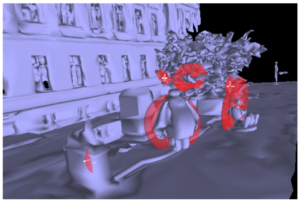
To achieve removal detection, our approach differs from the state of the art in the choice of regions of interest for 2D change detection. The reprojection method used to process the images generates regions of occlusions, as seen in
Figure 2, which are ignored in other approaches, but are the primary focus in ours. When there are inconsistencies between the mesh and the image sequence, errors occur during the reprojection process (see
Figure 3 and
Figure 4) whose location are used to detect changes.
In summary, the proposed method is comprised of five steps:
For each image of the sequence, create reprojected copies to fit the points of view of the other images.
For each point of view, render the delta maps between the corresponding sequence’s image and each accordingly reprojected image.
For each point of view, combine the delta maps into a single delta map to reduce false positives.
For each combined delta map, filter and group the pixels of detected changes into 2D areas of changes.
Match the 2D areas from one point of view to the other to infer the 3D locations and sizes of detected changes.
3.1. Image Reprojection and Occlusion Handling
In this paper, “reprojection” is not strictly used in its conventional meaning; it here amounts to back-projecting pixels onto the mesh and rendering them using another projection. This process is formalized in the next paragraphs, insisting on the impact of occlusions.
Let
and
be the projection matrices of cameras
and
. Then, a pixel
x rendered by
using
can also be back-projected to the closest 3D point
of the mesh. The back-projection function of
is called
:
Using
and
, any pixel
x from point of view
i can be associated with a pixel
from point of view
j:
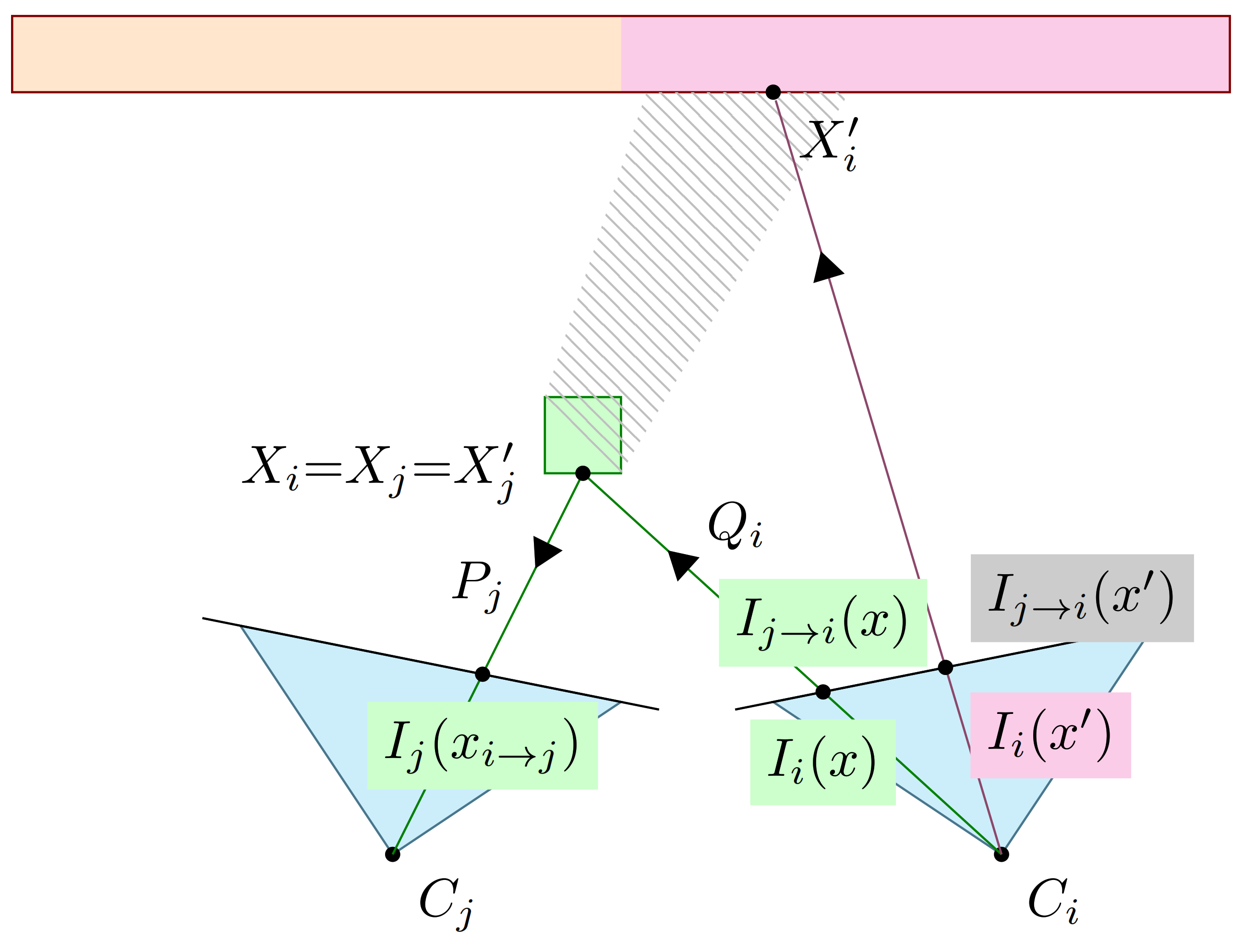
This process is illustrated in
Figure 2: Every pixel
x from point of view
i is back-projected to its corresponding
and then projected to
in the point of view
j. If performed on all the
x coordinates in
i, it can be used to assign a pixel value
to their corresponding
in
j and render a “reprojected” image
. Alternatively, the exact same transformation can be used to assign to each
x in
i a unique pixel value
and render
(see
Figure 5c) with Algorithm 1.
Using this alternative, each and every point of the “reprojected” image is given a unique value, obviating the need for a depth buffer and the necessity to interpolate any pixels that would have remained blank after the transformation. Indeed, multiple
x can reproject to the same
, but all
x reproject to some
if a corresponding 3D point can be found in the mesh.
| Algorithm 1: Base pseudo-code of our image “reprojection” process |
 |
When every pixel of the reprojected image is computed, some pixels are associated with 3D points that were occluded in the original view and, therefore, have no RGB value (see in
Figure 2). We can check for such cases during the application of the transformation. For
as defined in Equation (
2):
In Equation (
3),
and
can be different from one another, as the latter is obtained by back-projecting
using
, and is by definition the closest point to the camera. Since they are on the same axis,
not occluding
means they are equal. In contrast, in
Figure 2,
, meaning that
is occluded.
In existing methods, occluded 3D points will be discarded when computing 2D changes (see
Figure 5c). Conversely, our method systematically assigns an RGB value to these points: the one associated with the occluding point. Rendering those points with these RGB values has the effect of creating a textured shadow
, as in
Figure 4 and
Figure 5d, of the occluding points. Using Equations (
2) and (
3), we can render
with Algorithm 2.
| Algorithm 2: Pseudo-code of our “textured shadow” rendering process |
 |
3.2. Photo-Consistency in Occluded Pixels
When reprojecting, removed objects that are still present in the mesh have the effect of back-projecting the colors of the points they mask onto their surface (see in
Figure 5c, where the statue’s podium is projected onto the middle red shape) and leaving those points untextured. Rendering the regions of occlusion using Algorithm 2 avoids this back-projection effect (see in
Figure 5d where the podium is correctly placed).
More generally, the textured shadows of removed objects will be photo-consistent [
35] with the reference image, i.e., they fill holes in the warped image with accurate data (compare the yellow shadows in
Figure 5d to the reference in
Figure 5a). However, for unchanged objects, such back-projections will not be textured by occluded points, but by the object itself, and will therefore not be consistent with the reference image (see the lion statue’s shadow on the left side of
Figure 5d). Our approach consists of looking for the regions of least change between the reference image and the textured shadow images from different points of view.
The delta maps
(see in
Figure 6a) are computed using the norm 2 distance between the RGB values of each rendered pixel in the textured shadow and in the reference images [
36]. In order to account for the inaccuracies of the warping process, either in the camera pose or in the 3D mesh, the reference pixel’s color is compared to the color of all pixels in its neighborhood
in the warped image [
37]. The minimum value is chosen:
where
d is the neighborhood size and
if
is rendered.
3.3. Photo-Consistency with Multiple Points of View
As we will further detail in the following paragraphs, a single delta map per point of view will generally not contain enough information to accurately retrieve the 2D location and shape of a change. Firstly, the regions of least change computed in
Section 3.2 are located within the shadows of the foreground objects rather than in their actual position in the frame. Secondly, only the parts of a removed object that cast such shadows will be detectable, which is why using several points of view can enable the method to more closely retrieve the shape of the whole object by uncovering new parts of it with each additional view.
3.3.1. Foreground Projection
Before combining the multiple delta maps for different points of view, we first project the detected removals onto the foreground (see
Figure 6b). For any pixel
x of the delta map
, we can obtain the corresponding pixel
in the original point of view
j:
Moreover, if
is occluded, back-projecting
will return one of its occluding points
. More specifically, it will be the closest one to camera
:
which corresponds to the pixel
in point of view
i:
We adapt Equation (
3) to fit the point of view
i and avoid rendering occluded objects (such as the bench on the left side of
Figure 5b visible in
and
, but not in
):
is the closest point to
that could occlude
. Equation (
8) checks whether they are the same or not. We note that, as opposed to the reprojection process (Algorithm 2), this transformation is not reversible due to the repeated use of the back-projection, which always returns the closest point to the camera. In practice, this means that not every pixel of the foreground is assigned a value (see the white holes inside the shapes of
Figure 6b), while some pixels are given multiple values. The correct value is chosen using a depth buffer
associated with
, and the foreground-projected delta map
is then rendered using Algorithm 3.
| Algorithm 3: Pseudo-code of our foreground projection process |
 |
3.3.2. Combination of Projected Delta Maps
In
, not every pixel is assigned a value (Algorithms 2 and 3) (see the white pixels in
Figure 6b. Therefore, we can define for each
a binary mask
:
In order to uncover new parts of a potentially removed object, the combination of two projected delta maps with the same point of view involves the union of their binary masks. As for their values, the maximum per pixel of the two is chosen in order to reduce false positives. The maximum value is used to be more selective in the detection process. Foreground objects that are not removed could still share some RGB values with the background they occlude for a particular point of view (i.e., be photo-consistent), but it is unlikely they would for every point of view.
This approach is similar to the intersection process described in [
34]. There, in a single delta map, when an object is inserted into a scene, changes are detected at the correct position of the object in the reference image and at an erroneous position resulting from the projection from another point of view (see
Figure 3). Since the actual 2D location of the change is the former, the erroneous positions are removed by intersecting two different delta maps, requiring three points of view in total. However, in this previous paper, the intersection process shrinks the area of the combined mask with every new point of view instead of expanding it. This further reduces the chances of false positives, but is not practical for the study of occluded regions, which potentially do not overlap for every point of view, even after foreground projection.
Using every available point of view, we define the combined delta map
:
If x is not in any of the , then remains unassigned.
3.4. Three-Dimensional Localization of Changes
Similarly to the process described in [
34], the 3D localization relies on the segmentation of the combined delta map
into 2D regions of detected change and the matching of those regions from one point of view
i to another. From these matched regions’ locations in the images, we can infer the 3D location of the change and its spread, as detailed in the following paragraphs.
3.4.1. Segmentation by Region
The segmentation is achieved similarly to [
34]; namely, the generation of the regions’ contours using [
38] on a binarized
. Our contribution to this process is a more generalized binarization step that relies on a triangle threshold method described in [
39], rather than an arbitrary constant threshold value. The darkest pixels in
are selected as candidates for the removal detection since they describe the regions of least change in the textured shadows. Isolated pixels are then removed through erosion and the contours are generated. A final threshold on the area of the regions is used to remove the smallest changes [
34] (see
Figure 7b).
3.4.2. Region Matching
A 3D region of change that is visible for two or more points of view should have its projected 2D regions represented in several segmented delta maps. Although the 3D location of the changes could be retrieved through the use of back-projection, in practice, the segmented maps are an approximation of the 2D projected changes, and a pixel-wise depth estimation would be inaccurate. This is why we use moments [
40] to compute the centroids of each region and then the same triangulation process described in [
34].
Our method differs in the criteria used for matching the regions: Instead of computing and comparing the hue saturation value (HSV) histograms of the regions in the corresponding images, we rely on the back-projection of the centroids on the mesh. This change is necessary because of the focus on the detection of removed objects, which, by definition, are present in the mesh, but not in the images. This is a factor in the bias of detection toward inserted objects in [
34]. If the back-projected centroid of a region in
i is projected inside a region in
j (or “reprojected” from
i to
j), and vice-versa, then the two regions are matched, as in
Figure 8: The orange and blue centroids belong to matched regions, as do the red and green ones.
The triangulation step produces 3D ellipses based on the sizes and locations of the matched regions [
34]. This final output is presented in
Figure 9.
4. Experimental Evaluation and Results
The algorithm was implemented in C++11 using the source code from [
34] as a basis. Meshes and camera poses were handled using GLOW (OpenGL Object Wrapper) [
41], mathematical operations were computed with Eigen [
42], and images were processed with OpenCV [
43]. The code will be available at
https://github.com/InterDigitalInc/ (accessed on 22 January 2021).
Our method was evaluated on several scenes that presented some changes: At least one object is removed, and in some cases, some are inserted. The sequences are made up of five pictures that display the location of the removals, which are introduced by adding 3D objects to an existing accurate mesh of the scene. Conversely, insertions are simulated by removing objects from that mesh. Meshes were taken from two sources: the dataset introduced in [
34] and the ScanNet [
44] dataset (all images and receiver operating characteristic (ROC) curves from the datasets are available in the appendix), which also provide estimated camera poses for the images.
The scenes in the dataset from [
34] already showcase one or more insertions. Each mesh is already associated with five pictures that display the inserted objects. However, this dataset has some limitations: There are approximations in the meshes that can be detected as changes, and the camera distortion coefficients are not available for every camera used, which leads to inaccurate projection.
In contrast, the ScanNet dataset images are noisier, but have been corrected distortion-wise. The scenes do not contain any insertions, and all meshes are associated with a video with thousands of frames, from which we picked five with the least motion blur possible to ensure that the camera poses were accurate.
Since we compare our method with the one in [
34], the images were also chosen to showcase the location of the removed object we added to the mesh. For the sake of this comparison, we also scaled the pictures to a width of 500 px and used an area threshold of 50. Delta maps were computed using neighborhoods
of size
.
4.1. Quantitative Evaluation
In order to evaluate the change detection quality, we used the same criteria as in [
34] and [
32]: For each image point of view, we have a corresponding 2D ground truth that we compare to the results of our 3D detection. The 3D ellipses are rendered in 2D using each camera pose and numerical results are averaged across multiple points of view. The following numbers were computed for the evaluation:
IoU: area of the intersection of the ground truth and the 2D ellipse, divided by the area of their union;
coverage: area of the aforementioned intersection, divided by the area of the ground truth, i.e., true positive rate (TPR),
false positive rate: area of the intersection of the complementary ground truth and the 2D ellipse, divided by the area of the complementary ground truth.
For the scenes that contain inserted objects, we also took into account that the method described in [
34] detects changes of all natures indiscriminately. Therefore, we subtracted the shapes of the inserted objects from the image comparisons between the ground truth of removals and the 2D ellipses. Consequently, any insertion that was correctly reported by the algorithm is not be considered as a false positive for object removal detection.
4.1.1. IoU and Coverage with Automatic Thresholding
The chosen criteria favor detection that is accurate in 2D, but not necessary correctly localized in 3D, i.e., if there are several 3D regions of change accurately detected in 2D, but incorrectly matched together. Since this does not happen with our removal detection, using a 3D-based criteria could improve the performance of our method compared to the one in [
34].
In most cases, our method is the most accurate for both criteria. As shown in
Table 1, the IoU is often greater than
, but there are particularly difficult scenes where it will drop below
, while the algorithm from [
34] does not detect anything. Generally, these scenes will have a 3D mesh that is incomplete or too dissimilar from the images in areas that should have remained unchanged.
As explained in
Section 3.3.2, our approach to the combination of delta maps is based on mask union rather than intersection. This makes the detection more robust for objects nearing the edge of the frame.
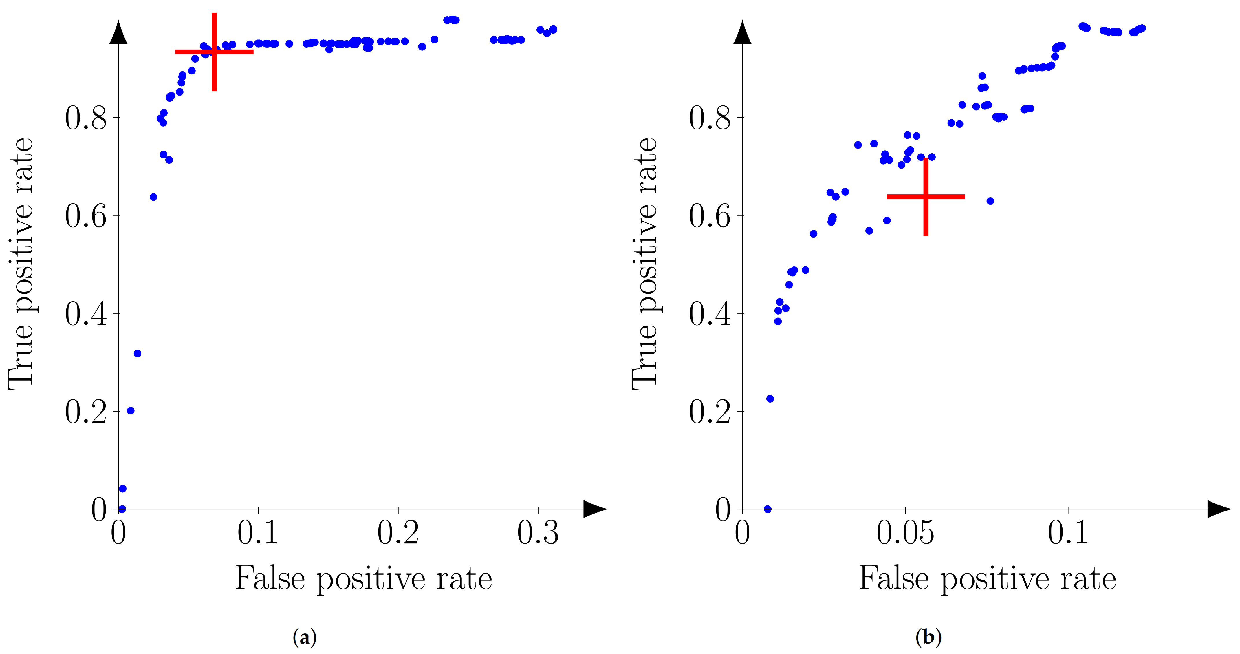
4.1.2. ROC Curves for Different Thresholds
The ROC (receiver operating characteristic) curves in
Figure 10 are used to compare the true positive rate and false positive rate of a binary operator for different discrimination thresholds [
32], which, in our case, are the value thresholds in the delta maps. The automatic threshold is highlighted on the curves to evaluate its performance, and the other threshold values are all the integers between 0 and 255. A threshold of 255 means that only the most consistent pixels of a delta map are considered (near the origin of the graphs).
We note that the false positive rate never reaches 1 in the presented curves. This is due to the fact that ellipses are only generated for objects that cast shadows during reprojection, which generally only represents a small part of any given image. The value obtained for a threshold of 0, when any pixel in the delta map’s mask is categorized as “changed” regardless of value, is the de facto maximum.
In these curves, the best results are located in the top left. The automatic threshold value is generally chosen among those ideal values, but there are instances, such as in “playground-car” (
Figure 10b), where it is at a local minimum. These discontinuities are a consequence of the thresholding by the changes’ areas and the following segmentation into 2D regions.
4.2. Computation Time
The method was run on a CPU in order to compare its speed with other similarly computationally inexpensive methods for portable devices. The execution time is in the same order as the one reported in [
34] as interactive time. The processes of generating the delta maps and triangulating the changes in 3D never take longer than a few seconds.
Of the two processes mentioned above, the former is more computationally expensive. The re-projection operations as well as difference calculations on the images are performed in a single pass on each pixel of each image. Empirically, we measured that the computation time was indeed proportional to the image size (in pixels).
The computation time of the triangulation process cannot be evaluated as reliably, since it depends on the number of 2D areas detected in the first step. However, for a constant area threshold, it will become less negligible when compared to the time of the first process, as the number of individual detected changes increases with the resolution. When the area threshold is increased in accordance with the resolution, this effect is less pronounced. The overall computation time is also tied to the number of images in the sequence.
On a virtual machine with 16 GB of RAM and four 2.60 Ghz processors, both [
34]’s method and ours process sequences of five 500 pixel-wide images in less than 3 s. For the reprojection and delta map rendering processes, we experimented with the use of shaders directly applied to the mesh instead of functions run on the depth maps derived from it. In this configuration, the execution time becomes tied to the precision of the mesh rather than the image resolution because no depth map has to be generated. When such shaders were run on an NVIDIA GeForce RTX 2060 GPU, the computation time of the aforementioned processes was reduced by up to
.
When compared to the implementation by [
34], the computation time remains low because the reprojection process, which is the most time-consuming operation, can be performed for both occluded and visible pixels in a single pass. In practice, both the algorithm from [
34] and ours can be used at the same time in order to detect both insertions and removals with more accuracy.
4.3. Discussion
Only studying regions occluded by a foreground object has a few side-effects. For instance, false positives can only be detected on objects that produce such occlusions. These false positives will only occur on the objects that are the most photo-consistent with their background (see “0001_00+dollhouse”). Moreover, any removal accurately detected in 2D will be accurately localized in 3D. This differs from insertion detection, where accurate 2D regions of change can be wrongly matched with other regions from a different change in another point of view.
In a scene, reflective surfaces might still pose a challenge instead of being detected as false positives, as in [
34]; they can make removed objects situated in their foreground difficult to detect, i.e., generate false negatives.
Change size estimation can be an issue, as the detection size is proportional to the occlusion size of the removed object (see “0000_02+statue”). If a removed object does not produce any occlusion, it will not be detected by this method. Such an object could be detected using the method from [
34] if it is far enough from its background to greatly distort its textures.
Not every image of the ScanNet dataset’s sequences is perfectly aligned with its corresponding 3D mesh (see “0005_00+bucket’). While this has not severely impacted the results of the detection in our experiments, in theory, a misalignment of an image will generate 2D false positives and negatives for its point of view. On one hand, false positives are still dealt with by using the other images of the sequence. On the other hand, false negatives can negatively impact the detection by reducing the areas of detection and lead to 3D false negatives or inaccurate size estimation. However, they occur less often, since they require that a removed object aligns with an object still present in the image.
The appendix contains further discussion of the results on a per-scene basis, as well as previews for all the scenes present in the datasets.
5. Conclusions
In this paper, we introduced a new approach for detecting the removal of objects between an outdated 3D mesh and a set of up-to-date pictures of a scene. The technique is based on the projection of the foreground of those images onto the 3D mesh, which is then observed from each other’s points of view and compared in 2D to a reference image from those points of view. The definition and study of the foreground make our approach distinctive and allow for this particular focus on object removals as opposed to changes in the scene of another nature, simplifying the process of translating the results back into the 3D world. The technique is able to perform well even in environments with uniform textures or changes of different natures while remaining as fast as the state-of-the-art methods that are meant to run on devices with low computational power.
The results could be improved by using the information contained in the mesh to estimate the 3D shape of the changes, rather than relying on standard shapes like ellipses. This could also be accomplished using a voxelization of the scene, like in other works [
18]. Once the shape estimation is more accurate, it could be used to directly alter the mesh to reflect the detected changes. With the short computing time, this process could be repeated at a high rate to retrieve cleaner results or uncover different layers of change.
With removals now specifically identified, it is possible to ignore their impact on the change detection algorithm proposed in [
34]. This improves the detection of inserted objects in scenes, and allows for the categorization of all changes according to their natures. This categorization can be expanded on by including the notion of “displacement” of an object when it is both removed and inserted into a scene.
Supplementary Materials
The following are available online at
https://www.mdpi.com/2079-9292/10/4/377/s1, Document S1: Detection of removed objects in 3D meshes using up-to-date images—Appendix; Video S2: Step 1—Image capture; Video S3: Step 2—Change detection; Video S4: Step 3—Example of application.
Author Contributions
Data curation, O.R.; formal analysis, O.R.; funding acquisition, M.F. and G.M.; investigation, O.R.; project administration, M.F. and G.M.; software, O.R.; supervision, M.F., C.B. and G.M.; validation, O.R.; visualization, O.R.; writing—original draft, O.R.; writing—review and editing, O.R., M.F., C.B. and G.M. All authors have read and agreed to the published version of the manuscript.
Funding
This research was funded by Association Nationale de la Recherche et de la Technologie (CIFRE grant).
Data Availability Statement
The code will be available at
https://github.com/InterDigitalInc/ along with instructions detailing the construction of the dataset used to evaluate the performance of the method.
Conflicts of Interest
The authors declare no conflict of interest.
Abbreviations
The following abbreviations are used in this manuscript:
| MR | mixed reality |
| LiDAR | light detection and ranging |
| RGB | red–green–blue |
| HSV | hue saturation value |
| IoU | intersection over union |
| TPR | true positive rate |
| ROC | receiver operating characteristic |
References
- Freeman, R.; Steed, A.; Zhou, B. Rapid Scene Modelling, Registration and Specification for Mixed Reality Systems. In Proceedings of the ACM Symposium on Virtual Reality Software and Technology, VRST ’05, Monterey, CA, USA, 7–9 November 2005; Association for Computing Machinery: New York, NY, USA, 2005; pp. 147–150. [Google Scholar] [CrossRef]
- Fuhrmann, A.; Hesina, G.; Faure, F.; Gervautz, M. Occlusion in Collaborative Augmented Environments; Virtual Environments, ’99; Gervautz, M., Schmalstieg, D., Hildebrand, A., Eds.; Springer: Vienna, Austria, 1999; pp. 179–190. [Google Scholar]
- Evangelidis, K.; Sylaiou, S.; Papadopoulos, T. Mergin’ Mode: Mixed Reality and Geoinformatics for Monument Demonstration. Appl. Sci. 2020, 10, 3826. [Google Scholar] [CrossRef]
- Thomas, B.; Close, B.; Donoghue, J.; Squires, J.; Bondi, P.; Piekarski, W. First Person Indoor/Outdoor Augmented Reality Application: ARQuake. Pers. Ubiquitous Comput. 2002, 6, 75–86. [Google Scholar] [CrossRef]
- Wloka, M.M.; Anderson, B.G. Resolving Occlusion in Augmented Reality. In Proceedings of the 1995 Symposium on Interactive 3D Graphics, I3D ’95, Monterey, CA, USA, 9–12 April 1995; Association for Computing Machinery: New York, NY, USA, 1995; pp. 5–12. [Google Scholar] [CrossRef]
- Simon, G. Automatic online walls detection for immediate use in AR tasks. In Proceedings of the 2006 IEEE/ACM International Symposium on Mixed and Augmented Reality, Santa Barbard, CA, USA, 22–25 October 2006; pp. 39–42. [Google Scholar]
- Bauer, J.; Klaus, A.; Karner, K.; Zach, C.; Schindler, K. MetropoGIS: A feature based city modeling system. In Proceedings of the Photogrammetric Computer Vision, ISPRS Comission III Symposium, Graz, Austria, 9–13 September 2002. [Google Scholar]
- Döllner, J.; Buchholz, H. Continuous level-of-detail modeling of buildings in 3D city models. In Proceedings of the 13th ACM International Workshop on Geographic Information Systems, Bremen, Germany, 4–5 November 2005; pp. 173–181. [Google Scholar] [CrossRef]
- Förstner, W. 3D-city models: Automatic and semiautomatic acquisition methods. In Photogrammetric Week ’99; Fritsch, D., Spiller, R., Eds.; International Society for Photogrammetry and Remote Sensing ISPRS: Stuttgart, Germany, 1999; pp. 291–303. [Google Scholar]
- Hu, J.; You, S.; Neumann, U. Approaches to large-scale urban modeling. IEEE Comput. Graph. Appl. 2003, 23, 62–69. [Google Scholar]
- Ribarsky, W.; Wasilewski, T.; Faust, N. From urban terrain models to visible cities. Comput. Graph. Appl. IEEE 2002, 22, 10–15. [Google Scholar] [CrossRef]
- Denis, E.; Baillard, C. Refining existing 3D building models with terrestrial laser points acquired from a mobile mapping vehicule. Int. Arch. Photogramm. Remote Sens. Spat. Inf. Sci. 2010, 39, 195–200. [Google Scholar]
- Izadi, S.; Kim, D.; Hilliges, O.; Molyneaux, D.; Newcombe, R.; Kohli, P.; Shotton, J.; Hodges, S.; Freeman, D.; Davison, A.; et al. KinectFusion: Real-time 3D Reconstruction and Interaction Using a Moving Depth Camera. In Proceedings of the 24th Annual ACM Symposium on User Interface Software and Technology, UIST ’11, Santa Barbara, CA, USA, 16–19 October 2011; pp. 559–568. [Google Scholar]
- Sadeghi, F.; Arefi, H.; Fallah, A.; Hahn, M. 3D Building façade reconstruction using handheld laser scanning data. ISPRS Int. Arch. Photogramm. Remote Sens. Spat. Inf. Sci. 2015, XL-1/W5, 625–630. [Google Scholar] [CrossRef]
- Park, D.H.; Darrell, T.; Rohrbach, A. Robust Change Captioning. In Proceedings of the 2019 IEEE/CVF International Conference on Computer Vision, ICCV 2019, Seoul, Korea, 27 October–2 November 2019; pp. 4623–4632. [Google Scholar] [CrossRef]
- Fuse, T.; Yokozawa, N. Development of a Change Detection Method with Low-Performance Point Cloud Data for Updating Three-Dimensional Road Maps. ISPRS Int. J. Geo-Inf. 2017, 6, 398. [Google Scholar] [CrossRef]
- Vaiapury, K.; Purushothaman, B.; Pal, A.; Agarwal, S. Can We Speed up 3D Scanning? In A Cognitive and Geometric Analysis. In Proceedings of the 2017 IEEE International Conference on Computer Vision Workshops, ICCV Workshops 2017, Venice, Italy, 22–29 October 2017; IEEE Computer Society: New York, NY, USA, 2017; pp. 2690–2696. [Google Scholar] [CrossRef]
- Katsura, U.; Matsumoto, K.; Kawamura, A.; Ishigami, T.; Okada, T.; Kurazume, R. Spatial change detection using voxel classification by normal distributions transform. In Proceedings of the International Conference on Robotics and Automation, ICRA 2019, Montreal, QC, Canada, 20–24 May 2019; IEEE: New York, NY, USA, 2019; pp. 2953–2959. [Google Scholar] [CrossRef]
- Palma, G.; Cignoni, P.; Boubekeur, T.; Scopigno, R. Detection of Geometric Temporal Changes in Point Clouds. Comput. Graph. Forum 2016, 35, 33–45. [Google Scholar] [CrossRef]
- Schauer, J.; Nüchter, A. Removing non-static objects from 3D laser scan data. Isprs J. Photogramm. Remote Sens. 2018, 143, 15–38. [Google Scholar] [CrossRef]
- Postica, G.; Romanoni, A.; Matteucci, M. Robust moving objects detection in lidar data exploiting visual cues. In Proceedings of the 2016 IEEE/RSJ International Conference on Intelligent Robots and Systems, IROS 2016, Daejeon, Korea, 9–14 October 2016; IEEE: New York, NY, USA, 2016; pp. 1093–1098. [Google Scholar] [CrossRef]
- Caye Daudt, R.; Le Saux, B.; Boulch, A. Fully Convolutional Siamese Networks for Change Detection. In Proceedings of the IEEE International Conference on Image Processing (ICIP), Athens, Greece, 7–10 October 2018. [Google Scholar]
- Chen, J.; Yuan, Z.; Peng, J.; Chen, L.; Huang, H.; Zhu, J.; Lin, T.; Li, H. DASNet: Dual attentive fully convolutional siamese networks for change detection of high resolution satellite images. CoRR 2020. [Google Scholar] [CrossRef]
- Guo, E.; Fu, X.; Zhu, J.; Deng, M.; Liu, Y.; Zhu, Q.; Li, H. Learning to Measure Change: Fully Convolutional Siamese Metric Networks for Scene Change Detection. arXiv 2018, arXiv:1810.09111. [Google Scholar]
- Varghese, A.; Gubbi, J.; Ramaswamy, A.; Balamuralidhar, P. ChangeNet: A Deep Learning Architecture for Visual Change Detection. In Proceedings of the Computer Vision—ECCV 2018 Workshops, Munich, Germany, 8–14 September 2018; Lecture Notes in Computer Science, Part IIv. Leal-Taixé, L., Roth, S., Eds.; Springer: Berlin/Heidelberg, Germany, 2018; Volume 11130, pp. 129–145. [Google Scholar] [CrossRef]
- Blakeslee, B.M. LambdaNet: A Novel Architecture for Unstructured Change Detection. Master’s Thesis, Rochester Institute of Technology, Rochester, NY, USA, 2019. [Google Scholar]
- Cheng, W.; Zhang, Y.; Lei, X.; Yang, W.; Xia, G. Semantic Change Pattern Analysis. arXiv 2020, arXiv:2003.03492. [Google Scholar]
- Daudt, R.C.; Saux, B.L.; Boulch, A.; Gousseau, Y. Multitask learning for large-scale semantic change detection. Comput. Vis. Image Underst. 2019, 187. [Google Scholar] [CrossRef]
- Gressin, A.; Vincent, N.; Mallet, C.; Paparoditis, N. Semantic Approach in Image Change Detection. In Proceedings of the Advanced Concepts for Intelligent Vision Systems—15th International Conference, ACIVS 2013, Poznań, Poland, 28–31 October 2013; Blanc-Talon, J., Kasinski, A.J., Philips, W., Popescu, D.C., Scheunders, P., Eds.; Lecture Notes in Computer Science. Springer: Berlin/Heidelberg, Germany, 2013; Volume 8192, pp. 450–459. [Google Scholar] [CrossRef]
- de Jong, K.L.; Bosman, A.S. Unsupervised Change Detection in Satellite Images Using Convolutional Neural Networks. In Proceedings of the International Joint Conference on Neural Networks, Budapest, Hungary, 14–19 July 2019; IEEE: New York, NY, USA, 2019; pp. 1–8. [Google Scholar] [CrossRef]
- Kataoka, H.; Shirakabe, S.; Miyashita, Y.; Nakamura, A.; Iwata, K.; Satoh, Y. Semantic Change Detection with Hypermaps. arXiv 2016, arXiv:1604.07513. [Google Scholar]
- Taneja, A.; Ballan, L.; Pollefeys, M. Image based detection of geometric changes in urban environments. In Proceedings of the IEEE International Conference on Computer Vision, ICCV 2011, Barcelona, Spain, 6–13 November 2011; Metaxas, D.N., Quan, L., Sanfeliu, A., Gool, L.V., Eds.; IEEE Computer Society: New York, NY, USA, 2011; pp. 2336–2343. [Google Scholar] [CrossRef]
- Ulusoy, A.; Mundy, J. Image-Based 4-d Reconstruction Using 3-d Change Detection. In Proceedings of the European Conference on Computer Vision, Zurich, Switzerland, 6–12 September 2014; Volume 8691. [Google Scholar] [CrossRef]
- Palazzolo, E.; Stachniss, C. Fast Image-Based Geometric Change Detection Given a 3D Model. In Proceedings of the IEEE International Conference on Robotics & Automation (ICRA), Brisbane, Australia, 21–25 May 2018. [Google Scholar]
- Kutulakos, K.N.; Seitz, S.M. A Theory of Shape by Space Carving. Int. J. Comput. Vis. 2000, 38, 199–218. [Google Scholar] [CrossRef]
- Gevers, T.; Gijsenij, A.; van de Weijer, J.; Geusebroek, J.M. Color in Computer Vision: Fundamentals and Applications, 1st ed.; Wiley Publishing: Hoboken, NJ, USA, 2012. [Google Scholar] [CrossRef]
- Taneja, A.; Ballan, L.; Pollefeys, M. Modeling Dynamic Scenes Recorded with Freely Moving Cameras. In Proceedings of the Computer Vision—ACCV 2010—10th Asian Conference on Computer Vision, Queenstown, New Zealand, 8–12 November 2010; Kimmel, R., Klette, R., Sugimoto, A., Eds.; Lecture Notes in Computer Science; Revised Selected Papers; Part III. Springer: Berlin/Heidelberg, Germany, 2010; Volume 6494, pp. 613–626. [Google Scholar] [CrossRef]
- Suzuki, S.; Abe, K. Topological structural analysis of digitized binary images by border following. Comput. Vis. Graph. Image Process. 1985, 30, 32–46. [Google Scholar] [CrossRef]
- Zack, G.W.; Rogers, W.E.; Latt, S.A. Automatic measurement of sister chromatid exchange frequency. J. Histochem. Cytochem. 1977, 25, 741–753. [Google Scholar] [CrossRef] [PubMed]
- Hu, M.K. Visual pattern recognition by moment invariants. IRE Trans. Inf. Theory 1962, 8, 179–187. [Google Scholar]
- GLOW (OpenGL Object Wrapper). Available online: https://github.com/jbehley/glow (accessed on 5 January 2021).
- Guennebaud, G.; Jacob, B. Eigen v3. 2010. Available online: http://eigen.tuxfamily.org (accessed on 1 February 2021).
- Bradski, G.; The OpenCV Library. Dr. Dobb’s J. Softw. Tools 2008. Available online: https://opencv.org (accessed on 1 February 2021).
- Dai, A.; Chang, A.X.; Savva, M.; Halber, M.; Funkhouser, T.; Nießner, M. ScanNet: Richly-annotated 3D Reconstructions of Indoor Scenes. In Proceedings of the Computer Vision and Pattern Recognition (CVPR), Honolulu, HI, USA, 21–26 July 2017. [Google Scholar]
| Publisher’s Note: MDPI stays neutral with regard to jurisdictional claims in published maps and institutional affiliations. |
© 2021 by the authors. Licensee MDPI, Basel, Switzerland. This article is an open access article distributed under the terms and conditions of the Creative Commons Attribution (CC BY) license (http://creativecommons.org/licenses/by/4.0/).


