Abstract
In personalized healthcare, an ecosystem for the manipulation of reliable and safe private data should be orchestrated. This paper describes an approach for the generation of synthetic electrocardiograms (ECGs) based on Generative Adversarial Networks (GANs) with the objective of anonymizing users’ information for privacy issues. This is intended to create valuable data that can be used both in educational and research areas, while avoiding the risk of a sensitive data leakage. As GANs are mainly exploited on images and video frames, we are proposing general raw data processing after transformation into an image, so it can be managed through a GAN, then decoded back to the original data domain. The feasibility of our transformation and processing hypothesis is primarily demonstrated. Next, from the proposed procedure, main drawbacks for each step in the procedure are addressed for the particular case of ECGs. Hence, a novel research pathway on health data anonymization using GANs is opened and further straightforward developments are expected.
1. Introduction
In recent years there has been a huge proliferation of solutions that store and process personal health data and infer knowledge, from mobile health apps to smart wearable sensors [1]. In Reference [2], a proposal is introduced to orchestrate an ecosystem of manipulation of reliable and safe data, applied to the field of health, proposing the creation of digital twins for personalized healthcare [3].
One of the elements to be considered in health-related projects is data privacy for ethical issues. Sources of medical data in health services are causing important concerns, the main one being privacy and legal issues when sharing and reporting health information of patients. However, an accurate diagnosis depends on the quantity and quality of the information about a patient, as well as extensive medical knowledge. In this context, anonymization arises as a tool to mitigate the risks of obtaining and massively processing personal data [4]. We propose GAN-based anonymization [5] of private health data, so a seedbed would be obtained from the training data that allow not only to capture information from the original data, but to generate new information with a similar behaviour.
Generative Adversarial Network (GAN) algorithms have arisen in 2014 [6] and, since then, have been highlighted as potential alternatives for data augmentation [7] and missing data problems [8], among other applications, due to their outstanding capabilities on generating realistic data instances, mostly images. Following these applications, a question raised about the feasibility of using GAN systems to generate synthetic data, not necessarily images, that imitates the attributes of a private health database. If possible, this generated machine would be a very useful tool as it is enabling unlimited similar-to-the-original data without compromising the privacy of the original elements. The applications of this tool could range from educational purposes to scientific simulations and investigations, as sensitive data from any field could be available without a risk of private data leakage.
This article is subsuming, extending and completing recent work in [9,10]. It starts by elaborating on the very first approach of using GANs for the generation of synthetic data in the health domain avoiding as far as possible original images as samples, but usual raw data. In Reference [9], it was demonstrated how GANs can be used for an anonymization process on personal biometric image data; in [10], the original result was extended to general static (clinical records) and dynamic (time-series) databases. Next, we are extending the original approach on electrocardiograms (ECGs), which are 15-dimensions time signals usually interpreted by medical staff in a graphic form. We focus on several concerns emerging from the original anonymization procedure about data transformation in images, usual deep learning drawbacks (mode collapse, diminished gradient) and evaluation measures (convergence, quality). Their analysis and results complete the current study and open new lines of research in domains as soft-sensors, deep learning and metrics. Hence, specific objectives for this work include the study of (i) pre-processing datasets for its correct manipulation; (ii) training GAN systems, and (iii) analyze the obtained results under several metrics and define further steps in the research.
This paper is organized as follows. In the next section, a brief introduction to Generative Adversarial Networks is provided. Next, the problem setup is settled and the original GAN-based anonymization procedure derived from results in [9,10] is shortly introduced. Several main concerns and drawbacks related with the different steps in the original anonymization process are developed in an experimental part for the particular case of an ECG database. Finally, a discussion about main results follows and further research issues are listed.
2. Generative Adversarial Networks
Generative Adversarial Networks (GANs) [6] are systems based on a min-max strategy where two algorithms are confronted: one algorithm generates data (the generator) and the other discriminates between synthetic and real data (the discriminator). The generator’s objective is to maximize the discriminator error while the discriminator wants to minimize it. This is an iterative process that ends when the discriminator fails to recognise generated synthetic data, approximating the baseline error. In order to generate a synthetic image, a source of “creativity” coming from a random noise vector (seed) is needed. Moreover, a database of real images is needed to be able to discriminate between real and synthetic images, so that the discriminator model can send to the generator model what is doing wrong. Hence, the objective function of the complete network is the following:
This expression represents the value (V) of our current GAN system, which is a function of both, the discriminator D and the generator G, where
- represents the distribution of real data.
- represents the distribution of noise, usually a Gaussian distribution, from which we can generate a synthetic image.
- x and z represent the samples from each corresponding space.
- and represent the expected log likelihood from the different outputs of both real and generated images. We will be referring to the calculated error as loss.
- D function outputs a real number ranged between 0 and 1 representing the probability for data being real (1) or synthetic (0). On the other hand, G function outputs a generated sample or instance.
The goal is to maximize the discriminator (D) loss and minimize the generator (G) loss. The sum of expected log likelihood for real (x) and generated (z) data is the Value V for the current GAN architecture. Maximizing the resulting values leads to optimization of the discriminator parameters such that it learns to correctly identify both real and synthetic data. In order to train the generator and the discriminator, errors on their outputs are propagated back into the models.
3. Background
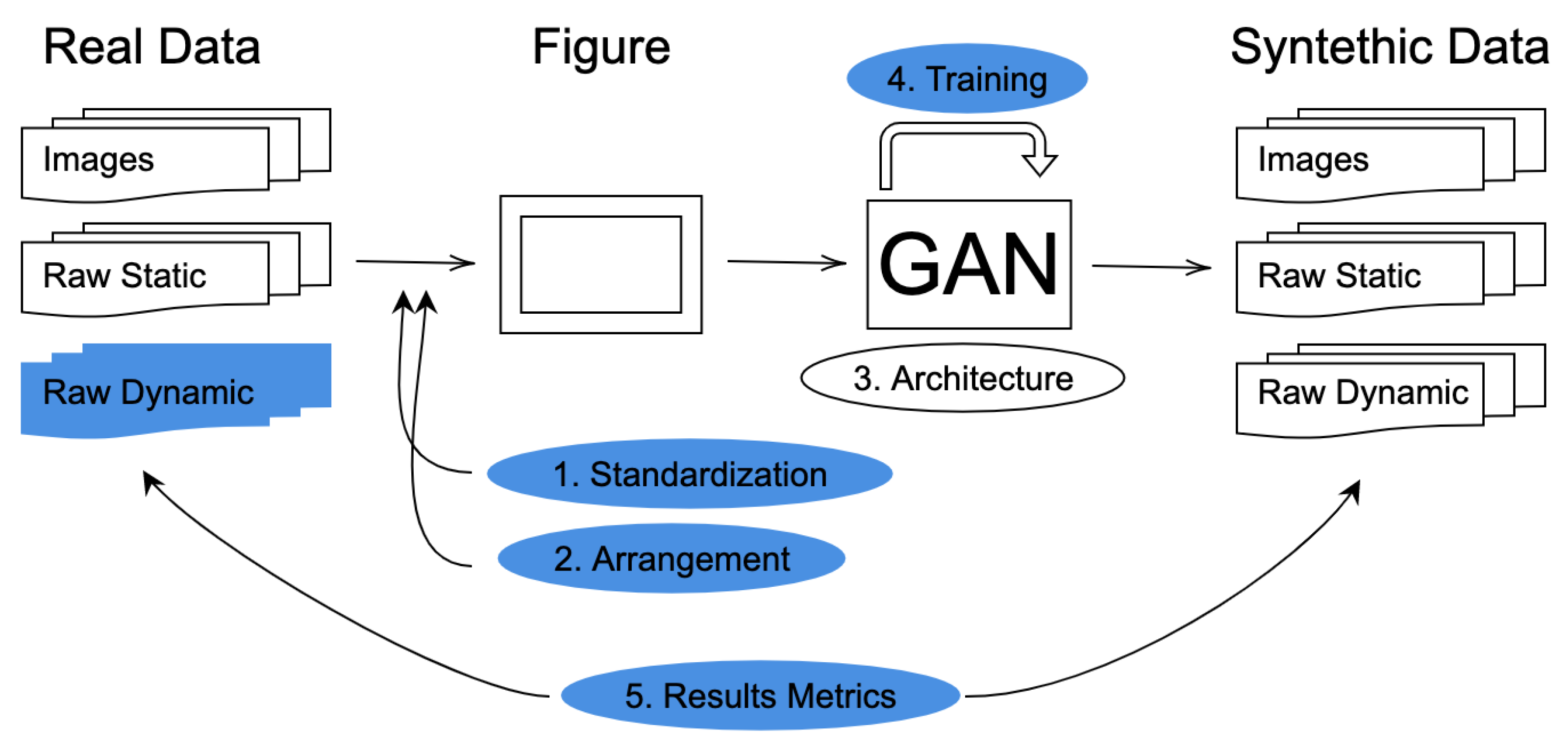
In this section the problem setup is defined and starting results in [9,10] are shortly introduced. As a first result, in this work a novel five steps procedure is defined for GAN-based anonymization of general data. As shown in Figure 1, we are concerned in this section on the white blocks, that is, to check the general problem about anonymization of health data on both, images and raw static data. In the next section the blue blocks, that is raw dynamic data in the form of ECGs and four out of five steps in the process formulation will be analyzed.
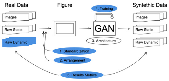
Figure 1.
Diagram with the proposed procedure and the working steps.
3.1. Problem Definition
The general environment where our anomymization system is working corresponds to an ecosystem of manipulation of reliable and safe data, applied to the field of health, for personalized healthcare [2]. Hence, the main objective is the use of Generative Adversarial Networks on sensitive health data information allowing both, anonymizing data in the form of a synthetic dataset and generating synthetic patients that health professionals can use for study.
For experimentation, specific generator and discriminator models for each database, both Fully Connected Network (FCN) with linear transfer function and Convolutional Neural Network (CNN), are implemented in the form of standard architectures (see step ‘3. Architecture’ in Figure 1).
In order to check the hypothesis of generating usable anonymized personal health data, some databases are selected. The main features under consideration are the number of samples and the available information about data. The analysed databases can be organised in two different groups: image directories and raw data directories. As a first approach, GAN anonymization was primarily focused in [2,9] on image directories, which is the most common usage. This way, it was possible to focus entirely on the hypothesis: Can (image) data be feed into a GAN system in order to yield good results on anonymization for personal data?
3.2. Hypothesis Checking on Image Directories
The Fingerprints database from ChaLearn (http://chalearnlap.cvc.uab.es/dataset/32/description/ (accessed on 10 November 2020)) with 75,600 available samples, and Iris, a database with 2224 instances of left-and-right iris images [11] collected from the students and staff at IIT Delhi, India are considered. On the whole, results in [9] show that image-like personal data anonymization through Generative Adversarial Networks is feasible, as it can be checked in Figure 2 and Figure 3. On the objectives side, it is surprising to observe the ease of conversion from images to data for the GAN system and the results obtained in a small amount of time, both for fully connected and convolutional models.
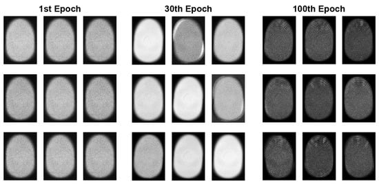
Figure 2.
Generated fingerprint images samples through 100 epoch training with an FCN model.

Figure 3.
Generated iris images samples through 200 epoch training with a CNN model.
3.3. Hypothesis Checking on Raw Data Directories
The second type of databases with general raw data generation is the one considered in [10] as a generalization step for our hypothesis checking. The Thyroid database and the Cardiogram database are considered. The Thyroid database from KEEL (https://sci2s.ugr.es/keel/dataset.php?cod=67 (accessed on 10 November 2020)) contains 7200 instances of user features that are relevant for thyroid illnesses detection. All its variables are static, meaning that for each patient there is only one value per feature without contemplate its evolution. In contrast, the Cardiogram database from Physionet (https://physionet.org/physiobank/database/ptbdb/ (accessed on 10 November 2020)) is a time series database showing the evolution of its variables through time. The main objective of the usage of this database is to simulate one of the ECG time series for a specific range of time.
Experimentation in the generation of synthetic data using GANs moves its focus from images domain to general raw data generation. This movement is not trivial, however. Raw data, unlike images, can have many different dimensions and contain values within many different ranges. Images, on the other side, are mainly represented in a range value of 0 to 255 for every pixel with a limited number of dimensions, depending whether it is grayscale, RGB, RGB-D.
Hence, in order to use the same tools as for image samples, it is proposed to uniform data and represent them in a visual way to the GAN system. This pre-processing phase is divided in two steps (see in Figure 1):
- Data Standardization: Bringing all features of the dataset to the same range value, which is from 0 to 255, and trimming all samples to same amount of values if needed.
- Data Arrangement: Configuring the layout of the data, meaning how features are placed in a shaped image, usually a square one.
A domestic parallelism of this pre-processing process could be how humans visualize data in order to understand it themselves better and quicker, ECGs being a very useful example. Feeding the original data to the GAN system in the ‘correct’ visual way could be as important as representing an electrocardiogram data to a doctor in a proper—and visual—way.
3.3.1. Data Standardization
All units are standardized to a common range to unify the weight of each variable range. The general feature scaling or normalization would be
For the Thyroid database, a is set to 1. In this form, continuous features are ranged from 1 to 255, which is the usual range for image files. The value 0 is excluded from the range so that it can be used exclusively as a NULL value. When no NULL value should be considered, as it is the case for the Cardiogram database, the normalization formula could be simplified by setting .
3.3.2. Data Arrangement
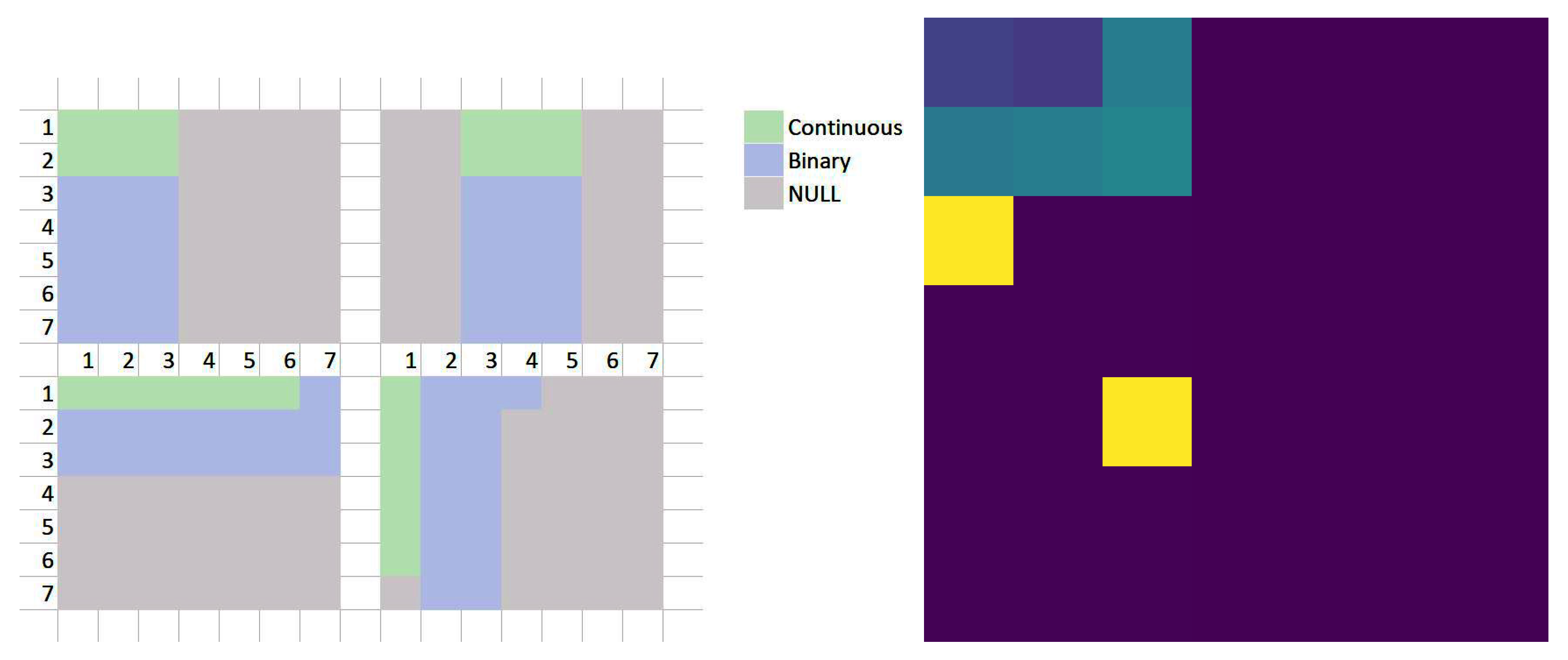
Now we can proceed to the arrangement of normalized data in an image format. Taking into account the two types of features—binary and continuous—in the Thyroid database and their number—6 and 15 respectively—many arrangements can be performed in a grid. In Figure 4 (left) some of them are displayed. The arrangement of all features is in the shape of a square area to avoid further complications whether models such as CNN are used. The selected arrangement is the first one (left, top scheme). In Figure 4, (right), there is an example of real thyroid sample turned into image. For the NULL area, all values are set to 0.

Figure 4.
(Left) Possible Thyroid’s features arrangements. (Right) Sample from the Thyroid’s database converted into an image.
Unlike the static data in Thyroid database, for the Cardiogram database the number of features is not the same for all samples—as not all patients recordings have the same length. As a solution, by trimming each user sample into equal-sized features pieces, samples have all the same amount of features and its number is greater. Size is a compromise between enough duration length and amount of total samples. In this case, patient recording is trimmed into blocks of 2025 features—removing the tail if needed—so squared images () are generated, preferred when dealing with some models such as CNNs. The number of samples goes from 549 to 28,902 while maintaining around 2 seconds of recording in each sample, which represent between two and three heart beats most of the time.
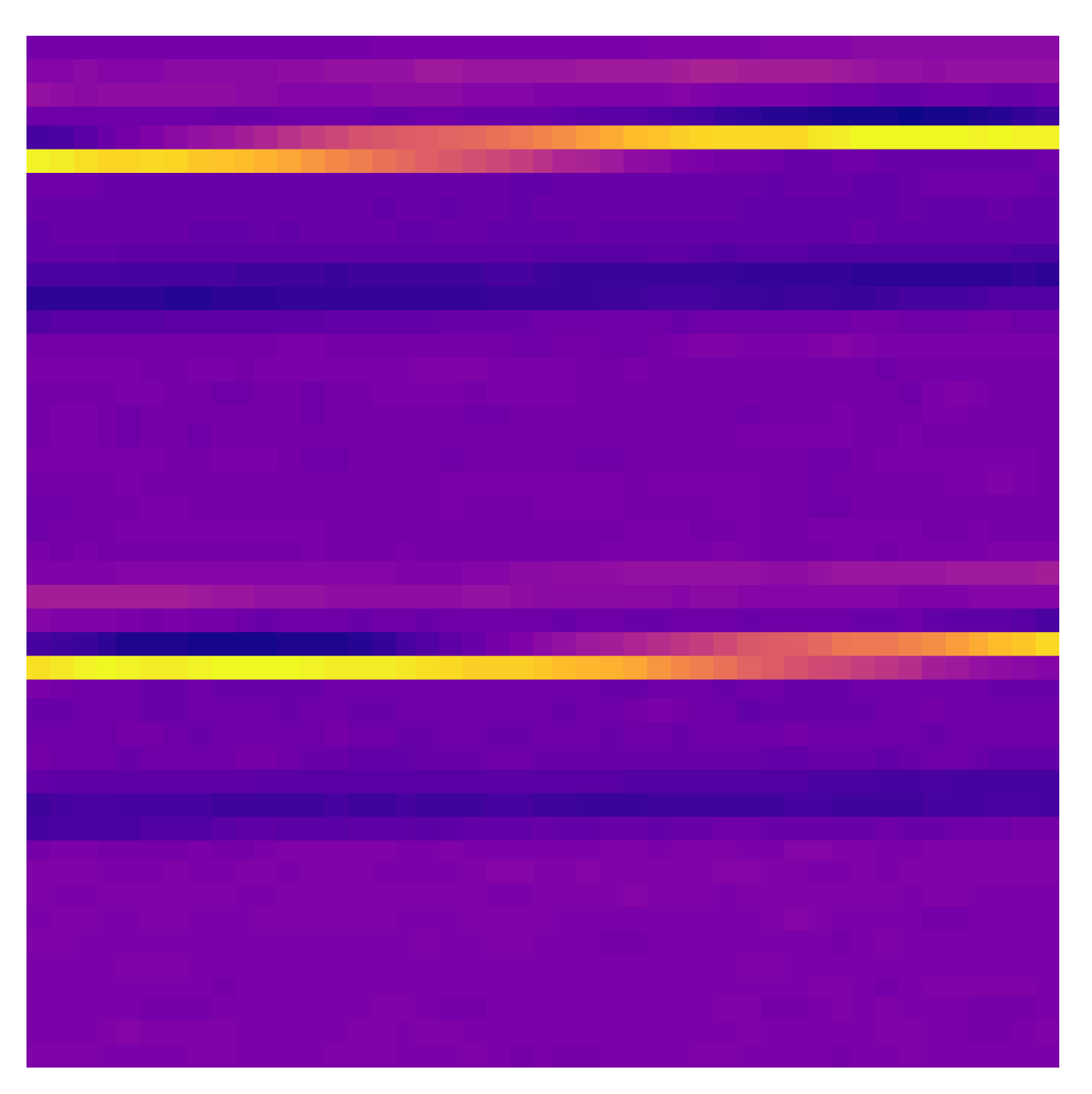
All the square area available for data to image transformation can be filled up with values of the feature. Now, many configurations are possible to determine the path that follow consecutive values in the image. Initially, it has been decided to follow a “Z” movement from left to right, then up to down. In Figure 5 there is an example for the feature signal ‘i’ turned into image with the chosen arrangement.

Figure 5.
Original sample from the first signal ‘i’ of an electrocardiogram processed into an image.
3.3.3. Model, Training and Results
Thyroid Database
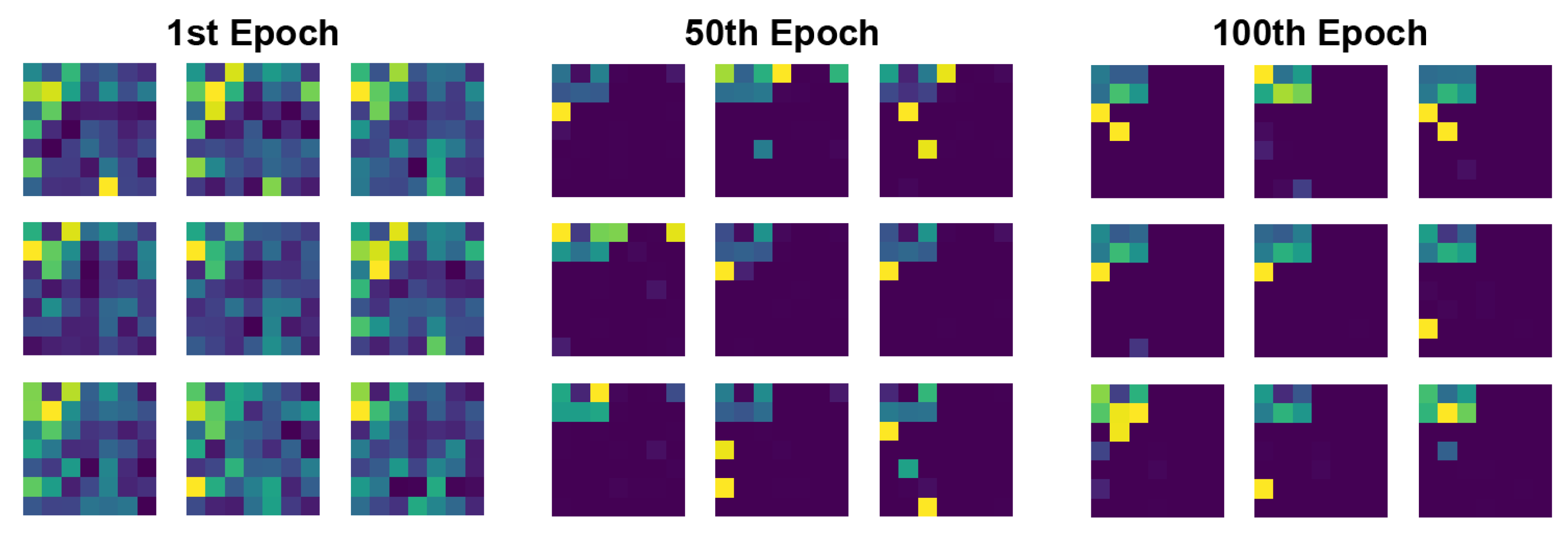
For this case the Thyroid images are fed into a Fully Connected Network (FCN) with linear activation functions. Training lasts for 100 epochs and batch size is of 20 images. Regarding FCN layers, just one 64-nodes hidden layer is considered for both the discriminator and the generator. The noise vector for the generator is sized five. After training, the generator overtakes the discriminator from the beginning, that is a diminished gradient problem [12] on the discriminator side that is causing it an inability to improve because the generator is too strong. In Figure 6, it is observed how values on the binary zone (bottom left) get contrasted values—around 1 or around 255—between epoch 1 and 50, but there are yet values on the NULL side (right side). Finally, on epoch 100 this problem is solved, all values of the NULL side being 0.
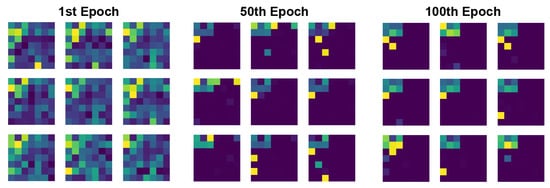
Figure 6.
Generated Thyroid images samples through 100 epochs training with a FCN model.
Next, in order to understand whether synthetic generated data is following the same distributions as the original, 6330 data samples are generated and compared to the original ones. Next, image files are converted back into numeric data and all continuous features data—both original one and generated—are visualized through box-plots [10]. In all cases, the generated samples are positioned inside the ranges of the ground truth values for all continuous features. However, the dispersion of the values is a bit different, medians does not matching Q1 and Q3 percentiles. On the side of binary variables, it has been observed that, for the same amount of samples of synthetic and real data, the total amount of positive and negative values in all features is similar between both groups.
Cardiogram Database
The second database to be imitated is the Cardiogram database from Physionet. This database contains records of 15 different signals from patient’s electrical impulses from the heart for a certain amount of time. The main objective using a GAN on this repository is to generate new anonymous cardiograms samples that look similar to the original ones. Specifically, in this case it is simulated a single signal from the 15 available, signal ‘i’. Same as on static data, in the data arrangement step data should be translated into an image format. This way it would be possible to insert all patients information to the GAN system and then receive the generated patient samples accordingly.
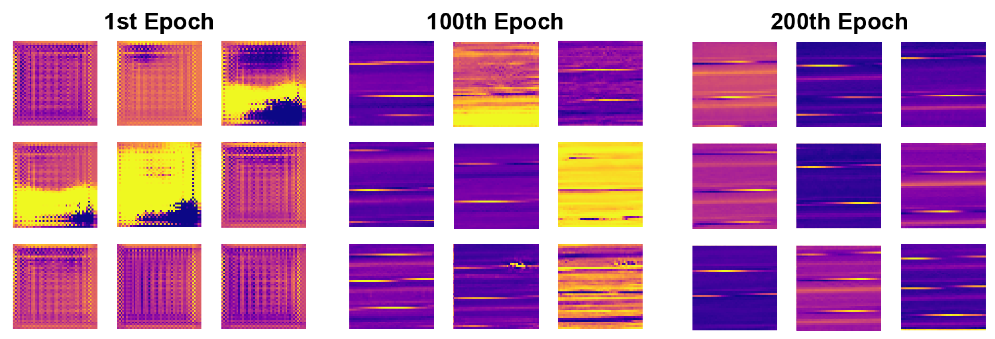
For the Cardiogram database there are 28,902 samples available. A CNN model have been configured: GAN is trained for 200 epochs with a batch size of 30. The CNN structure endows three hidden layers with 64 nodes, 128 nodes and 256 nodes, respectively. The noise vector is sized 100. As shown in Figure 7, after a few epochs, output images contain some patterns similar to the ones on ground truth samples. On the 200th epoch, main dissimilarities are gone.
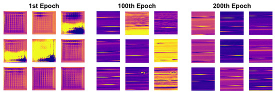
Figure 7.
Generated Cardiogram images samples through 200 epoch training with a CNN model.
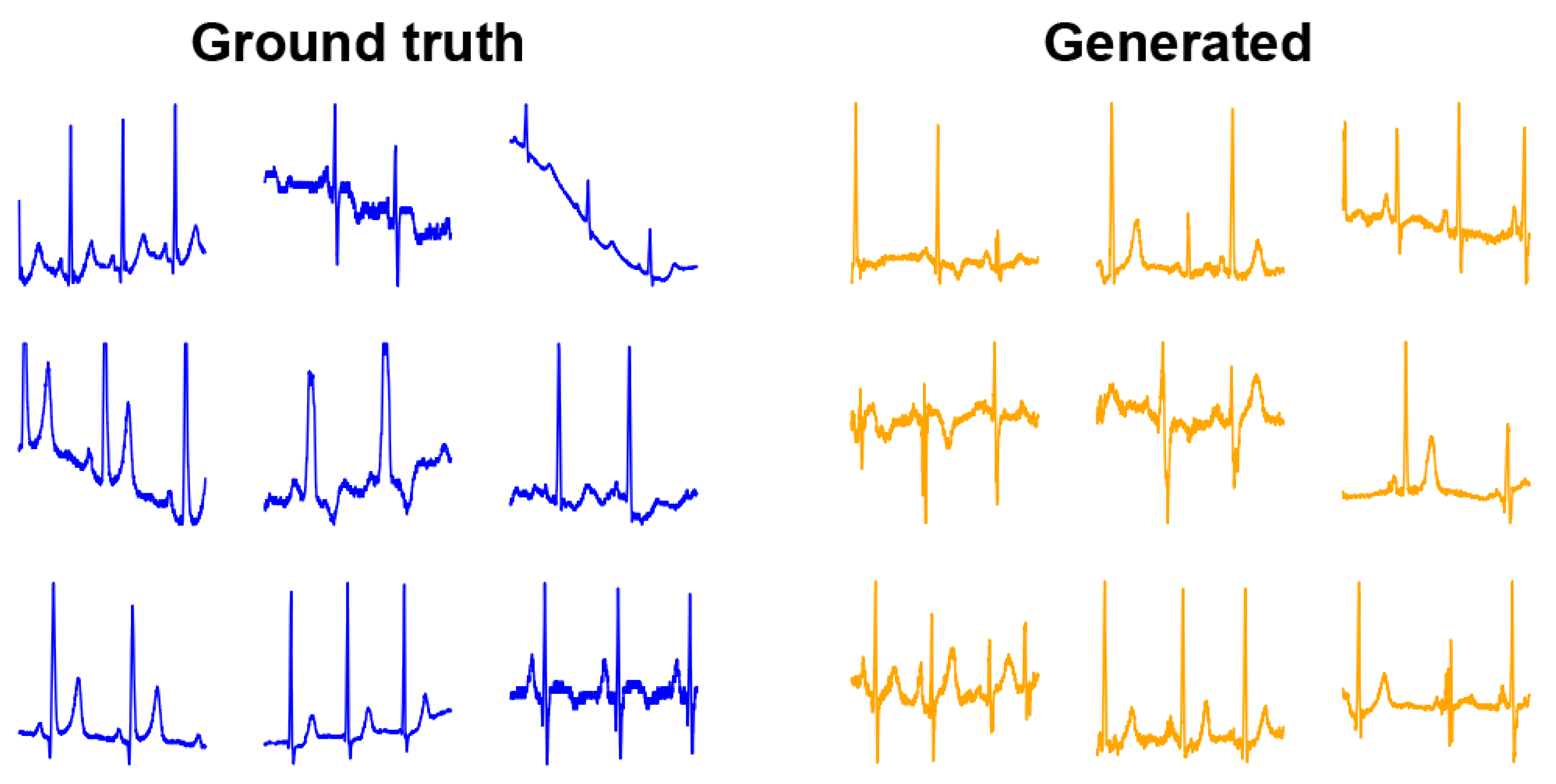
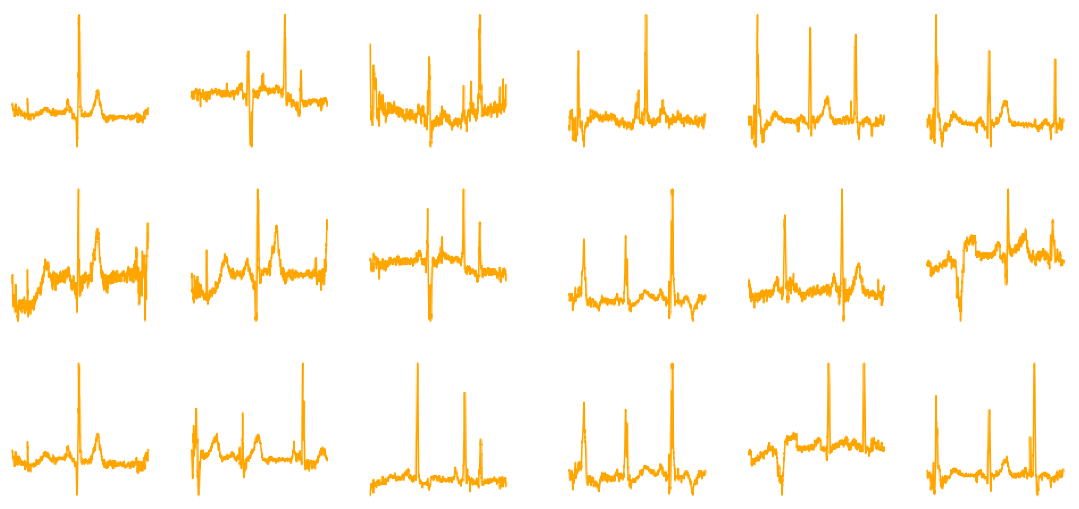
Since results are not static data, instead of analyzing the distribution of the studied feature, output data is visually compared to the original one—just how a doctor would do for this kind of information. A random sub-group of real and synthetic cardiogram data can be observed in Figure 8. It is important to highlight that current evaluation is purely based on the visual differences between synthetic and real data and the consultant of a doctor would be required. It is obvious that further research on evaluation metrics on GAN-based image solutions is needed.

Figure 8.
Ground truth Cardiogram signals vs. generated time series from samples through 200 epoch training with a CNN model.
By comparing both groups, the generated cardiograms have quite equidistant heart pulses just as the real data does. Overall patterns are very similar, with a constant base slope during all the time range. Regarding differences, there are mainly two elements. There is a clear difference on spike lengths. Ground truth heart pulses have consistently the same length, however this consistency is not solid on the generated side. On the other side, the spike pattern within the same patient seems to be always the same but on the generated group patters have slightly variations through the sample.
4. Synthetic ECGs Generated Using GANs
It has been checked in the previous section by summing-up the work developed in [9,10] that it is possible to feed a GAN system with general health data in order to yield good results on anonymization for personal data. The steps for the proposed procedure are:
- Data standardization.
- Data arrangement into an image.
- Determine GANs architecture.
- Deal with usual deep learning training concerns.
- Select appropriated results metrics.
Working on these different steps, the original solution from precedent references will be improved (blue blocks in Figure 1). The Cardiogram dataset of ECGs from Physionet has been chosen because it is a multidimensional time-series with dual raw/image nature. The National Metrology Institute of Germany has provided this compilation of digitized ECGs for research, algorithmic benchmarking or teaching purposes to the users of PhysioNet. The ECGs were collected from healthy volunteers and patients with different heart diseases by Professor Michael Oeff, M.D., at the Department of Cardiology of University Clinic Benjamin Franklin in Berlin, Germany. Each record includes 15 simultaneously measured signals: the conventional 12 lead placements (i, ii, iii, avr, avl, avf, v1, v2, v3, v4, v5, v6) together with the three Frank lead ECGs (vx, vy, vz). Each signal is digitized at 1000 samples per second, with 16 bit resolution over a range of ±16.384 mV. Available samples are 549, expandable by splitting each sample into multiple segments.
The objective in this main experimental section is to analyse which features can be improved from the original GAN-based cardio model and check valid solutions. Different techniques will be explored with the objective of achieving better results, not only in the quality of the samples but also on the stability during the GAN training. Furthermore, new GAN models will be developed. Taking into consideration these aspects to be improved, several studies are proposed exploring the GAN-based anonymization original solution:
- A new data standardization proposal.
- Straightforward new time series arrangements.
- Data arrangement in the form of RGB images: several channels at the same time.
- Introducing the concept of label smoothing.
- ACGAN architecture: using a GAN structure for classification.
- Introducing evaluation measures.
4.1. Adapted Range Data Standardization
When an exploration of the values for the electrocardiogram samples is performed, the description of the data shown that 25% and 75% quantiles values are far away from max and min values. Hence, 1% and 99% quantiles are chosen to be the bounds for the normalization, consisting of a linear regression between 0 and 255, which is the usual range for image files. Values beyond bounds are saturated. In this way, only 4% of the samples have at least one of the values outside these bounds.
Next, the histogram in Figure 9 for each signal shows that the range can be reduced from 4 (between 2 and −2) to 2.5, which will cover almost all samples. A smaller range makes the samples to have more precise and continuous standardized values.
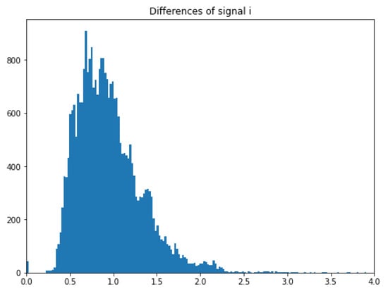
Figure 9.
Histogram for the signal ‘i’ in the ECG.
Furthermore, instead of having a fixed range, it is modified into an adapted range starting from the lowest value of the normalized sample. The resultant normalization formula is:
with since no NULL values are present, where is the minimum value into the chunk sized 2025 of the complete electrocardiogram signal. By applying these two modifications at the same time, a better-defined shape of the signals is obtained in the regions that are not the peaks.
4.2. A First Simple Data Arrangement Modification
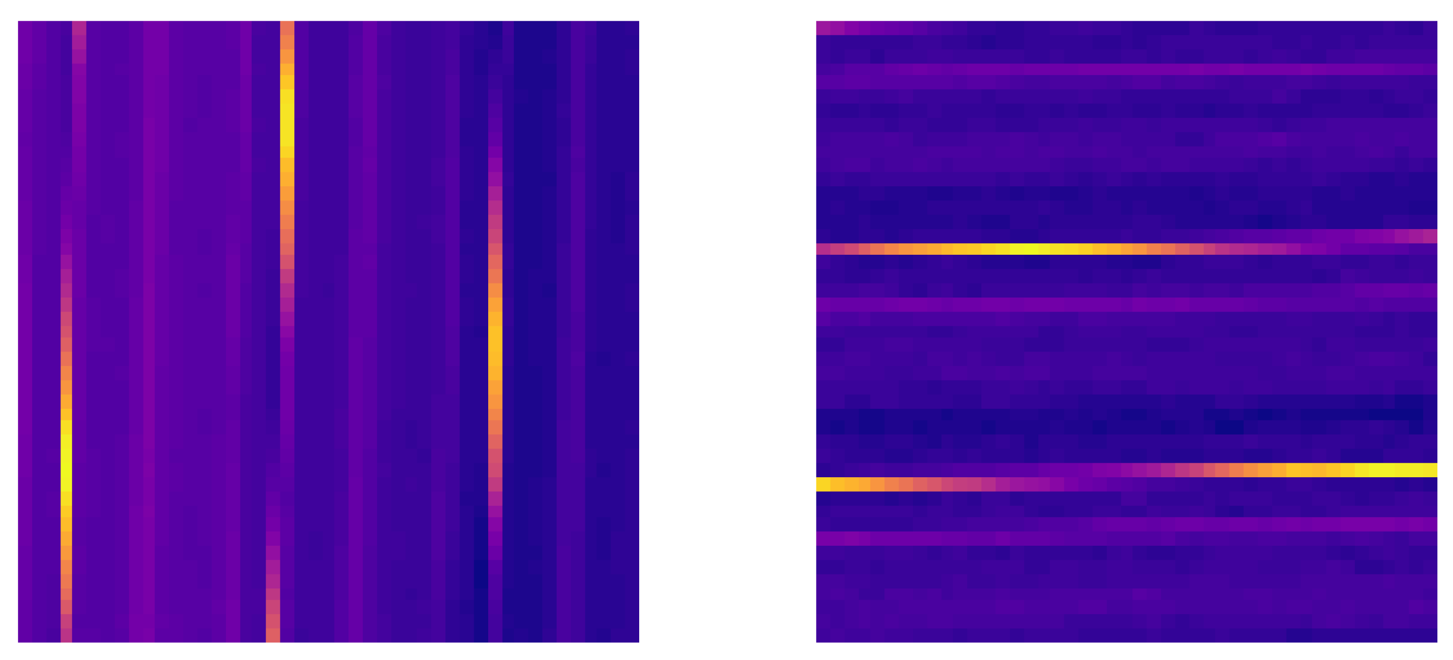
The objective of this short study is to check whether the arrangement of the elements of the time series can affect the performance of the GAN. Two configurations are tested for the arrangement derived from the original one: for the transposed configuration data will follow a movement from up to down, then left to right. For the reversed layout, data will be arranged following a reversed “Z” movement starting from the bottom right pixel. Both configurations can be seen in Figure 10.
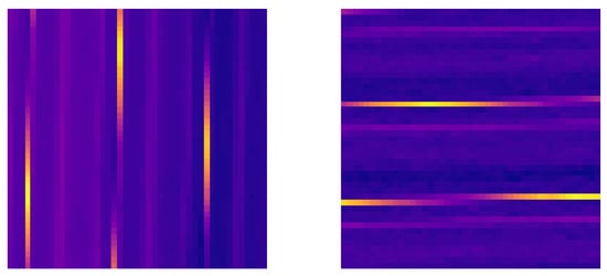
Figure 10.
(Left) A ground truth example for the transposed model. (Right) A ground truth example for the reversed model.
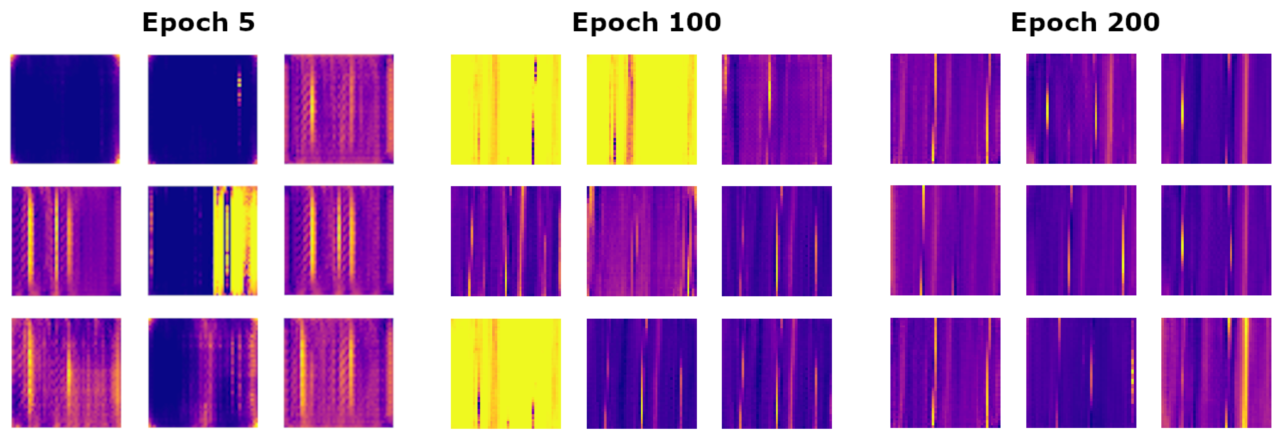
For both configurations the obtained results are very similar to the original ones in [10]. Figure 11 shows the evolution of the outputs along the training epochs for the transposed arrangement. As in the original model, in epoch 100 some samples already have a pattern similar to real samples but there are still some of them that have a different scale, like the yellow ones. Finally, in epoch 200, all images have the same pattern than the original one.

Figure 11.
Generated Cardiogram images samples in transposed arrangement through 200 epoch training with a CNN model.
Regarding the shape of the generated electrocardiogram samples (see Figure 12 (left)), there are slight differences with those generated by the original “Z” model: in two samples (top right and middle left) the generated time series is more noisy than the original ones and the peaks generated seem to be more irregular. For the reversed configuration, the results are very similar to both, the transposed one and the original one, with a similar evolution of the outputs along the epochs. The generated electrocardiograms shown in Figure 12 (right) are more similar to the original ones than those from the transposed arrangement. There are equidistant pulses in almost all images, there are two or three peaks in all images (but still with different heights) and the slope is constant during the sample. In conclusion, there are no significant differences between the generated samples of the original model and the two new models.
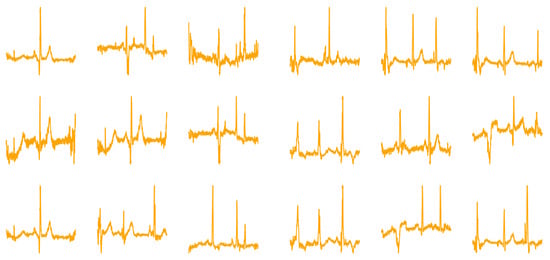
Figure 12.
(Left) Generated samples for the transposed model. (Right) Generated samples for the reversed model.
Finally, let us note that the objective of kernels in CNNs is to extract the dominant features from the images, for example the peaks. New results could be obtained whether some parts of the signal with similar shapes are put together in the data arrangement. This could be performed, for instance, in the frequency domain.
4.3. RGB Data Arrangement
Until now, information has been arranged in only one channel (one image) by aggregating features for the static data (thyroid database) or considering only one-dimensional time series for the dynamic case (cardiogram database). In case that more signals should be arranged, they can be aggregated or concatenated in one channel. However, a mainstream when considering CNN is to work with tensors, that is several channels convoluting information into the original image. A different solution will be provided in this study by inserting images to the GAN on three channels. Until now, even though all the displayed images are coloured, like purple, blue and yellow, GAN architecture was not working with coloured images. Indeed, all images are being processed in grayscale.
To introduce colour into the model, RGB images will be feed to it. RGB is an abbreviation of the terms “Red”, “Green” and “Blue” and is a chromatic model through which all colours can be represented with a combination of those three. RGB images are composed of overlapping three layers, each of them with a colour associated. These colours go from a value 0 to a value 255 in decimal notation.
Besides the signal ‘i’ that has been used until now, two more of signals from Figure 5 (left) will be included, signal ‘ii’ and signal ‘iii’, which correspond to the second and third signal of a conventional electrocardiogram, respectively. It is important to mention that even though signals are recorded with different sensors, all of them are related because they are recorded at the same time and capture different features of the same heartbeat. Consequently, some relationship appears with the different samples, for example, when in the signal ‘i’ appears a peak, in signal ‘ii’, appears as well. Signal ‘i’ will be stored in the red channel, signal ‘ii’ in the green channel and signal ‘iii’ in the blue channel. Every channel has the same shape and structure than the original model: a shape of and the arrangement of the pixels is the one following a “Z” movement from left to right, then up to down. It is shown in Figure 13 the combination of the three individual channels or signals which together create an RGB image.

Figure 13.
A ground truth RGB image as a combination of three channels, each of them with an electrocardiogram signal.
The configuration of the layers is similar to the original model. Both discriminator and generator are endowed with four layers. Now, however, the discriminator in the first layer is not considering only one channel or dimension () as the input, but three channels (). Similarly for the generator, its output is composed of three channels instead of having just one. The configuration of the hidden convolution layers does not change.
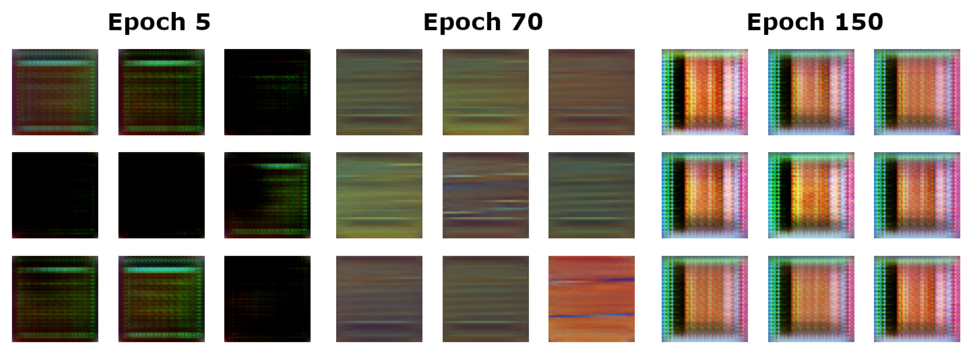
Starting with a set-up for the GAN architecture training similar to the one for the one-channel solution, a stable GAN was unable to be obtained. At a certain point in the learning procedure, the mode collapse problem appeared. That is, the generator learns to produce only a limited range of outputs, sometimes with unrealistic results. Hence, the discriminator gets stuck in a local minimum and the generator over-optimizes for this particular discriminator. As a result, the generators rotate through a small set of output types.
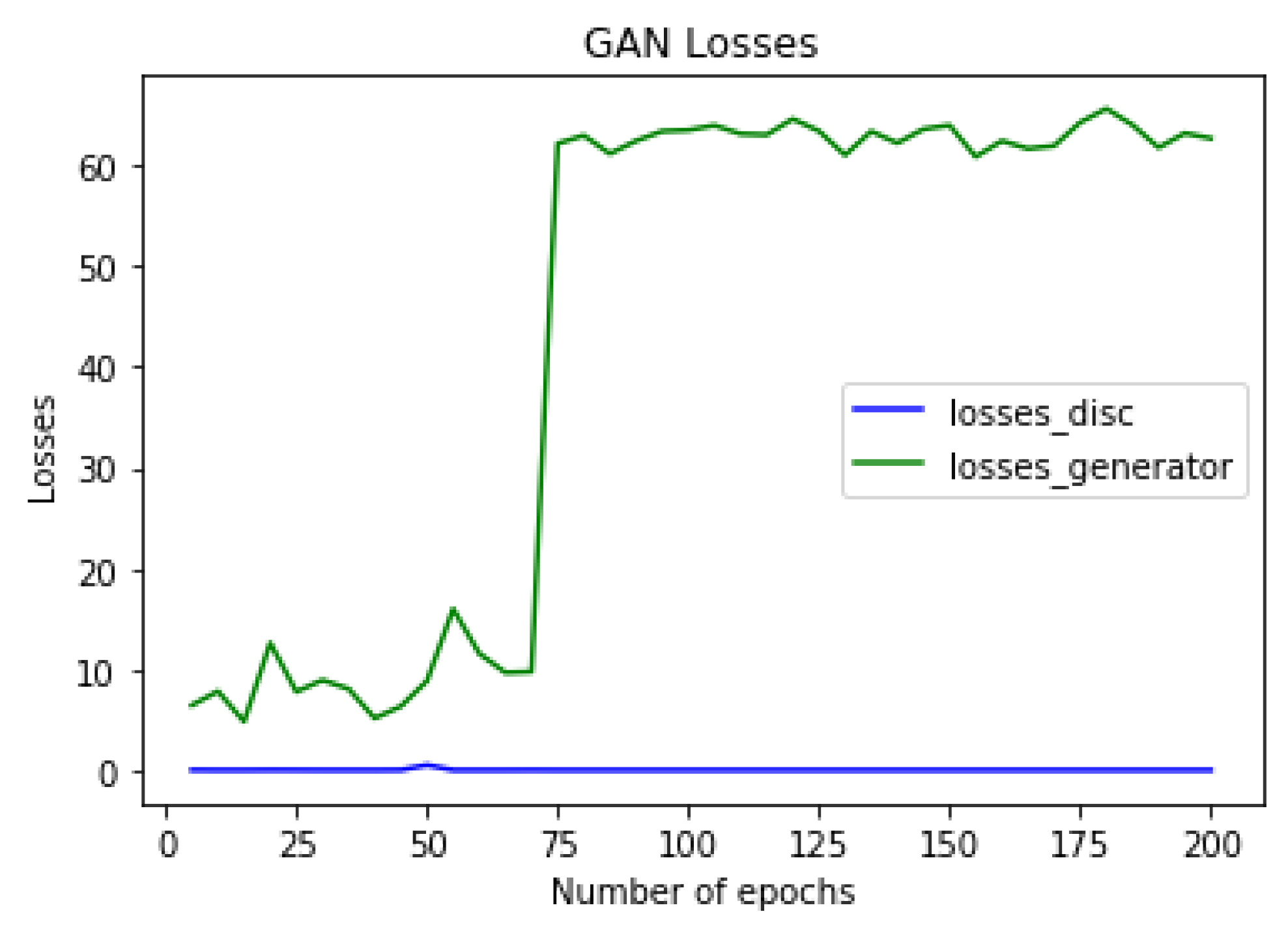
As it can be observed in Figure 14, from epoch 75 until epoch 150 the generated images follow always the same pattern: a random image with a lot of noise. The losses record for the model in Figure 15 shows the GAN architecture working correctly until it gets to epoch number 75, where it starts with mode collapse and all the losses of the generator oscillate around a constant number.
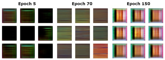
Figure 14.
Evolution of the samples created using the RGB arrangement for three signals.
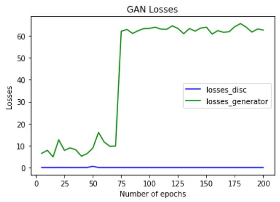
Figure 15.
Losses record for the RGB arrangement. Mode collapse can be observed after epoch 75.
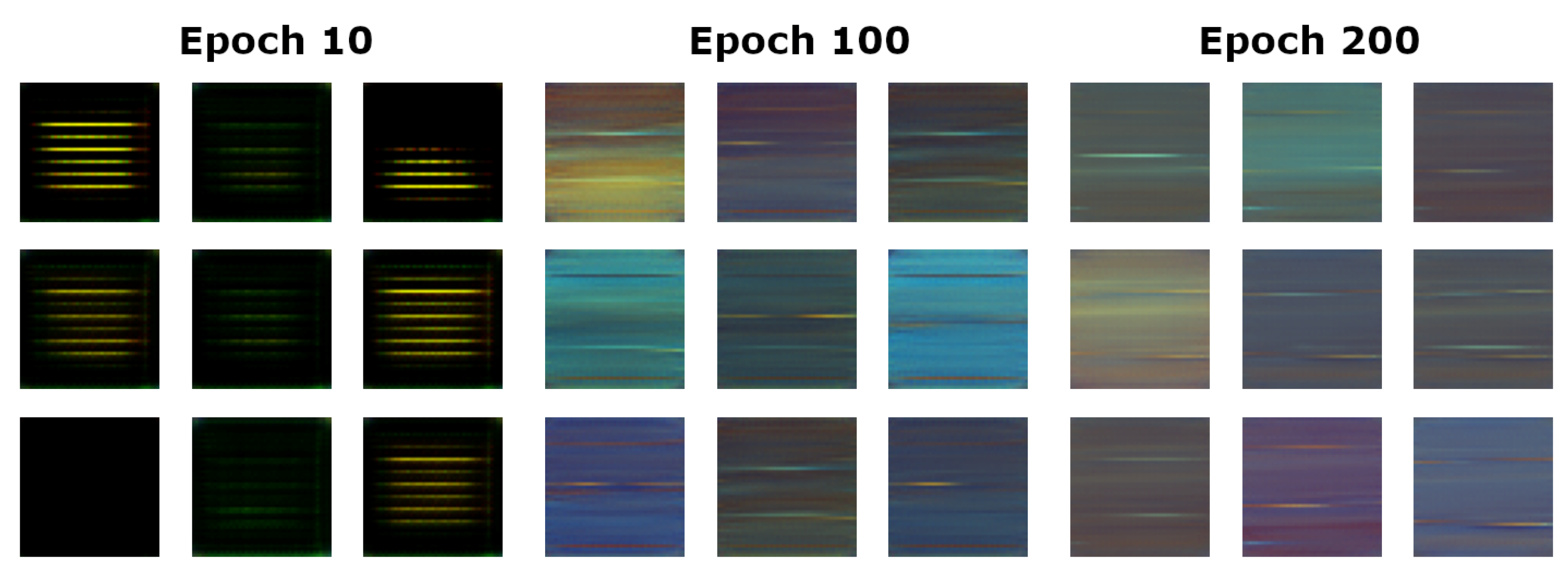
Some authors [13] suggest that a larger batch size drives to a degradation in the quality of the model, but reduces the probability to get mode collapse. For this reason, batch size is changed from 30 images to 60 images per batch. Then, GAN avoids mode collapse and generates results. Figure 16 shows the images created in epochs 10, 100 and 200. These images built on three layers, one channel per layer. As in the one-channel case, in epoch 10 generated images are very similar and a lot of noise appears. Images created in epoch 100 are already consistent and similar to the ones generated in epoch 200.
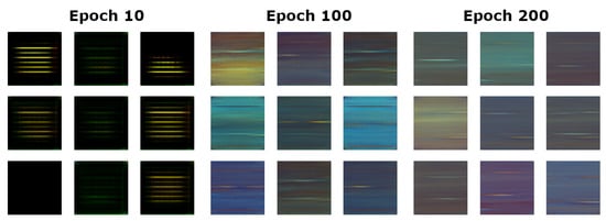
Figure 16.
Evolution of the samples created in the final RGB model.
When these images are transformed into a time series again, as shown in Figure 17, they get the shape of a possible electrocardiogram (three first signals), but more noisy than in the original samples. Two random real samples (in blue) are shown along with some synthetic (in orange) generated samples of electrocardiogram data. By comparing, it can be observed that the relationship between the three channels is hold in the synthetic samples, keeping the same pattern for the three samples. Hence, the peak appears at the same time at the three signals in the first sample. However, in that sample there only appears one peak, when usually there are two or even three. In the second sample some noise appears in the first signal, but the shape of a normal electrocardiogram can be seen. Additionally, in signal ‘ii’ and signal ‘iii’ the slope is constant and the same in the two signals. Finally, the third one has a first part where signals have a normal shape, doing the down peak in the third signal, but then the second part does not present a realistic shape. In conclusion, there has been a successful implementation in the form of RGB images, introducing three channels instead of one in the input of the discriminator and the output of the generator. The images generated are consistent, but the quality of the signals could be much better: shapes have sometimes strange patterns and there is more noise than in the previous models.

Figure 17.
(Left) Three generated electrocardiograms after 200 epoch using the RGB data arrangement for three channles. (Right) Two original samples from the Cardiogram database.
4.4. Concatenated RGB Data Arrangement: Six Channels
As mentioned previously, the original one-channel image arrangement can be extended to three channels using the proposed RGB approach. Moreover, multi-channel arrangement can be obtained by simply concatenating signals.
Despite having a regular losses record with the same shape as previous models, the generated electrocardiograms are not good enough. As it can be seen in Figure 18, the generated samples are still too noisy waves, and resemblance with electrocardiograms is still far. In conclusion, GANs are good tools for processing and generating new images, generally using images in RGB mode (three channels). When introducing six channels at the same time, the GAn architecture accepts signals concatenation without problems, but then results are not as good as expected. It could be that the architecture used with three channels applied to six channels may not be the most suitable, and a new one should be used by making appropriate changes. Either, it is only a matter to increase the number of epochs.
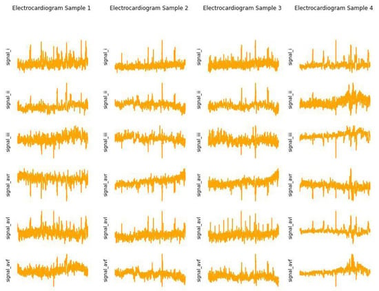
Figure 18.
Generated electrocardiograms for the model.
4.5. Training Concerns: Label Smoothing
In most of the previous analyzed experimental GAN architectures the discriminator is behaving overconfident, only relying on a very limited set of features to determine its output. This is usually the case with hard targets: the model should produce large logit value for the correct label, decreasing its ability to adapt, in turn, leading to overfitting.
It is suggested in [14] to use label smoothing as a solution, that minimizes cross-entropy using soft targets by relaxing the confidence on the labels lowering the loss target values. In fact, it is recommended using one-sided smooth labelling, which means only smooth discriminator values and also smooth only real samples, by lowering loss targets values from 1 to 0.9. It is empirically shown in [15] that label smoothing improves model calibration and robustness.
The data arrangement method employed to test label smoothing is the three-channels RGB model with real samples of the discriminator reducing the label to 0.9. The variety of samples generated along a 200 epochs training is wide bigger than the one from the original RGB model, where most of the images generated have similar shapes, colours and patterns. Furthermore, the quality of electrocardiograms, as it can be seen in Figure 19, improves that in Figure 17: samples have less noise and signals have shapes more identifiable as the typical ones of electrocardiograms. These differences, however, are qualitative and cannot be quantified with the losses record. Additionally, the relationship between the three signals in all samples is more evident: when there are peaks up in the signals ‘i’ and ‘ii’, signal ‘iii’ produces a peak down, as happens in general in the ground truth samples.

Figure 19.
Generated electrocardiograms after 200 epoch training using the RGB data arrangement with label smoothing.
4.6. A Classifier GAN as an Indirect Performance Measure
In personalised health, GAN-based models are built to characterize user’s illness/healthy behaviours, that is classification issues. In this study, a classifier GAN model will be tested, hence merging synthetic data generation and classification. The objective for the architecture is, primarily, to differentiate electrocardiograms depending on which kind of disease the patient suffers. Moreover, we will check that popular measures in classification such as Accuracy provide an excellent, but not perfect, indirect performance measure for the quality of the generated images, beyond the current qualitative visual inspection.
The ACGAN or Auxiliary Classifier Generative Adversarial Network [16] is selected for this study because its simplicity, but many other similar architectures could be employed. It consists of a standard GAN system, then a classifier is added so the GAN-based architecture accomplishes two tasks: the main task is to generate synthetic images, then a second task is to classify them in classes. Hence, in ACGAN each sample contains also the class label, which should be also generated along the images. On the one hand, the generator is fed with both the class and the seed vector and generates synthetic samples images. On the other hand, the discriminator is endowed with two parallel final layers, a linear layer with sigmoid activation to differentiate between real or synthetic, and a linear layer with a softmax activation, to differentiate between classes.
Since two outputs are now under consideration (image source and class), the losses are modified in two parts, the log-likelihood for the source , and the log-likelihood for the class ,
where generated images are represented as , real images are , S stands for source (image in our case) and C stands for class. The discriminator is trained to maximize , the class loss and the source loss, and the generator is trained to maximize , which means that tries to maximize the class loss and also minimize the source loss.
Information about classes is also contained in the Physionet database as summarized in Table 1. There can be seen that 8 different diagnostics are possible, along with some miscellaneous diagnostics. The column ‘Samples’ shows how many full electrocardiograms are in the database for each class. As it takes a lot of images (thousands) to train the model and most of the classes have just a few number of samples, the number of classes is reduced to just three: ‘Myocardial infarction’, ‘Healthy control’, and ‘Miscellaneous’ by grouping all the other classes not included in this classification. In Table 2 is presented a summary of the three classes remaining, with the number of full electrocardiograms. The column ‘Sliced samples’ shows how many samples are to train the model. Each sample is a slice of the full electrocardiogram of size 2025, which corresponds to an image of pixels.

Table 1.
Number of electrocardiograms samples by diagnostic class in Physionet.

Table 2.
Number of electrocardiograms samples, number of sliced electrocardiograms and class number for the three diagnostics.
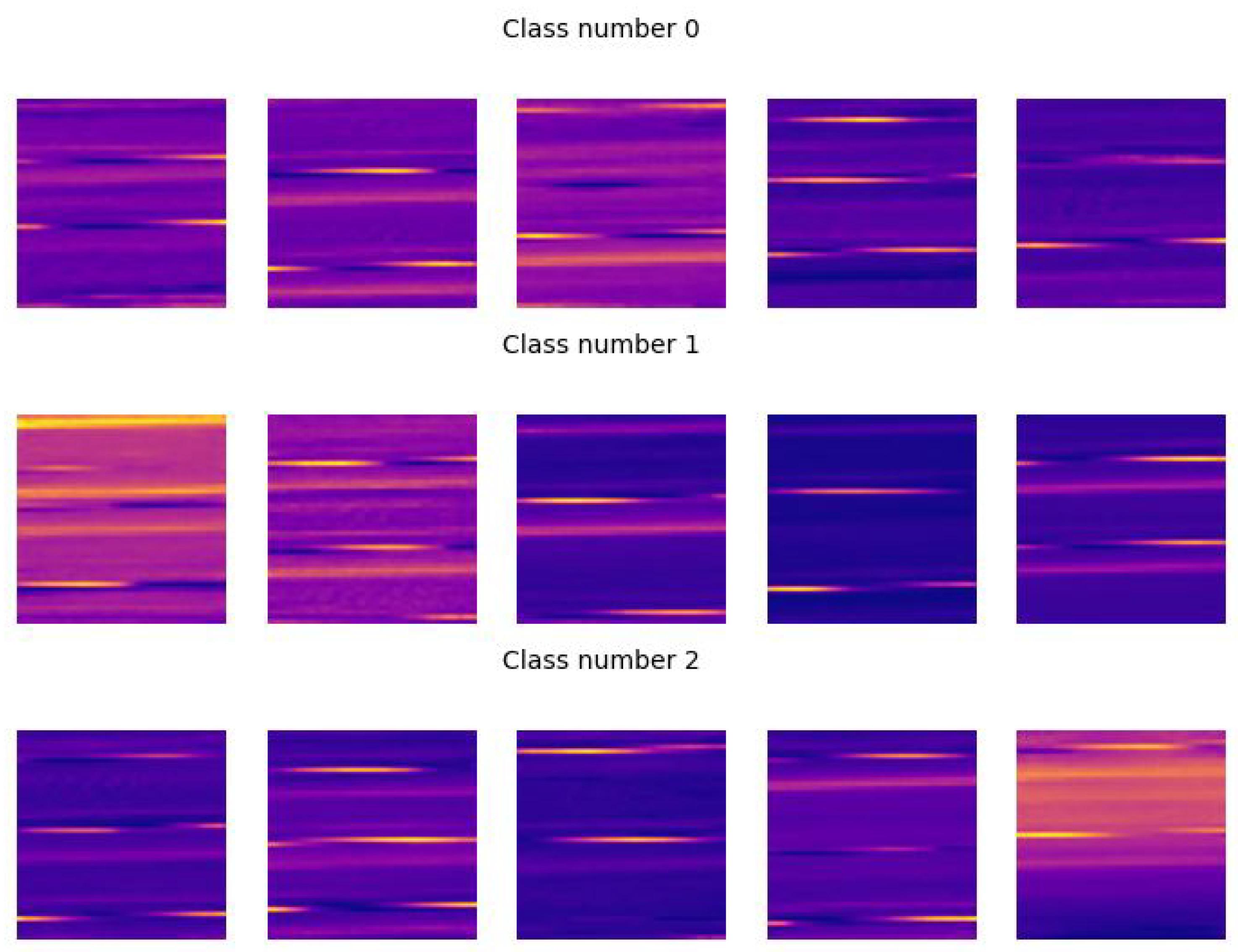
The iteration process to train the model is the same as the precedent ones. The model is trained with only one channel (signal ‘i’) and images sized . The batch size is set to 30. Again, as usual, initial attempts to train the model are not successful ending up in mode collapse, between epochs 70 and 100. Some changes are considered: the batch size is augmented to 64 and smooth labelling is included, applied to the discriminator only when is evaluating the real samples. Finally, as the model was lighter and quicker than RGB models, it was trained through 400 epochs. Next, the new model is trained and a new problem appears: correct shapes are produced only for the class 0 (‘Myocardial Infarction’). This problem is due to the imbalance between the three classes. The class 0 has significantly more samples, five times, in the training set than other classes, hence the learning algorithm biases towards the majority class. To solve this problem, an under-sampling strategy is followed: the two classes having more samples are reduced to the size of the one which has less, ‘Healthy control’ class, with 4390 samples. The samples chosen to be extracted have been picked up randomly. Finally, after all these changes, the same model leads to satisfactory results. Figure 20 shows the time series of the three classes as generated images.
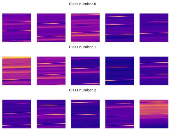
Figure 20.
Generated images for the ACGAN model after 400 epochs training.
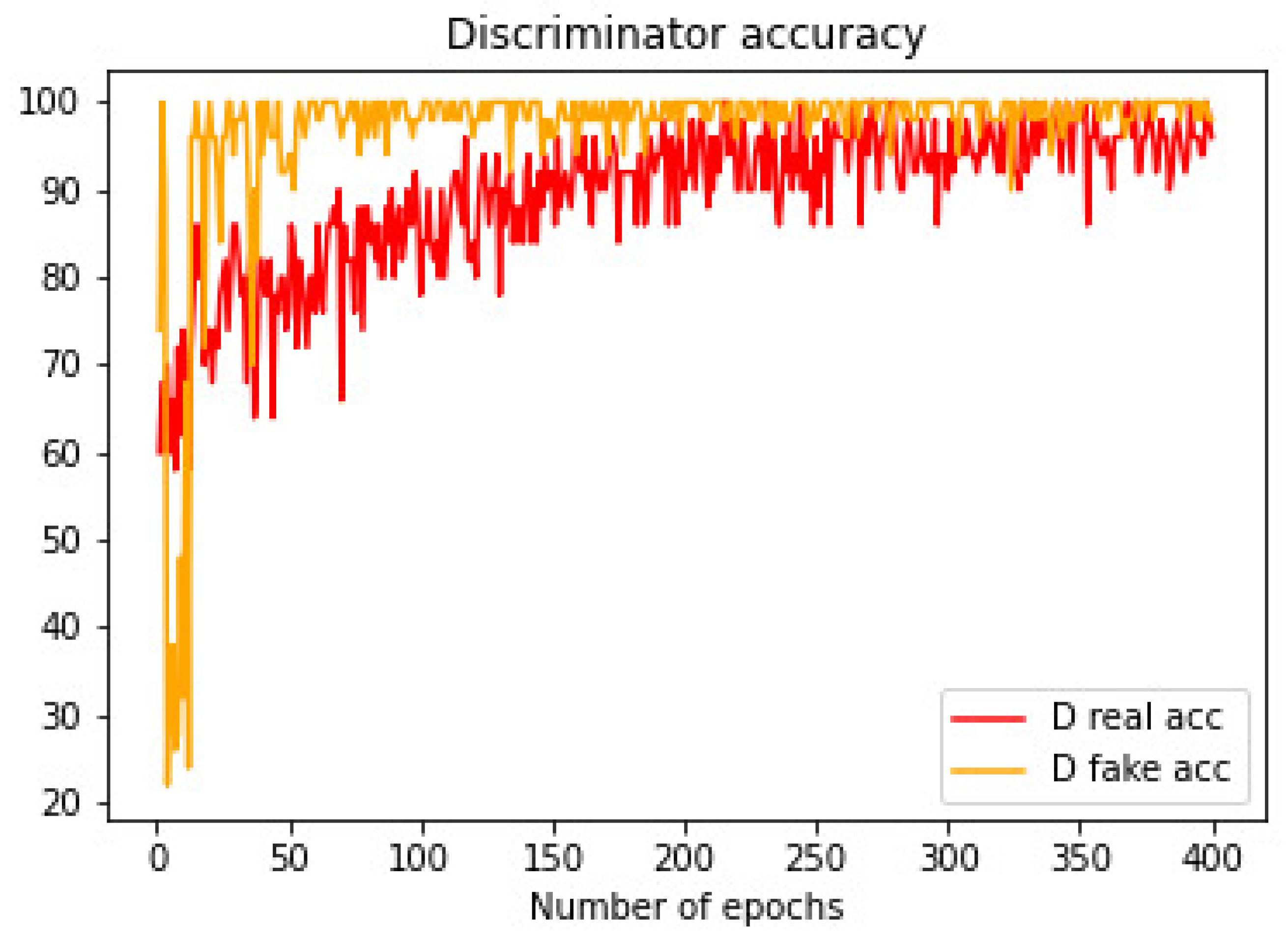
The use of the ACGAN architecture allows to check our GAN-based anonymized system under a posterior task, a classification. Now, we can go beyond visual checking of synthetic ECGs and get an indirect proof for the good performance of the proposed architecture using the Accuracy measure for the discriminator in the classification task. In Figure 21 it is shown the accuracy of the discriminator along 400 epochs, for both, real (red) and synthetic (yellow) samples. The discriminator starts with low accuracy for the synthetic samples, around 30–40%, which is the same as if it was randomly performed. However, before epoch 50 it succeeds to get a very high accuracy. For the real samples, accuracy starts with a better percentage. Eventhough the increase rate is lower, a high accuracy is also obtained, reaching the highest values near epoch 300.

Figure 21.
Accuracy of the discriminator for real and synthetic samples.
4.7. On Evaluation Measures and Training Stopping Criteria
In the previous study we are able to indirectly measure the performance of our GAN-based anonymization system by checking the Accuracy measure in the discriminator in a parallel classification task on the real and synthetic images. However, the fact that the discriminator can successfully classify synthetic samples does not mean that the quality of the samples is good enough ‘per se’, but that they are different enough from each other for it to be able to classify them. In this short theoretical study we will elaborate on current measures checking the performance of GANs and we will show that our indirect Accuracy measure on a parallel classification task is the current state-of-the-art in GAN performance’s measures. Moreover, it is also an excellent training stopping criterion, beyond the current visual inspection.
One of the most common troubles that GAN developers face is when to stop model training. Theoretically, the stop criteria should be the moment that the model reaches Nash equilibrium. At that moment, the discriminator, and the generator, gets an accuracy of 50%, because the quality of the synthetic images is so good that the generator fools the discriminator. However, most of the times this situation can not be observed in the losses of both networks. In Reference [17], it is claimed that GANs may, and usually, never arrive at this point, but in simpler cases. This is the situation we face in our GAN structure.
As a second possibility, you should at least to ensure convergence, that is the discriminator and the generator reach a certain equilibrium, but not the Nash one. This situation happens when one network (discriminator or generator) will not change its action regardless of what the opponent may do. However, in this case, the equilibrium means that the discriminator overtakes the generator, or reversely. In both situations, you can not ensure convergence but not a good quality for the generated images. Sometimes the equilibrium (convergence) is reached and the produced images are visually correct, sometimes are not. Hence, the only way to stop the GAN training is by visually inspecting the generated images and stop if there is no visually perceived improvement in them.
The quality of the images generated is a qualitative measure, depending on every person that analyses the images, so it is difficult to determine when the generator should stop while generating good enough images. Furthermore, most of the times the quality is not related to the loss functions, because a huge improvement in the quality may not be reflected in a reduction of the loss. It can also happen that the generator cost increases and the image quality improves. Hence, the objective function or losses of the GAN determines the good behaviour of the generator or discriminator concerning its opponent, but it does not represent the quality or diversity of the result. Consequently, metrics are needed that can measure these characteristics.
In Reference [18], twenty-four quantitative techniques for evaluating GAN generator models are gathered, among which the most used are the Inception Score (IS) [14] and the Frechet Inception Distance (FID) [19]. The Kernel Inception Distance (KID) was latter introduced in [20]. In all the cases, these measures are defined only when using the pre-trained deep learning neural network model Inception for image classification, which is not our case, neither for most of GAN-based structures. In conclusion, these direct measures can help to decide when to stop training a GAN, but one can not make this decision just looking at one of these measures, as image quality is not directly related, similarly to our indirect Accuracy measure on a parallel classification task. Consequently, the stop criteria is still a combination of several factors: visually inspecting the quality of the images generated, looking at the losses record to detect failures like mode collapse, and using measures to compare mathematically the difference between the real and the synthetic samples.
5. Discussion
This paper elaborates on a first approach about using Generative Adversarial Networks (GANs) for the generation of synthetic data, with the objective of anonymizing users information in the health sector, especially in the case of ECGs, a multi-dimensional dynamical system with a raw/image data dual definition. As a first result, a general procedure is provided to convert original usual raw data into images, which are more fitted to work with GANs. Next, a GAN structure is determined, trained and evaluated. Hence, a five-steps procedure is proposed: (i) data standardization, (ii) data arrangement into an image, (iii) GAN-based architecture selection, (iv) training concerns, and (v) results evaluation.
Firstly, from very recent precedent work it is demonstrated that our proposed GAN system, using standard GAN architectures, is able to get good results on anonymization for personal data on general health data. Next, several studies are proposed along the five-steps procedure exploring the GAN-based anonymization original solution.
5.1. Data Standardization
In this case, usual exploratory data analysis concerns are under consideration in our study: outliers detection using quantiles, data normalization in the range , rigid vs. mobile normalization for the different dimensions in the multidimensional time series. More complicated computer vision techniques as histogram equalization for image contrast enhacement, among others, are left as future research in the computer vision domain because they are far of our current study.
5.2. Data Arrangement into an Image
Firstly, simple data arrangements of uni-dimensional time series are considered in the form of a “Z” shape, its transposed and its reversed configurations. Similarly, many different simple arrangements are possible, including randomized ones. For the three simple data arrangements under study, no significant differences were found when generating synthetic samples under similar training regimes.
It could be argued that there already exist solutions that can be used to generate these kind of signals working on 1D ECG signals, hence avoiding the use of images. However, there are many reasons to employ our image-based approach. Firstly, we are not introducing almost computational cost, since the image conversion is straightforward. Moreover, we are gaining all the power and previous experience on GANs working on images. In particular, the proposed arrangements could take into consideration the special nature of the time series under consideration, for instance periodicity, special frequencies, working zones, and so on. Finally, ECGs are multi-dimensional systems, hence working separately 1D ECG signals will prevent to capture the multi-dimensional nature of the system.
Next, a tricky three-dimensional RGB-based data arrangement into an image was introduced. This arrangement allows to convert time relationships between time series into color relationships. For the ECGs, displacement in the peaks for the three signals under consideration are converted into different color codification, hence it is visually more obvious to check this feature. Again, “Z” shape and easy derivations of this configuration can be considered at start, then moving to more complicated ones. Moreover, the RGB codification is not the only one to be considered. Other color spaces as HSV/HSB, CMYK, CIE-LAB, among others, can be studied and the obtained results be analyzed.
Finally, dimensions in the time series were also concatenated to build a six channels image. Concatenation is again an easy arrangement to joint several dimensions in a time series or several features in a database. However, this is not the only one mixing arrangement that can be considered. Stripes, squares, and randomized shapes can be also under consideration, especially whether special relationships between channels want to be highlighted.
5.3. GAN-Based Architecture Selection
In our study, only standard fully connected networks and convolutional neural networks under similar training regimes were under consideration. This straightforward selection for the GAN architecture was done on purpose, to maintain the main focus of our research on the synthetic generated samples. Architecture selection is a key step in the defined five phases procedure to obtain valid synthetic ECGs. A lot of improvements and extensive studies can be performed in this direction in the near future.
5.4. Training Concerns
Usual training concerns appear in our experimental work when training standard GAN architectures for the arranged images. Mode collapse and vanishing gradients being the most popular ones. Batch size increase and label smoothing were appropriate solutions in this case to manage these training problems. Again, depending on the chosen GAN architecture and the training hyper parameters selection, many modifications and techniques can be took into consideration in further research.
5.5. Results Evaluation
When working with GAN architectures, the evaluation of results and the training stopping criterion are very dependent on visual inspection techniques, most of them imported from the computer vision research area. In the case of using Inception as pre-trained model, then several indirect measures (scores and distances) have been defined on the convolutional layers, but this is not the general case, neither our experimentation setup.
In this article a new indirect performance measure have been defined that does not depends on visual inspection. Based on checking the accuracy for a parallel classification task, it allows to indirectly check the performance of the GAN system when generating synthetic ECGs as well as determine a stopping criterion. It can be applied only for the case that data is labelled and suffers of similar problems to the other indirect performance measures defined for the use of the pre-trained Inception layer: it ensures convergence of the GAN architecture, but it does not means that generated images are good enough from a visual inspection approach. More work should be still developed for measuring GAN performance when generating new images. However, we are providing in this work a new technique that is valid for many cases, especially supervised classification.
5.6. Applications and Ethics Concerns
The introduced architecture for generating ECGs images is a very useful tool as it is enabling unlimited similar-to-the-original data without compromising the privacy of the original elements. The applications of this tool range from educational purposes with young health professionals [21] to scientific simulations and investigations using synthetic signals for the training of automatic systems for the detection of heart disease [22].
Employing results from a GAN designed for synthetic data generation without proper expert evaluation and approval is unethical. The generated images can be employed for data augmentation or any other health-related application only in the case that some expert is authorising they are representative enough from the perspective of physical/physiological features. It is not enough that they are following the original data distribution. For this reason, it is not declared that we are imitating or learning ECGs, but generating synthetic/fake ECGs. It should be clearly indicated that generated synthetic data will be employed only after expert evaluation and approval.
Author Contributions
Conceptualization, C.A.; methodology, C.A., E.P. and A.G.; software, E.P. and A.G.; validation, C.A., E.P. and A.G.; formal analysis, C.A.; investigation, E.P. and A.G.; resources, E.P. and A.G.; data curation, E.P. and A.G.; rriting—original draft preparation, C.A.; visualization, E.P. and A.G.; project administration, C.A.; funding acquisition, C.A. writing—review and editing, C.A. All authors have read and agreed to the published version of the manuscript.
Funding
This research was partly funded by the Spanish Ministry of Science, Innovation and Universities (AEI/FEDER, UE) grant number PGC2018-102145-B-C22 (research project EDITH) and co-financed by the European Regional Development Fund of the European Union in the framework of the ERDF Operational Program of Catalonia 2014–2020 with a grant of €1,331,903.77, grant number 001-P-001643. Prof. Cecilio Angulo has been partly supported by the European Union’s Horizon 2020 research and innovation programme under grant agreement No. 825619 (AI4EU).
Data Availability Statement
Data supporting reported results can be found in links provided along the article.
Conflicts of Interest
The authors declare no conflict of interest.
References
- Morillo, L.M.S.; Gonzalez-Abril, L.; Ramirez, J.A.O.; De la Concepcion, M.A.A. Low Energy Physical Activity Recognition System on Smartphones. Sensors 2015, 15, 5163–5196. [Google Scholar] [CrossRef] [PubMed]
- Angulo, C.; Ortega, J.A.; Gonzalez-Abril, L. Towards a Healthcare Digital Twin. In Frontiers in Artificial Intelligence and Applications; Sabater-Mir, J., Torra, V., Aguiló, I., González-Hidalgo, M., Eds.; IOS Press: Oxford, UK, 2019; Chapter Volume 319, pp. 312–315. [Google Scholar]
- Bruynseels, K.; Santoni de Sio, F.; van den Hoven, J. Digital Twins in Health Care: Ethical Implications of an Emerging Engineering Paradigm. Front. Genet. 2018, 9, 31. [Google Scholar] [CrossRef] [PubMed]
- El Emam, K.; Arbuckle, L. Anonymizing Health Data: Case Studies and Methods to Get You Started, 1st ed.; O’Reilly Media, Inc.: Newton, MA, USA, 2013. [Google Scholar]
- Feutry, C.; Pablo Piantanida, Y.B.; Duhamel, P. Learning Anonymized Representations with Adversarial Neural Networks. arXiv 2018, arXiv:1802.09386. [Google Scholar]
- Goodfellow, I.; Pouget-Abadie, J.; Mirza, M.; Xu, B.; Warde-Farley, D.; Ozair, S.; Courville, A.; Bengio, Y. Generative Adversarial Nets. In Advances in Neural Information Processing Systems 27; Ghahramani, Z., Welling, M., Cortes, C., Lawrence, N.D., Weinberger, K.Q., Eds.; Curran Associates, Inc.: New York, NY, USA, 2014; pp. 2672–2680. [Google Scholar]
- Shao, S.; Wang, P.; Yan, R. Generative adversarial networks for data augmentation in machine fault diagnosis. Comput. Ind. 2019, 106, 85–93. [Google Scholar] [CrossRef]
- Li, S.C.X.; Jiang, B.; Marlin, B. MisGAN: Learning from Incomplete Data with Generative Adversarial Networks. arXiv 2019, arXiv:1902.09599. [Google Scholar]
- Piacentino, E.; Angulo, C. Anonymizing Personal Images Using Generative Adversarial Networks. In Bioinformatics and Biomedical Engineering; Rojas, I., Valenzuela, O., Rojas, F., Herrera, L.J., Ortuño, F., Eds.; Springer International Publishing: Cham, Switzerland, 2020; pp. 395–405. [Google Scholar]
- Piacentino, E.; Angulo, C. Generating Fake Data Using GANs for Anonymizing Healthcare Data. In Bioinformatics and Biomedical Engineering; Rojas, I., Valenzuela, O., Rojas, F., Herrera, L.J., Ortuño, F., Eds.; Springer International Publishing: Cham, Switzerland, 2020; pp. 406–417. [Google Scholar]
- Kumar, A.; Passi, A. Comparison and combination of iris matchers for reliable personal authentication. Pattern Recognit. 2010, 43, 1016–1026. [Google Scholar] [CrossRef]
- Barnett, S.A. Convergence Problems with Generative Adversarial Networks (GANs). arXiv 2018, arXiv:1806.11382. [Google Scholar]
- Keskar, N.S.; Mudigere, D.; Nocedal, J.; Smelyanskiy, M.; Tang, P.T.P. On Large-Batch Training for Deep Learning: Generalization Gap and Sharp Minima. arXiv 2016, arXiv:1609.04836. [Google Scholar]
- Salimans, T.; Goodfellow, I.; Zaremba, W.; Cheung, V.; Radford, A.; Chen, X. Improved Techniques for Training GANs. arXiv 2016, arXiv:1606.03498. [Google Scholar]
- Müller, R.; Kornblith, S.; Hinton, G. When Does Label Smoothing Help? arXiv 2019, arXiv:1906.02629. [Google Scholar]
- Odena, A.; Olah, C.; Shlens, J. Conditional Image Synthesis With Auxiliary Classifier GANs. arXiv 2016, arXiv:1610.09585. [Google Scholar]
- Farnia, F.; Ozdaglar, A. GANs May Have No Nash Equilibria. arXiv 2020, arXiv:2002.09124. [Google Scholar]
- Borji, A. Pros and Cons of GAN Evaluation Measures. arXiv 2018, arXiv:1802.03446. [Google Scholar] [CrossRef]
- Heusel, M.; Ramsauer, H.; Unterthiner, T.; Nessler, B.; Hochreiter, S. GANs Trained by a Two Time-Scale Update Rule Converge to a Local Nash Equilibrium. arXiv 2017, arXiv:1706.08500. [Google Scholar]
- Lakhey, M. Generative Adversarial Networks Demystified. Medium Data Driven Investor 2019. Available online: https://medium.com/datadriveninvestor/gans-demystified-f057f5e32fc9 (accessed on 10 November 2020).
- Goncalves, A.; Ray, P.; Soper, B.; Stevens, J.; Coyle, L.; Sales, A.P. Generation and evaluation of synthetic patient data. BMC Med. Res. Methodol. 2020, 20, 108. [Google Scholar] [CrossRef] [PubMed]
- Dutta, A.; Batabyal, T.; Basu, M.; Acton, S.T. An efficient convolutional neural network for coronary heart disease prediction. Expert Syst. Appl. 2020, 159, 113408. [Google Scholar] [CrossRef]
Publisher’s Note: MDPI stays neutral with regard to jurisdictional claims in published maps and institutional affiliations. |
© 2021 by the authors. Licensee MDPI, Basel, Switzerland. This article is an open access article distributed under the terms and conditions of the Creative Commons Attribution (CC BY) license (http://creativecommons.org/licenses/by/4.0/).

