Abstract
Recently, the demand for monitoring a certain object covering large and dynamic scopes such as wildfires, glaciers, and radioactive contaminations, called large-scale fluid objects (LFOs), is coming to the fore due to disasters and catastrophes that lately happened. This article provides an analytic comparison of such LFOs and typical individual mobile objects (IMOs), namely animals, humans, vehicles, etc., to figure out inherent characteristics of LFOs. Since energy-efficient monitoring of IMOs has been intensively researched so far, but such inherent properties of LFOs hinder the direct adaptation of legacy technologies for IMOs, this article surveys technological evolution and advances of LFOs along with ones of IMOs. Based on the communication cost perspective correlated to energy efficiency, three technological phases, namely concentration, integration, and abbreviation, are defined in this article. By reviewing various methods and strategies employed by existing works with the three phases, this article concludes that LFO monitoring should achieve not only decoupling from node density and network structure but also trading off quantitative reduction against qualitative loss as architectural principles of energy-efficient communication to break through inherent properties of LFOs. Future research challenges related to this topic are also discussed.
1. Introduction
With an increasing number of various (wireless) sensor devices connected to the Internet, it is possible to obtain the infrastructural and environmental data that would enable efficient approaches to perceive and manage urban facilities [1]. Such a new paradigm paving the way to realize urban sensing is called Internet of Things (IoT) and many cities have deployed sensor platforms to support urban sensing. IoT infrastructure could facilitate a wide variety of applications in urban environments such as commercial asset tracking, disaster emergency response, urban internet, intruder detection [2]. In other words, sets of sensor devices would be connected for monitoring power plants for smart grid, mountains in cities, transportation systems, smart homes, and so on.
Wireless sensor devices are deployed on a targeted field where target objects exist and remotely monitor events or phenomena the objects trigger [3,4]. For instance, a number of sensor nodes could be set up over a target region for intruder detection [2]. Then, when the sensor nodes detect the intrusion event, they report sensing data to a base station, commonly called a sink. For such monitoring applications, previous studies [4,5] typically assume that events or phenomena are generated by individual mobile objects (IMOs) such as vehicles, people, and animals. The previous studies mainly make an effort to disseminate sensory data into a sink in energy-efficient means since energy efficiency is the core design principle of systems based on low-cost energy-constrained sensor nodes.
Recently, monitoring of a different type of object, such as bio-chemical materials, radioactive contaminants, and wildfires, is receiving attention and its demand is increasing more and more thanks to recent big disasters and catastrophes, e.g., forest fires in Greece, massive fires throughout California in the United States, and Japan’s earthquake and radiation leaks. Such objects widely cover a sensor field and it may dynamically change its own shapes due to physical environments such as wind, geographical features, and so on. In order to monitor the large-scale and shape-dynamic objects, called large-scale fluid objects (LFOs), the latest contributions endeavor to detect the current boundary shape of an object instead of detecting whole areas the object is covering [6,7]. The boundary data should be reported to a sink and the sink typically recognizes the two-dimensional diagram restored via reported data as the current shape of the object.
An IMO is referred to as a point whereas an LFO might be shown as a large/dynamic two-dimensional diagram because the LFO covers a wide field and it could dynamically alter its own shapes. In other words, such different characteristics of an LFO compared with an IMO hindered direct utilization of ideas that have been proposed for energy-efficient data dissemination for IMOs. Hence, it was forced to design novel energy-efficient data delivery schemes. However, in comparison with research for IMOs, energy-efficient communication for LFOs is still at an early stage, so that it is necessary to investigate the status of existing schemes in technical evolution perspective to seek the rooms to be resolved to achieve current demands in near future.
This article first presents the analysis of inherent properties of both IMOs and LFOs and paradigmatic design goals to accomplish energy efficiency. Then, three technical evolution phases in energy-efficient communication perspective are defined: (1) concentration, (2) integration, and (3) abbreviation. The three phases are derived from analysis of existing studies come up with for IMOs; then, they are employed to evaluate the status of research for LFOs. In addition, experimental results are delivered to compare performances of the latest schemes that are taking different phases. Finally, based on these investigations, this article addresses future research challenges to break through for accomplishing not only high energy efficiency but also high quality of user experience through interoperation with state-of-the-art IoT technologies such as energy harvesting [8], IoT analytics [9], dynamic clustering [10], Web-based IoT [11], etc.
2. Characteristics of Target Objects
Remote monitoring of events and phenomena is one of the most important applications of IoT [4,5,12,13,14]. Events or phenomena for sensing are generated by objects in target fields, and data evaluating events or phenomena are reported to a sink for recognizing what object exists and tracking how it moves. So far, there have been many studies on such data reports from sensor nodes detecting an event or a phenomenon to a sink; the studies are mostly for tracking IMOs such as animals, humans, vehicles. Recently, shape detection and diffusion tracking of LFOs, e.g., bio-chemical materials, radioactive contaminants, wildfires, etc., are receiving big attention and actively studied.
As shown in Figure 1a, an IMO is able to be referred to as a point so that reliable detection of the IMO is satisfied by ensuring the number of data reports to a sink from sensor nodes around the point to successfully recognize what IMO is. On the other hand, an LFO shown in Figure 1b is a dynamic two-dimensional diagram because the LFO covers a vast field and it could dynamically alter its own shapes due to geographical physical environments. LFO monitoring means that a sink can restore a large-scale and irregular shape of a dynamic LFO at a time period from reported sensory data. That is, reliable detection of an LFO may be defined as the successful dissemination of shape data from sensor nodes to a sink.
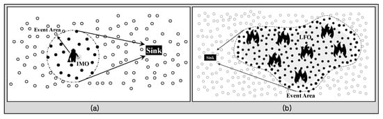
Figure 1.
Data dissemination from an event area to a sink: (a) individual mobile objects (IMOs) vs. (b) large-scale fluid objects (LFOs).
Table 1 represents large-scale and dynamic properties of LFOs by comparing inherent characteristics between IMOs and LFOs. An IMO could be shown as a single coordinate such as (x, y) since its size is very small and invariable. Only several sensor nodes around the IMO sense it and report data to a sink. In IMO monitoring, the sink recognizes the existence and moving trajectory of an IMO with the change of the coordinate from reported data. On the other hand, an LFO is sensed by a large number of sensor nodes since its size is very huge. The LFO is presented by multiple coordinates. In LFO monitoring, the sink recognizes the moving trajectory of an LFO with the alteration of its scope. In consequence, these large-scale and dynamic properties of an LFO require much more seriously the energy efficiency accomplishment to deal with LFO monitoring than the IMO case.

Table 1.
Inherent characteristics of IMOs and FLOs.
3. Energy-Efficient Object Monitoring
In this section, the survey on object monitoring technologies and strategies come up with for IMOs is first fulfilled; then, a technological evolution model with three phases is conducted to evaluate the presence of technological advances for LFO monitoring. This article comes up with a model of technological evolution for IMO and LFO monitoring to reduce communication costs as illustrated in Figure 2: (1) concentration, (2) integration, and (3) abbreviation. Three phases are closely related to communication processes for IMO and LFO monitoring and classified in the perspective what communication process they deal with. In addition, we derive equations for identifying the effectiveness by numerical values. In addition, the experimental comparison of such existing technologies for LFOs is provided to seek advantages of strategies the technologies have followed and leaking points to be broken through.
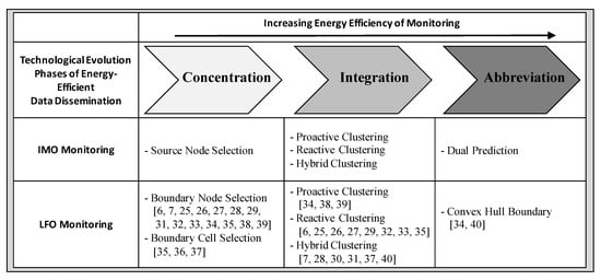
Figure 2.
Survey on energy-efficiency of monitoring for IMOs and LFOs by the technological evolution model.
3.1. Review of IMO Monitoring
Due to energy-constrained sensor nodes, energy efficiency in one of the most important requirements. Studies on energy efficiency typically focus on reducing communication costs since the energy consumption for transmitting and receiving data packets via wireless media is the major factor of battery power consumption of a sensor node [3]. The technological evolution model of IMO monitoring shows key features of all the proposed works in [4,5,12,13,14,15].
IMO monitoring could be naturally achieved by a simple and naïve way that every node sensing the object reports data to a sink as shown in Figure 1a where black dots indicate sensor nodes sensing the IMO (i.e., the tank) and sending its own location with sensing data of the object. The sink could estimate the location and trajectory of the IMO with considering the sensing range of a sensor node. However, this is very expensive as we intuitively know.
The phase I, concentration, prevents duplicated data packet transmissions from all the sensor nodes sensing the IMO to a sink [16]. Therefore, this phase allocates a source node through local decision among the sensor nodes to decide what object is sensed there. The selected source node then interacts with the sink to inform what IMO is detected and where it is. This concentration phase extremely reduces communication cost compared with the naïve idea. Studies for concentration focus on effective cooperation methods among candidates for localized election of a proper sensor node and prevention of other nodes’ reports, so-called the source node selection.
Integration, the phase II, reduces the number of data packets reported along with movement of the IMO [17]. Even though only each source node selected at the concentration phase reports data at a time, concatenated source nodes are continuously generated according to the moving trajectory of the IMO. That is, a number of source nodes are selected within the event areas continuously changing. To reduce this communication cost, studies for integration construct cluster structures; the head of each cluster aggregates IMO detection data from source nodes located within the cluster region; then, the cluster head disseminates aggregated data to a sink. The cluster is established in two means: proactive structuring and reactive structuring. Proactive approaches are more suitable for the application environments with a number of IMOs and rapid mobility of them; in contrast, reactive ones provide efficiency for non-dynamic application environments. Cluster-based data dissemination strategies with signaling to gather data from source nodes and data transmission to a sink are cost-effective since the distance between a cluster head and a sink is usually much further than that between source nodes and a cluster head.
Finally, the phase III, abbreviation, reduces the amount of data to be selected via the concentration and integration phases and reported to a sink [18,19,20,21,22,23,24]. This phase not only decreases the number of data packets but also abbreviates the number of data reporting to a sink. For this phase, dual prediction schemes have been proposed. Every current source node and a sink share the same vector information with speed and direction to define an IMO movement since the movement of an IMO from a point to another point can be defined by a vector. Both of them can predict next locations of an IMO by the information. Then, each current source node compares the prediction result with IMO’s moving behavior. If the prediction is incorrect, the source node reports a new vector information to the sink. Therefore, such dual prediction schemes can reduce the number of data packets as well as times to report.
3.2. Survey of LFO Monitoring
In this subsection, the status and trends of LFO monitoring compared with the technological evolution of IMO monitoring are investigated. Existing schemes are presented and analyzed through the three phrases. First, it could reduce energy consumption by selecting boundary nodes instead of that every detection node reports information. In the next generation, the boundary nodes reduce more energy consumption by integrating reporting information through clustering among them. Then, it significantly reduces the number of boundary reports by utilizing dual prediction. It predicts a shape of LFO and with the correct prediction the reporting can be skipped. During the designing of object monitoring, all the three stages need to be addressed, and the effectiveness of object monitoring E could be defined as
where is a positive integer representing the number of source nodes which detect the object, and is a non-negative integer representing the reported number of source nodes by the network after stage. In Equation (1), the effectiveness of object monitoring E satisfies .
3.2.1. Phase I: Concentration
In LFO monitoring, candidates of source nodes considered in IMO monitoring can be located near the boundary of an LFO, not all nodes sensing the LFO as shown in Figure 1b. Monitoring schemes first distinguish these candidates and then choose source nodes, called boundary nodes (BNs), among the candidates. In other words, concentration for LFO monitoring means selection of BNs. This phase could be represented as
where is a non-negative integer representing the number of sensor nodes which will be reported to proceed to the next phase, is a collection of design parameters to be determined by the choice of concentration phase, and the process of concentration is abstracted as a black box function with respect to the detected sensor nodes and design parameters of concentration . In Equation (2), , which means some source nodes are concentrated to perform further actions after the concentration phase.
DCS [25] and COBOM [26] provide a mechanism to suppress sensor nodes located near the center of an LFO since LFO monitoring means tracking boundary shape alteration of it. In DCS, if a sensor node senses the LFO and one or more neighbors do not sense the LFO, the sensor node becomes a BN. In COBOM, if a sensor node has one or more neighbors whose sensing states are different from itself, the sensor node becomes a BN. In other words, DCS elects BNs only among nodes that sense the LFO whereas nodes that do not sense LFO could be BNs in COBOM. Due to this difference of BN election algorithms, the number of BNs in DCS is a little less than COBOM. EUCOW [27] theoretically reduces the half of the number of BNs in comparison with COBOM. EUCOW divides BN candidates into two groups: BN candidates located in “IN” range and BN candidates located in “OUT” range. Nodes located in “IN” range are suppressed when the LFO expands; whereas nodes located in “OUT” range are suppressed when LFO shrinks. EUCOW also shows that they do not lose quality of LFO detection. DeGas [7] and GLDS [28] also select multiple BNs by collaboration with inner boundary nodes (IBNs) and outer boundary nodes (OBNs). TPE-FTED [29] conducts pattern matching for sensor nodes to identify fault-tolerant event regions. TG-COD [30] proposes the geographic-cell-based boundary detection. It detects the boundary shape of an LFO via an absolute criterion while the other works exploit relative ones such as hop counts and deployed node density. TG-COD establishes fine-grained grid cells referring to geographical coordinates, and then it decides whether a geographical cell is the boundary cell or not by the ratio of sensing nodes and non-sensing nodes within the cell. The other studies for LFO monitoring mainly apply the BN election algorithm of DCS and focus on other phases.
TGM-COT [31], BRTCO [6], PM-COT [32] and BTS-COT [33] construct their own structure (grid-based, Delaunay triangulation-based, Tree-based). TGM-COT divides the network into grids for object detection. By the trangular mesh, the BRTCO and PM-COT nodes located outside the event region determine collaboratively the line of objects. BTS-CTO makes a full binary tree structure to achieve the boundary area mapping. However, they suffer from overhead of the node-level structure management owing to a number of sensor nodes in the field.
3.2.2. Phase II: Integration
Technologies for integration in IMO monitoring concentrate on temporal aggregation since they do not need to integrate a coordinate that a source node reports as a point at a certain time. However, the integration for LFO monitoring should take into account spatial aggregation as well as temporal aggregation because the boundary information of an LFO is composed of many coordinates. Effectiveness and importance of integration are much higher than that of IMO monitoring. Existing studies for LFO monitoring aggregate data to be reported through diverse clustering techniques. This phase could be represented as
where is a non-negative integer representing the number of sensor nodes which will be reported to proceed to the next phase, is a collection of design parameters to be determined by the choice of integration factors, and the process of integration is abstracted as a black box function with respect to the selected source nodes after the last concentration phase and design parameters of integration . In Equation (3), , which means some source nodes are integrated to perform further actions after the integration phase.
After BN election process, DCS constructs reactive clusters, called dynamic cluster structure (DCS), composed of a certain number of BNs for data aggregation as shown in Figure 3a. Every cluster then elects a cluster head among its BNs. DCS could reduce the number of data packets reported to a sink since the cluster head gathers data from BNs and transmits the aggregated data. As a boundary shape of an LFO is altered, new BNs are elected frequently; then, DCS reconstructs clusters and re-elects cluster heads. Dynamic clustering schemes, therefore, consume a large amount of energy for frequent cluster reconstruction.
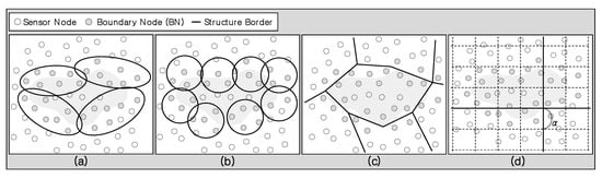
Figure 3.
Integration strategies: (a) reactive cluster, (b) reactive one-hop cluster, (c) proactive cluster, and (d) hybrid cluster.
COBOM [26], EUCOW [34], PRECO [35], and FPOD [36] establish reactive one-hop clusters over one-hop neighbor BNs as shown in Figure 3b. Each cluster head collects data from one-hop neighbor BNs and reports the aggregated data to the sink. Even though reactive one-hop clustering schemes also reconstruct clusters in response of LFO’s alteration, the cost of communication for such cluster reconstruction is relatively very small since one-hop cluster could be constructed by a few one-hop message exchanges. However, the effect of data aggregation is insufficient due to few BNs within a one-hop cluster.
CODA [34] and BFA [37] initially and proactively establish static clusters composed of all sensor nodes on a whole sensor field and each cluster elects a cluster head among sensor nodes located in the cluster. Figure 3c illustrates these proactive clusters. When an LFO appears, the cluster head gathers data from BNs located in the cluster and reports the aggregated data to the sink. Static clustering schemes do not need to reconstruct clusters since clusters are composed of static members not BNs. Although BNs are changed in response of LFO’s alteration, new BNs already know their own clusters and the cluster heads. Static clustering schemes however consume more energy for clusters construction and maintenance than dynamic clustering schemes. Static clustering schemes construct clusters on a whole sensor field whether an LFO appears or not, whereas dynamic clustering schemes construct clusters only near the boundary of the LFO.
TG-COD [30] and TGM-COT [31] rely on a two-tier grid structure which considers both proactive and reactive approaches. This hybrid cluster in Figure 3d represents taking both advantages of proactive and reactive approaches, so that they could support fast diffusion of an LFO with high energy efficiency for structure construction. It first proactively constructs coarse-grained grid cells by referring at a geographical coordinate. Then, when an LFO happens nearby a coarse-grained call, the cell establishes fine-grained grid cells within itself. The grid cells are generated with values as geographical distances, e.g., for fine-grained cells ‘’.
GAS [38] and COTS [39] similarly construct proactive virtual clusters which means a grid structure calculated with only location information. Each sensor node could know its own cluster by calculation with its own location, a reference point, and a cluster size without communication among sensor nodes. Cluster heads are also elected by calculation. Therefore, TG-COD, TGM-COT, GAS, and COTS do not suffer from communication overhead for cluster construction and maintenance. Figure 4 and Table 2 summarize the energy efficiency of such integration techniques.
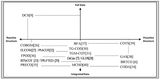
Figure 4.
Comparison of technologies for integration levels, structure types, and communication overhead. Integration levels and communication overhead are represented between full data (all boundary information) and integrated data.
Table 2.
Comparison of technologies in terms of clustering overhead.
3.2.3. Phase III: Abbreviation
Dual prediction techniques that are proposed for abbreviation in IMO monitoring are not studied yet in LFO monitoring. Dual prediction for LFO monitoring is much more complex than that for IMO monitoring since it has to predict the next boundary shape not the next point. For example, if the present boundary is composed of 30 coordinates, the next boundary might be composed of 35 coordinates and each part of the boundary has different vectors due to the dynamic property of an LFO. This phase could be represented as
where is a non-negative integer representing the number of sensor nodes which will be finally reported, is a collection of design parameters to be determined by the choice of abbreviation factors, and the process of abbreviation is abstracted as a black box function with respect to the selected source nodes after the last abbreviation phase NI and design parameters of integration . In Equation (4), , which means some source nodes after the last phase are abbreviated to be reported after the abbreviation phase.
Unlike IMO monitoring, CODA for LFO monitoring proposes a data abbreviation scheme using geometric modeling thanks to the large-scale property of an LFO. CODA applies the convex hull algorithm for abbreviation to collect data in the integration phase. Cluster heads could decide the smallest set of coordinates among collected coordinates by the convex hull algorithm and reduce the amount of data to be reported. However, an LFO typically has concave and irregular shapes but the convex hull algorithm returns only the convex set of BN locations. CODA consequently achieves data abbreviation but the qualitative loss of LFO monitoring is occurred.
MCHD [40] proposed a novel mechanism to reduce the number of nodes participating in transmission based on convex-hull. The mechanism resolves the shortage of dealing with concave and irregular shapes by convex identification process. In case of a non-convex shape LFO, MCHD conducts the recovery process to fill only the misrecognized section. The mechanism takes both low communication cost and high detection reliability of LFO.
3.3. Experimental Study
LFO monitoring schemes are evaluated for detection quality and energy efficiency. Experiments are conducted by QualNet simulator with 400 sensor nodes running with IEEE 802.15.4, deployed in a 200 m × 200 m squarearea. An LFO with a width of 20 m initially exists and contentiously enlarges in the second and third experiments. Each simulation run lasts for 200 s, and a source generates one data packet per second. Each data packet has 64 bytes. Transmitting, receiving, and idling power consumption rates of the sensors are 21 mW, 15 mW, and 0.03 mW, respectively. The parameters are chosen in reference to the MICA specification. Firstly, the correlation between quality of recognized shapes of an LFO and quantity of data packets delivered to a sink is provided. Then, the total communication costs are explained to check impacts of the LFO size and node density. The studies which consider the sleep mode of sensor nodes are not compared together since they are extremely focused on only reduction of energy consumption with excluding data dissemination processes to a sink.
The experiment uses a kidney bean shape of an LFO as a concave one. The LFO is initiated with a width of 20 m and a height of 10 m at center (50, 50). Figure 5 illustrates detection results about the LFO. DCS selects BNs and reactive clusters of BNs are constructed. Integration of DCS is simple aggregation by heads of clusters, so the number of delivered data at a sink is large. In COBOM, one-hop clusters are established and heads of the clusters disseminate only one datum point to a sink. Namely, the number of clusters are larger than DCS, but the number of delivered data is smaller than that. EUCOW has the goal to reduce the number of BNs considering LFO’s diffusion direction. Accordingly, it decides only the approximate shape of the LFO with the smaller number of clusters than COBOM. In CODA, headers of proactive clusters gather location information of all sensor nodes which detect the continuous object; however, CODA is dependent on the convex hull algorithm so that it determines concave shapes into convex ones. Thus, CODA cannot detect reliably the concave objects. On the other hand, TG-COD chooses fine-grained grid cells as the boundary cells over coarse-grained grid cells. The drawing of LFO’s border by the boundary cells follows grid shapes although TG-COD has many advantages against LFO alteration and node density, so here this article does not compare it with others’ detection results via graphs.
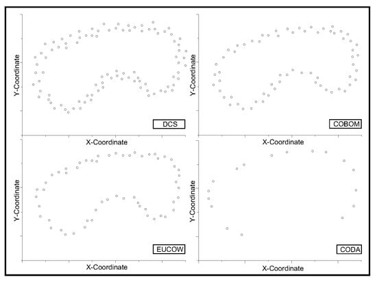
Figure 5.
Experimental results for quality vs. quantity.
Figure 6 shows the effect of the different size of an LFO in terms of energy consumption. Energy consumption is depending on the clustering cost and the data dissemination cost. Each scheme has two results in cases that the width of the LFO grows from 20 m to 40 m and the width of it enlarges from 20 m to 60 m. DCS, COBOM, and EUCOW consume more energy for clustering than CODA and TG-COD since they reconstruct clusters along with alteration of the LFO. COBOM and EUCOW have lower values than DCS since the one-hop cluster construction cost is relatively smaller than multi-hop clustering. Clustering costs of DCS, COBOM, and EUCOW are also not decoupled from the size of the LFO and spend more energy due to increasing the LFO size. Clustering costs of CODA and TG-COD, however, are not affected by the size. These results are caused since DCS, COBOM, and EUCOW reactively construct structures with BNs whereas CODA and TG-COD proactively construct structures regardless of LFO’s alteration. Dissemination costs of DCS, CODA, and TG-COD have similar results because the effect of integration is similar if their cluster sizes are similar. However, COBOM and DEMOCO consume more energy for dissemination because of smaller cluster sizes. The dissemination cost could not be decoupled from the size of LFO since the amount of reporting data is naturally proportional to the size of the LFO.
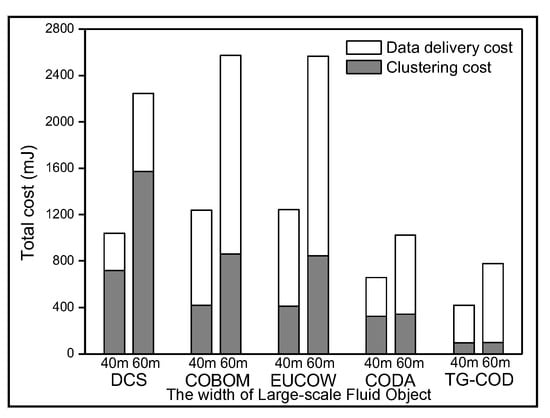
Figure 6.
Experimental results for cost with different LFO sizes.
Figure 7 represents the impact of the different node density. Each scheme has two results in cases that the number of sensor nodes is 400 and 800. Clustering costs of DCS, COBOM, and EUCOW are not decoupled from the node density as well as from the size of the LFO since more sensor nodes participate in cluster construction along with increase of the node density. DCS constructs more clusters since it decides the size of a cluster on the basis of the number of BNs. Clustering cost of CODA is also not decoupled from the node density unlike the size of the LFO and consumes more energy. TG-COD is not affected by the node density. This result is caused by that CODA construct clusters through communication between sensor nodes whereas TG-COD constructs virtual clusters which refers to an independent coordinate. Data dissemination cost of DCS is not decoupled from the node density since it constructs more clusters and the effect of integration is reduced. COBOM and EUCOW consumes more energy for data dissemination than CODA and TG-COD due to the restricted clustering but they are decoupled from the node density. Decoupling of COBOM, EUCOW, CODA, and TG-COD in terms of data dissemination cost is caused by that the sizes of their clusters are not changed by the node density.
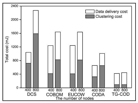
Figure 7.
Experimental results for cost with different node densities.
Figure 8 shows the number of packet transmissions by the impact of transmission range irregularity. Transmission range irregularity means non-isotropic form of transmission range due to the radio feature. We assumed the irregularity follows Radio Irregularity Model (RIM) with Degree of Irregularity (DOI) = 0.003. This phenomenon makes neighbor information asymmetric to each other. In this case, one side transmits packets to its neighbor and expects relaying packet or acknowledgment, but the neighbor might not have reachability. Eventually, it might be regarded as transmission error and causes re-transmission. DCS, COBOM, and EUCOW face this problem more frequently due to reconstructing clusters requiring communications with each other. On the other hand, proactive schemes, CODA and TG-COD, are less affected.
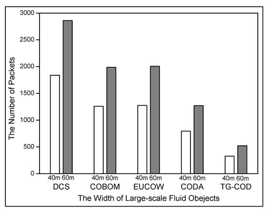
Figure 8.
Experimental results for cost with transmission range irregularity.
4. Future Research Challenges
A survey was conducted on the latest LFO monitoring technologies, and findings were analyzed and evaluated with respect to lack of them in three technological evolution phases. Namely, compared with IMO monitoring, LFO monitoring still has many rooms to be broken through as follows: (1) concentration decoupling with node density that seriously harms energy efficiency, (2) integration not only decoupling with network structure for energy-efficient structure maintenance but also trading off the size of a cluster and the level of aggregation, and (3) abbreviation dealing with the quality of LFO detection and the quantity of delivered data as well as supporting irregularity of dynamic scopes of an LFO. Based on the new model with phases of concentration, integration, and abbreviation, the effectiveness of LFO monitoring in Equation (1) can be rewritten as
using Equations (2)–(4). This equation represents the new effectiveness model as a generalized abstraction. Instantiation could vary depending on selection of black box functions and the parameters set. Though explicit definition of functions and parameters is not feasible in an instant, some research challenges regarding to the three phases can be identified based on the existing systems mentioned in this article.
Furthermore, monitoring of LFOs should be fulfilled with high quality for not only suppression of them but also evacuation recommendation of people since LFOs could cause more serious problems to people who live nearby LFOs. Namely, LFO monitoring needs to be progressively improved with high reliability of detection and tracking and sustainability of monitoring infrastructure. For these goals, LFO monitoring should take into account big data analytics technologies in IoT environments including clouds, so-called IoT analytics. To provide high quality of user experience, new information and analytics approaches using user smartphones such as activity sensing [9] should be exploited. In addition, sensor nodes are prone to battery exhaustion, so harvesting technologies [8] should be adopted into sensor nodes for sustainable monitoring. Finally, cutting-edge localization technologies such as Bluetooth low energy-based beaconing [9] should be cooperated with LFO monitoring systems since the monitoring information is mainly the location information of borders of LFOs.
5. Conclusions
The shape of an LFO is dynamically changed and relatively much more unpredictable than that of an IMO since LFOs are typically sensitive against natural effects such as wind, temperature, and geographical features. Firstly, this article defined an analytical model of technological evolution for energy-efficient monitoring, and then it was employed to analyze LFO monitoring schemes. In addition, experiment studies by three different scenarios of detection quality and energy efficiency supported finding challenges from the survey and analysis on the schemes. Finally, this article addressed not only such challenges in communication perspective with the defined model, but also important interoperable points with state-of-the-art technologies as future research challenges.
Author Contributions
Y.Y. contributed to investigation and original draft writing. E.L. contributed to conceptualization and validation. S.O. contributed to resources, supervision, and review/editing. All authors have read and agreed to the published version of the manuscript.
Funding
This research received no external funding.
Acknowledgments
This work was supported by the National Research Foundation of Korea (NRF) grant funded by the Korea government (MSIT) (No. NRF-2020R1C1C1010692).
Conflicts of Interest
The authors declare no conflict of interest.
References
- Liu, J.; Li, Y.; Chen, M.; Dong, W.; Jin, D. Software-defined internet of things for smart urban sensing. IEEE Commun. Mag. 2015, 53, 55–63. [Google Scholar] [CrossRef]
- Rashid, B.; Rehmani, M.H. Applications of wireless sensor networks for urban areas: A survey. J. Netw. Comput. Appl. 2016, 60, 192–219. [Google Scholar]
- Akyildiz, I.F.; Su, W.; Sankarasubramaniam, Y.; Cayirci, E. A survey on sensor networks. IEEE Commun. Mag. 2002, 40, 102–114. [Google Scholar] [CrossRef]
- Li, D.; Wong, K.D.; Hu, Y.H.; Sayeed, A.M. Detection, classification, and tracking of targets. IEEE Signal Process. Mag. 2002, 19, 17–29. [Google Scholar]
- Bhatti, S.; Xu, J. Survey of target tracking protocols using wireless sensor network. In Proceedings of the International Conference on Wireless and Mobile Communications, Cannes, France, 23–29 August 2009; pp. 110–115. [Google Scholar]
- Han, G.; Shen, J.; Liu, L.; Shu, L. BRTCO: A novel boundary recognition and tracking algorithm for continuous objects in wireless sensor networks. IEEE Syst. J. 2016, 12, 2056–2065. [Google Scholar] [CrossRef]
- Shu, L.; Mukherjee, M.; Wu, X. Toxic gas boundary area detection in large-scale petrochemical plants with industrial wireless sensor networks. IEEE Commun. Mag. 2016, 54, 22–28. [Google Scholar] [CrossRef]
- Zheng, J.; Cai, Y.; Shen, X.; Zheng, Z.; Yang, W. Green energy optimization in energy harvesting wireless sensor networks. IEEE Commun. Mag. 2015, 53, 150–157. [Google Scholar] [CrossRef]
- Vigneshwaran, S.; Sen, S.; Misra, A.; Chakraborti, S.; Balan, R.K. Using infrastructure-provided context filters for efficient fine-grained activity sensing. In Proceedings of the IEEE international conference on pervasive computing and communications (PerCom), St. Louis, MO, USA, 23–27 March 2015; pp. 87–94. [Google Scholar]
- Hussein, D.; Park, S.; Han, S.N.; Crespi, N. Dynamic social structure of things: A contextual approach in CPSS. IEEE Internet Comput. 2015, 19, 12–20. [Google Scholar] [CrossRef]
- Han, S.N.; Park, S.; Lee, G.M.; Crespi, N. Extending the devices profile for web services standard using a REST proxy. IEEE Internet Comput. 2014, 19, 10–17. [Google Scholar] [CrossRef]
- Feng, J.; Zhao, H. Energy-balanced multisensory scheduling for target tracking in wireless sensor networks. Sensors 2018, 18, 3585. [Google Scholar] [CrossRef]
- Shen, J.; Yin, M.; Luo, J.A.; Wang, Z.B.; Wang, Z.; Li, Z.H. An Energy Efficient Synchronization Protocol for Target Tracking in Wireless Sensor Array Networks. Sensors 2019, 19, 1367. [Google Scholar] [CrossRef]
- Liu, M.; Zhang, D.; Zhang, S.; Zhang, Q. Node depth adjustment based target tracking in UWSNs using improved harmony search. Sensors 2017, 17, 2807. [Google Scholar] [CrossRef] [PubMed]
- Souza, É.L.; Nakamura, E.F.; Pazzi, R.W. Target tracking for sensor networks: A survey. ACM Comput. Surv. (CSUR) 2016, 49, 1–31. [Google Scholar] [CrossRef]
- Shorey, R.; Ananda, A.; Chan, M.C.; Ooi, W.T. Mobile, Wireless, and Sensor Networks: Technology, Applications, and Future Directions; John Wiley & Sons: Hoboken, NJ, USA, 2006. [Google Scholar]
- Tsai, H.W.; Chu, C.P.; Chen, T.S. Mobile object tracking in wireless sensor networks. Comput. Commun. 2007, 30, 1811–1825. [Google Scholar] [CrossRef]
- Xue, L.; Liu, Z.; Guan, X. Prediction-based protocol for mobile target tracking in wireless sensor networks. J. Syst. Eng. Electron. 2011, 22, 347–352. [Google Scholar] [CrossRef]
- Wang, G.; Wang, H.; Cao, J.; Guo, M. Energy-efficient dual prediction-based data gathering for environmental monitoring applications. In Proceedings of the IEEE Wireless Communications and Networking Conference, Kowloon, China, 11–15 March 2007; pp. 3513–3518. [Google Scholar]
- Xu, Y.; Winter, J.; Lee, W.C. Prediction-based strategies for energy saving in object tracking sensor networks. In Proceedings of the IEEE International Conference on Mobile Data Management, Berkeley, CA, USA, 19–22 January 2004; pp. 346–357. [Google Scholar]
- Xu, Y.; Winter, J.; Lee, W.C. Dual prediction-based reporting for object tracking sensor networks. In Proceedings of the First Annual International Conference on Mobile and Ubiquitous Systems: Networking and Services (MOBIQUITOUS), Boston, MA, USA, 26 August 2004; pp. 154–163. [Google Scholar]
- Wang, Z.; Li, H.; Shen, X.; Sun, X.; Wang, Z. Tracking and predicting moving targets in hierarchical sensor networks. In Proceedings of the IEEE International Conference on Networking, Sensing and Control, Sanya, China, 6–8 April 2008; pp. 1169–1173. [Google Scholar]
- Bhuiyan, M.; Wang, G.j.; Zhang, L.; Peng, Y. Prediction-based energy-efficient target tracking protocol in wireless sensor networks. J. Cent. South Univ. Technol. 2010, 17, 340–348. [Google Scholar] [CrossRef]
- Deldar, F.; Yaghmaee, M.H. Designing an energy efficient prediction-based algorithm for target tracking in wireless sensor networks. In Proceedings of the International Conference on Wireless Communications and Signal Processing (WCSP), Nanjing, China, 9–11 November 2011; pp. 1–6. [Google Scholar]
- Ji, X.; Zha, H.; Metzner, J.; Kesidis, G. Dynamic cluster structure for object detection and tracking in wireless ad-hoc sensor networks. In Proceedings of the IEEE International Conference on Communications, Paris, France, 20–24 June 2004; Volume 7, pp. 3807–3811. [Google Scholar]
- Zhong, C.; Worboys, M. Continuous contour mapping in sensor networks. In Proceedings of the IEEE Consumer Communications and Networking Conference, Las Vegas, NV, USA, 10–12 January 2008; pp. 152–156. [Google Scholar]
- Chen, J.; Matsumoto, M. EUCOW: Energy-efficient boundary monitoring for unsmoothed continuous objects in wireless sensor network. In Proceedings of the IEEE International Conference on Mobile Adhoc and Sensor Systems, Macau, China, 12–15 October 2009; pp. 906–911. [Google Scholar]
- Shu, L.; Chen, Y.; Sun, Z.; Tong, F.; Mukherjee, M. Detecting the dangerous area of toxic gases with wireless sensor networks. IEEE Trans. Emerg. Top. Comput. 2017, 8, 137–147. [Google Scholar] [CrossRef]
- Liu, L.; Han, G.; He, Y.; Jiang, J. Fault-tolerant event region detection on trajectory pattern extraction for industrial wireless sensor networks. IEEE Trans. Ind. Informatics 2019, 16, 2072–2080. [Google Scholar] [CrossRef]
- Park, S.; Park, H.; Lee, E.; Kim, S.H. Reliable and flexible detection of large-scale phenomena on wireless sensor networks. IEEE Commun. Lett. 2012, 16, 933–936. [Google Scholar] [CrossRef]
- Han, G.; Shen, J.; Liu, L.; Qian, A.; Shu, L. TGM-COT: Energy-efficient continuous object tracking scheme with two-layer grid model in wireless sensor networks. Pers. Ubiquitous Comput. 2016, 20, 349–359. [Google Scholar] [CrossRef]
- Liu, L.; Han, G.; Shen, J.; Zhang, W.; Liu, Y. Diffusion distance-based predictive tracking for continuous objects in industrial wireless sensor networks. Mob. Netw. Appl. 2019, 24, 971–982. [Google Scholar] [CrossRef]
- Liu, L.; Han, G.; Xu, Z.; Jiang, J.; Shu, L.; Martinez-Garcia, M. Boundary tracking of continuous objects based on binary tree structured SVM for industrial wireless sensor networks. IEEE Trans. Mob. Comput. 2020. [Google Scholar] [CrossRef]
- Chang, W.R.; Lin, H.T.; Cheng, Z.Z. CODA: A continuous object detection and tracking algorithm for wireless ad hoc sensor networks. In Proceedings of the IEEE Consumer Communications and Networking Conference, Las Vegas, NV, USA, 10–12 January 2008; pp. 168–174. [Google Scholar]
- Park, S.; Hong, S.W.; Lee, E.; Kim, S.H.; Crespi, N. Large-scale mobile phenomena monitoring with energy-efficiency in wireless sensor networks. Comput. Netw. 2015, 81, 116–135. [Google Scholar] [CrossRef]
- Imran, S.; Ko, Y.B. A continuous object boundary detection and tracking scheme for failure-prone sensor networks. Sensors 2017, 17, 361. [Google Scholar] [CrossRef]
- Ping, H.; Zhou, Z.; Shi, Z.; Rahman, T. Accurate and energy-efficient boundary detection of continuous objects in duty-cycled wireless sensor networks. Pers. Ubiquitous Comput. 2018, 22, 597–613. [Google Scholar] [CrossRef]
- Park, H.; Oh, S.; Lee, E.; Park, S.; Kim, S.H.; Lee, W. Selective wakeup discipline for continuous object tracking in grid-based wireless sensor networks. In Proceedings of the IEEE Wireless Communications and Networking Conference (WCNC), Paris, France, 1–4 April 2012; pp. 2179–2184. [Google Scholar]
- Oh, S.; Cho, H.; Kim, S.H.; Lee, W.; Lee, E. Continuous object tracking protocol with selective wakeup based on practical boundary prediction in wireless sensor networks. Comput. Netw. 2019, 162, 106854. [Google Scholar] [CrossRef]
- Oh, S.; Lee, J.; Park, S. Energy efficient and accurate monitoring of large-scale diffusive objects in internet of things. IEEE Commun. Lett. 2016, 21, 612–615. [Google Scholar] [CrossRef]


Publisher’s Note: MDPI stays neutral with regard to jurisdictional claims in published maps and institutional affiliations. |
© 2021 by the authors. Licensee MDPI, Basel, Switzerland. This article is an open access article distributed under the terms and conditions of the Creative Commons Attribution (CC BY) license (http://creativecommons.org/licenses/by/4.0/).