1. Introduction
In automotive field, the full play performance of active safety system depends on the accurate multi-information including road conditions, vehicle parameters and vehicle states [
1,
2,
3,
4]. Currently, an economical way to obtain these kinds of information is a soft-sensing approach. However, most of the reported approaches can only be applied under a simplex driving scenario, where the road is flat [
5] or the vehicle mass is constant [
6]. Actually, due to terrain constraints or design need, the assumption of horizontal road cannot be met, and its mass may vary in several hundred kilograms as a vehicle is full or empty. In addition, there are coupling relationships in the acquisition process of road conditions, vehicle coefficients and vehicle states [
2,
7,
8,
9]. It is helpful to improve the soft-sensing accuracy by integrating multiple information. Hence, it is necessary to study effective joint soft-sensing approach for multi-information.
The traditional joint soft-sensing approaches in the automotive field can be categorized into centralized, reinforced and distributed structures. For the centralized structure, a unified model is utilized to get different information synchronously, which is simple and there is less redundancy. In allusion to road conditions and vehicle parameters, such as the time-varying road slope and vehicle mass, a modified RLS algorithm with multiple forgetting-factors was proposed [
10]. In addition, an observer-based scheme with sliding-mode term was developed using onboard sensor signals [
3]. Although these above two methods have good accuracy, the road slope results reveal the defect of time delay. However, the centralized structure, in exceptional cases, may present poor accuracy performance or even divergence. Addressing this issue, the reinforced structure was adopted by means of an additional part to enhance the stability of soft-sensing results. For instance, the EKF and RLS were integrated to obtain the road slope and vehicle mass [
11], which provided higher accuracy and faster convergence. In another study, the RLS with multiple factors and EKF are, respectively, adopted in two steps of an estimator, which shows great accuracy and robustness in vehicle road test [
12]. Similarly, a two-stage estimation strategy was proposed to determine the road slope and mass of heavy-duty vehicle [
9]. However, the design is too complicated and difficult to be applied in practice.
As compared with the centralized structure, the reinforced one has better performance on accuracy and convergence. However, the real-time performance of the latter is dissatisfactory due to its complex construction. As an alternative, the distributed structure employs independent modules to obtain different information, which is beneficial to balance the accuracy and calculation burden. For the module design in the distributed structure, recursive algorithms gain widespread attention, such as the KF [
2], observer-based method [
4], and RLS [
13]. In addition, Hong et al. [
14] used three UKFs to obtain the inertial parameters and vehicle states, respectively. However, the complication limits its further generalization. For eliminating the influence of vehicle parameters on vehicle states, Wenzel et al. [
8] utilized a DEKF technique, which was primarily proposed by Wan and Nelson [
15]. However, this solution does not perform well under ramp road conditions. Moreover, adaptive high-order sliding-mode observer and strong tracking filter were adopted to estimate the information of force, speed and angle for electric vehicle [
16]. However, the influence of time-variant noise was not fully considered in its results. Viehweger et al. [
17] analyzed four estimation methods about vehicle state and tire force, which shows that the performance of the suboptimal-second order sliding mode and EKF-based method is better in the slow track condition, and the error of the purely linear and EKF-based method is lower in the fast track condition. Considering the complexity of the vehicle’s COG in three-dimensional space, a distributed structure-based approach synthesized both vehicle longitudinal and lateral motion, which effectively improves its behaviour [
18].
There are also some deficiencies in the traditional joint soft-sensing approaches, such as the time delay of some information and the compatibility for time-variant noise. To lower the time delay, a short-time linear quadratic technique was proposed for the achievement of road slope [
19]. However, it is not a good choice because of its complexity. As the consideration of time-variant noise, Berntorp et al. [
7,
20] adopted a PF framework. However, the calculation of vast particles results in poor real-time performance.
In addition, the response results of the soft-sensing are affected by many factors related to the driver, roadway geometry, environment, vehicle, and so on. It is difficult to consider the interference of all factors in scientific research, or it may lead to a problem called "observational heterogeneity" (the unobservable or unavailable factors in the effect of results that are unknown) [
21,
22]. If this problem is ignored, the erroneous inferences and predictions that may occur due to the model are misspecified and the estimated parameters are biased [
23,
24]. Some methods are proposed to deal with it, such as the random parameters method, finite mixtures (latent classes) method and their combination [
25,
26]. Recently, artificial neural networks have also been used to solve the observational heterogeneity [
27].
In case the road conditions change and the vehicle parameters are unknown, it is an important requirement for the automobile development to ensure the effectiveness of soft-sensing. On this basis, an urgent need is to continuously improve the performance of measurement results in terms of accuracy, robustness, time delay, and so on. The motivation of this study is to acquire the vehicle required information even under diverse vehicle driving scenarios. In this paper, a joint soft-sensing strategy is developed to obtain accurate multi-information based on the distributed structure. The information interaction in this strategy is realized according to the coupling relationship among the vehicle state, road slope and vehicle mass. The time-variant noise problem in the vehicle states estimation is adaptively disposed by a VBACKF. To alleviate the time delay of road slope, a slope prediction model is derived to replace the classical road slope model and the corresponding observer is designed with a cubic term. Finally, the contrast experiment is implemented to evaluate the performance of the proposed strategy.
The rest of this paper is organized as follows. The overview of the strategy is presented in
Section 2. The vehicle dynamics model involving road slope is introduced in
Section 3.
Section 4,
Section 5 and
Section 6 show the details on how to achieve the vehicle states, road slope and vehicle mass in turn. The experiment is described in
Section 7, and followed by the conclusions in
Section 8.
2. Joint Soft-Sensing Strategy
Aiming at the problem that the application scenario of most soft-sensing approaches is simplex, a joint soft-sensing strategy is proposed. As shown in
Figure 1, this strategy mainly consists of three modules: vehicle state estimation, road slope observation and vehicle mass determination. To realize the application of the non-horizontal road scenario, firstly, a vehicle model considering road slope is established. Based on this model, a VBACKF is utilized in the vehicle state estimation module to deal with the time-variant noise via two steps: time update and variational measurement update. In the road slope observation module, a novel slope prediction model and a cubic observer are used to design an observer, which is expected to reduce the time delay. According to the variation character of vehicle mass, a FFRLS algorithm is employed to determine vehicle mass. In addition, the data preprocessing and the threshold judgment steps are added to eliminate the unreliable input data.
Through this joint soft-sensing strategy, the vehicle state
, road slope
and vehicle mass
are finally obtained, as shown in
Figure 1. (Throughout this paper, the superscript “∧” means the obtained signals from the strategy.) These data can be used not only to serve as the output, but also to apply to implement the information interaction within the strategy. The vehicle state
is adaptively estimated based on the observed road slope from the second module, the determined vehicle mass from the third module and the signals acquired from onboard sensors, such as the steering wheel angle, wheel rotational velocity, vehicle acceleration, and yaw rate. With the estimated value
, some onboard sensor signals are also provided for the observation of the road slope, such as the acceleration and yaw rate. Ultimately, by means of the real-time information including the estimated vehicle state
and observed road slope
, the vehicle mass
is determined according to the information from the vehicle system, i.e., the engine torque, transmission ratio, and braking torque. For this strategy, only the driver’s operation is treated as system input, and there is not any other special sensor equipped.
3. Vehicle Dynamics Modelling
Considering that a vehicle’s dynamics characteristic is closely related to road conditions, a nonlinear vehicle model is presented with road slope
(see
Figure 2), where COG is the center of gravity, the relationship between the steering wheel angle
and the steering angle of front wheels
is assumed as
,
is the steering gear ratio of the steering system. The vehicle’s longitudinal, lateral and yaw vehicle motions can be described as
where
is the longitudinal velocity,
is the lateral velocity,
r is the yaw rate,
is the moment of the inertia around the
z-axis,
is the longitudinal acceleration,
is the lateral acceleration,
is the yaw moment.
Due to the influence of road slope, the vehicle’s gravity is decomposed into two components:
along the
x-axis and
along the
z-axis. The first component mainly affects the vehicle’s longitudinal force
where
m is the vehicle mass,
g is the gravitational acceleration,
and
are the longitudinal and lateral tire forces of each wheel, the subscripts 1, 2, 3, 4 represent the left front, right front, left rear and right rear tire,
is the aerodynamic drag coefficient,
A is the frontal area of the vehicle,
is the air density.
In addition,
,
can be expressed as
where
and
are the distances from the COG to front and rear axles,
and
are the front and rear track width.
As a result of the component along the
z-axis, the vertical tire forces on each tire
are
where
h is the height of COG.
The wheel side angle
, wheel slip rate
and forward wheel speed
are presented as
where
is the wheel rotational speed,
is the wheel radius.
In this study, we use the Dugoff tire model [
28] to generate the longitudinal and lateral tire forces, because of its good behavior in online computation and accuracy. As follows
where
and
are the longitudinal and lateral wheel stiffnesses.
is the model parameter,
is the road adhesion coefficient.
4. Vehicle State Estimation
On the basis of the vehicle model in
Figure 2, the continuous state space for vehicle state estimation can be written as follows
where
are the process and measurement functions,
is the state vector, the input vector
, the measurement vector
consists of the longitudinal acceleration, lateral acceleration and yaw rate,
and
are the process and measurement noises with the covariance matrices
and
.
In the framework of the CKF, the measurement noise is assumed as Gaussian white noise with constant mean and covariance [
29]. This signifies that it is indispensable for good soft-sensing results to get the feature of measurement noise covariance [
30]. However, time-variant noise covariance is a prevalent problem in practical application. It even has been one of the main reasons that lead to the divergence of estimation result [
20,
31]. In this study, the VBACKF is employed to handle the issue of time-variant noise.
Firstly, the conjugate prior distributions need to be selected for the measurement noise covariance matrix
at time
k since the conjugacy can guarantee that the posterior distribution is of the same functional form as the prior distribution [
30]. In Bayesian statistics, the IW distribution is usually used as the conjugate prior for the covariance matrix [
32], i.e.,
. where
is the inverse scale matrix representing a symmetric positive definite matrix with the dimension of
,
is the degrees of freedom parameter, and the noise covariance matrix
is represented by the mean of the IW distribution
Based on the mean field theory, the joint probability density function
of the vehicle state
and measurement noise
is expressed as the product of their approximate probability density function
and
The approximate solutions of the
and
can be obtained by minimizing the KLD
Based on the VBACKF algorithm, the vehicle state estimation module contains two steps: time update and variational measurement update, as shown in
Figure 3. The time update realizes the prediction of the vehicle state vector
and its covariance matrix
through the cubature points. Subsequently, the time-variant measurement noise covariance matrix
is also predicted out in this part. For another part, the vehicle state vector
is updated not only through the cubature points, but also by means of the variational iteration. Meanwhile, the time-variant measurement noise covariance matrix
is adaptively characterized by use of the variational iteration as well. It should be noticed that the number
N is an important parameter used to balance the accuracy and real-time performance [
30].
Based on the estimation results of vehicle longitudinal velocity
and lateral velocity
, vehicle sideslip angle
can be calculated as follows
6. Vehicle Mass Determination
Current methods for obtaining vehicle mass are usually based on longitudinal vehicle dynamics [
9,
10], where only the driving torque is involved. To further reflect practical condition for application, it is replaced by the following equation with the braking effect:
where
is the engine output torque,
is the transmission ratio,
is the main reducer transmission ratio,
is the mechanical efficiency of the drive train,
is the braking torque, and
is the rolling resistance coefficient.
The equation can be linearized under the conditions that
and
, i.e.,
where the unknown parameter
, the observed data
and
(here
and
are the signals from other modules).
Based on Equation (
29), the FFRLS algorithm [
10,
11] is employed to determine the vehicle mass.
To determine the vehicle mass, the FFRLS algorithm [
10,
11] is employed based on Equation (
29), where the forgetting-factor
should be tuned.
where
is the least squares gain,
is the covariance.
As mentioned above, the vehicle mass determination module will accept the vehicle state and road slope data. To improve the reliability of the data, the data preprocessing and the threshold judgment steps are added. The corresponding expression is as follows:
where
is the result of the data preprocessing. Once the threshold condition is satisfied, the vehicle mass is determined by the FFRLS algorithm. Otherwise, it remains the same as the last moment.
7. Verification for Joint Strategy
Based on the computer and driving simulator, the experiments under diverse driving scenarios are implemented to verify the effectiveness of the joint soft-sensing strategy. To facilitate performance comparison, a contrasted strategy is introduced, where the CKF and classical road slope model are utilized to replace the VBACKF and slope prediction model in the proposed strategy. As for the road slope observation, the classical road slope model
is combined with Equation (
21) to form the state space as
where the state vector
, the measurement vector
, the input vector
, and the matrixes
,
and
are as follows
Based on this state space, the cubic observer in the contrasted strategy can be designed.
7.1. Simulation
The construction for simulation is based on the MATLAB/Simulink and CarSim (see
Figure 5), where a D-Class Sedan is selected as the experimental vehicle. The relevant vehicle parameters are listed in
Table 1, and the initial values of vehicle mass and longitudinal velocity are set as 1300 kg and 80 km/h.
In the vehicle state estimation module, the initial value and covariance matrix for state vector are and , the process noise covariance matrix , and the measurement noise covariance matrix . In addition, the sampling time is 0.01 s, the matrix in the cubic observer is chosen as , and the forgetting-factor for the FFRLS algorithm is 0.998.
The top view of the experimental trajectory is shown in
Figure 6a, which is a 2328-m-long enclosed road starting from point
O and along the arrow direction, the relationship between the road elevation and driving route is revealed in
Figure 6b, and the corresponding signals of the steering wheel angle
and wheel rotational speed
are plotted in
Figure 7. For the enclosed trajectory representing the diverse vehicle driving scenarios, the cycle driving time is about 150 s. On this basis, we use the following matrix to simulate the time-variant measurement noise environment:
The experimental results of multi-information are shown in
Figure 8, where the shadow part represents the new cycle. It can be found that in the enlarged parts of
Figure 8b, the result of the longitudinal velocity is closer to the reference when the proposed strategy is employed. Similar tendencies apparently exist in the interval [60 s, 10 s] of
Figure 8a and the interval [80 s, 110 s] of
Figure 8c. Especially for the observation result of the road slope in
Figure 8d, there is a conspicuous time lag deriving from the contrasted strategy. That is the so-called time delay. Meanwhile, for the proposed strategy, the phenomenon of time delay is so inapparent that it can not be displayed as compared with the contrasted one. The determined vehicle mass of the proposed strategy in
Figure 8e is closer to the reference as well.
In order to evaluate the accuracy performance, the error curves of these two strategies are given in
Figure 9, where the prefix e stands for error. The curves in
Figure 9a declare that the error of the lateral velocity provided by the proposed strategy is smaller as a whole. This should be owed to the inherent trait of the VBACKF over time-variant measurement noise, i.e., noise robustness. By comparison and analysis, we confirm that there are analogous consequences of the error curves in the other parts of
Figure 9.
Meanwhile, we present the corresponding statistical indicators of the experimental results, such as the MAE and RMSE (see
Figure 10). It can be seen from
Figure 10a that the MAEs of the lateral velocity, longitudinal velocity, sideslip angle, road slop and vehicle mass are lowered by 80.006%, 71.425%, 79.651%, 89.863% and 69.235%, respectively, when the proposed strategy is employed. The same dominance from the proposed strategy is revealed by the statistical results in
Figure 10b involving the RMSE.
To further illustrate the performance superiority of the proposed strategy, the frequency distribution histograms of experimental errors are drawn in
Figure 11. It is obvious that the error distribution of the proposed strategy is concentrated around zero while that of the contrasted one is relatively dispersed. This suggests that utilizing the proposed strategy, we can obtain experimental results with better error distribution even under diverse vehicle driving scenarios. To some extent, it can be attributed as a kind of good stability for the soft-sensing result.
On the basis of the result analysis mentioned above, it can be confirmed that the proposed strategy can effectively accomplish the joint soft-sensing of multi-information including the vehicle state, road slope, and vehicle mass. In brief, the advantage of this strategy focuses on the performance of low time delay, high accuracy and good stability.
For the improvement of time delay, it can be attributed to the utilization of the slope prediction model and the nonlinear cubic observer in the module of road slope observation. By means of which, under the assumption of road continuity, even rapidly changed road slope can be iteratively predicted (see the interval (10 s, 20 s) and (60 s, 70 s) of
Figure 9d). Moreover, the good performance of accuracy and stability is mainly related to the VBACKF employed in the module of vehicle state estimation. Based on the variational iteration in the VBACKF, the time-variant measurement noise is adaptively characterized and treated as a necessary part for variational measurement update. Of course, the information interaction itself tends to the improvement of accuracy and stability performance because the proposed strategy is good at iteratively making use of inner information. That is also the main reason why vehicle mass accuracy is improved.
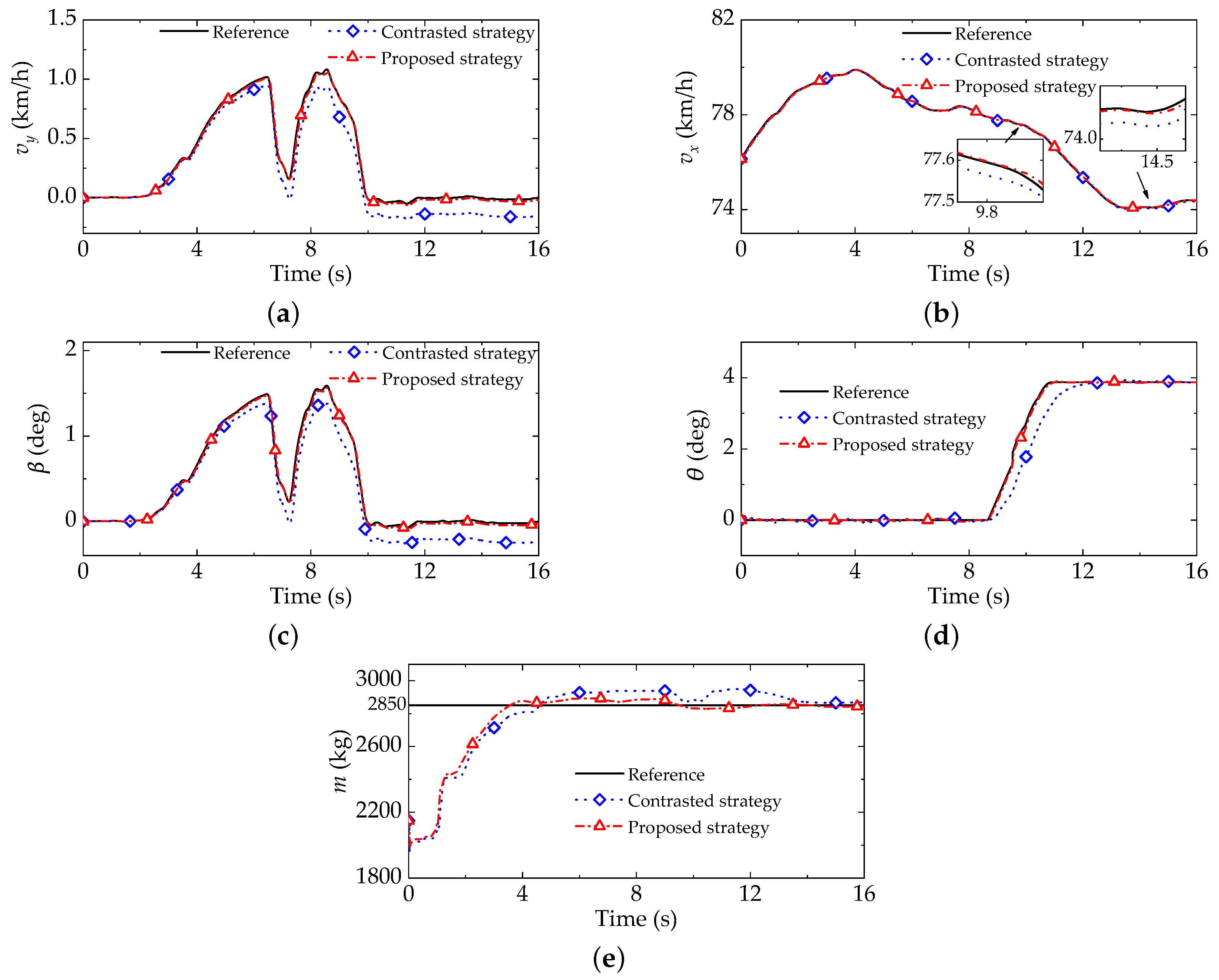
7.2. Driving Simulator Experiment
The driving simulator used in this experiment is provided by FORUM8, as
Figure 12. The driver is a 27-year-old male with three years of driving experience. The initial vehicle speed is 76 km/h, the vehicle mass is 2850 kg and the input signal of steering wheel is shown in
Figure 13.
The results of vehicle states in
Figure 14a–c show that the proposed strategy can follow the reference better in the most process, while there is a large deviation in the contrasted strategy. In the interval (9 s, 11 s) in
Figure 14d, the time delay of the proposed strategy is significantly smaller than the other. As for the vehicle mass in
Figure 14e, the proposed strategy reveals smaller errors as well.
The MAE and RMSE indicators of the driving simulator experiment are presented in
Figure 15. It is easy to see that the indicators of the proposed strategy are lower than the contrasted one. This proves that the proposed strategy’s performance is improved in statistical sense.
In general, the above-mentioned results demonstrate the effectiveness of the proposed joint soft-sensing strategy under diverse vehicle driving scenarios. Three modules in the strategy respectively implement the functions of estimating the vehicle state robustly, reducing the time delay of road slope observation and tracking the mutated vehicle mass. What is more, the information interaction within the strategy also provides virtual support for high-performance acquisition of multi-information.
8. Conclusions
This paper presents a joint soft-sensing strategy that can provide multi-information for automotive control under diverse vehicle driving scenarios. According to the distributed structure, the joint strategy realizes an information interaction among three modules. Based on the vehicle dynamic considering the road slope, the VBACKF is employed to adaptively estimate the vehicle states. To reduce the time delay, the road slope observer is implemented utilizing the slope prediction model and a fast response nonlinear cubic observer. The accuracy of vehicle mass is guaranteed by the information interaction and threshold judgment. Experimental results under diverse vehicle driving scenarios indicate the effectiveness of the proposed strategy and its performance superiority of low time delay, high accuracy and good stability.
For the development of the automated vehicle technology, this study may provide a new line of thinking for information soft-sensing and provide a necessary information guarantee for vehicle decision-planning and control.
Noticing that the omission of some potential factors may lead to unobserved heterogeneity, further research will be done on the accurate vehicle dynamics model, the position change of the COG, road adhesion coefficient, and so on. The real vehicle experiments will be carried out to make up for the unknown shortcoming in data.


