Performance Analysis and Design Considerations of the Shallow Underwater Optical Wireless Communication System with Solar Noises Utilizing a Photon Tracing-Based Simulation Platform

Abstract

The performance of the underwater optical wireless communication (UOWC) system is highly affected by seawater´s inherent optical properties and the solar radiation from sunlight, especially for a shallow environment. The multipath effect and degradations in signal-to-noise ratio (SNR) due to absorption, scattering, and ambient noises can significantly limit the viable communication range, which poses key challenges to its large-scale commercial applications. To this end, this paper proposes a unified model for underwater channel characterization and system performance analysis in the presence of solar noises utilizing a photon tracing algorithm. Besides, we developed a generic simulation platform with configurable parameters and self-defined scenarios via MATLAB. Based on this platform, a comprehensive investigation of underwater channel impairments was conducted including temporal and spatial dispersion, illumination distribution pattern, and statistical attenuation with various oceanic types. The impact of ambient noise at different operation depths on the bit error rate (BER) performance of the shallow UOWC system was evaluated under typical specifications. Simulation results revealed that the multipath dispersion is tied closely to the multiple scattering phenomenon. The delay spread and ambient noise effect can be mitigated by considering a narrow field of view (FOV) and it also enables the system to exhibit optimal performance on combining with a wide aperture.

1. Introduction

Underwater optical wireless communication (UOWC) has attracted considerable interest from both academia and industry as an effective solution to satisfy the rapidly increasing demands of underwater high-data-rate transmission. Compared with the conventional widely-used acoustic communication counterparts, UOWC systems have higher bandwidth, lower latency, and better security. These tremendous inherent merits enable it to be a promising alternative or complementary for various underwater applications such as imaging, real-time video transmission, and high-throughput sensor networks for natural oceanic resource exploration [1,2,3]. Besides, the future 6G coverage is anticipated to be expanded to remote areas, water surface, underwater, and satellite scenarios, which form an air-space-ground-sea integrated communication network. Thus, it is also regarded as one of the key potential technologies in the 6G underwater high-capacity wireless communication scenarios due to its large frequency spectrum bandwidth resources [4,5].

A hybrid acoustic/optical communication scheme is expected to play a significant role and take advantage of both technologies in the future underwater wireless sensor communication network (UWSN) and Internet of Underwater Things (IoUT). Figure 1 illustrates the basic architecture of a typical UWSN, which is composed of sensor nodes, solar-powered communication buoys, autonomous underwater vehicles (AUV), and underwater remotely operated vehicles (ROV). The optical base station (OBS) with seabed fixed or anchored sensors is capable of obtaining ocean monitoring data and communicating with ROVs, AUVs, or divers via optical/acoustic links. Then the ROVs or AUVs deliver the transmitted data to submarines, communication buoys, ships or other devices [6]. Above the sea level, the information exchange is accomplished through radio frequency (RF) or free space optical (FSO) communication links between ships and the onshore data stations. Despite all the aforementioned advantages, UOWC links suffer from severe channel impairments due to the seawater inherent optical properties (IOP), namely absorption and scattering effect. The absorption effect refers to an irreversible process in which water molecules and particles absorb photons and convert them into thermal or chemical potential energy. The scattering process alters photon propagation directions and causes time-varying multipath effects, i.e., spatial and temporal dispersion [7]. In addition, multiple scattering also leads to energy loss due to the reduction of arrived photons at the receiver plane, especially in poor water quality environment.

Many research efforts have been carried out for underwater channel characterization and performance analysis in order to cope with these issues. Previous related works have been mainly based on analytical, experimental measurement and numerical simulation approaches. Several researchers in [8,9,10] utilized the analytical method to solve the classical radiative transfer equation (RTE), which characterizes the light field passing through the scattering medium. However, this method involves a large number of assumptions and approximations to simplify the derivation process and results, and it is extremely difficult to derive accurate analytical solutions. Authors in [11,12] adopted Beer-Lambert’s law to model the line-of-sight (LOS) underwater optical wireless channels due to its simplicity. However, this way can only express spatial path attenuation rather than temporal dispersion. In terms of experimental channel measurement, researchers in [13] established an experimental testbed to study the LD-UOWC channel characteristics by measuring the intensity of the light transmitted through different types of water. To overcome these limitations, the Monte Carlo numerical simulation method was developed to solve RTE and model the underwater channel; several works were reported in [14,15,16,17,18,19]. In [14], a Monte Carlo (MC) based approach was proposed to investigate the light attenuation and time-domain broadening effects in different types of seawater channels, the impact of the water quality, communication distance, and receiver aperture were also analyzed. In [15,16], authors used the MC method and single-parameter chlorophyll concentration model to study the LED-UOWC scattering channel, the IOP, and path loss in different waters and different ranges were evaluated under various conditions. Authors in [17] adopted a double gamma function to fit the numerical simulation results of channel impulse response and investigated the fitting performance in coastal and harbor water. Using the Monte Carlo statistical method, authors in [18] simulated and analyzed the laser spot-expansion and time-domain broadening characteristics of the UOWC link. The most recent work was presented in [19], here they proposed a novel UOWC channel modeling method based on the mixture of two Gamma functions, the results were validated through Monte-Carlo simulations and exhibited reasonable agreement. The aforementioned works on UOWC channel modeling are summarized in

Table 1. Summary of UOWC (underwater optical wireless communication) channel modeling approaches of previous works.

Modeling Approach	Advantages	Shortcomings	Main Characteristics	Solar Irradiance	References
Beer–Lambert’s law	Simple and efficient	Inaccurate, unable to analyze the delay spread effect	Path loss (PL)	N	[11,12]
Experimental modeling	Real measured validation data	High cost, difficult to deduce the impact of transceiver configurations	PL, h(t)	N	[13]
Analytical RTE	Analytical results	Very difficult derivation	PL	N	[8,9,10]
Numerical RTE	Easy Programming	Low efficiency in case of error	PL, h(t), $t_{DS}$	N	[14,18]
Chlorophyl Monte-Carlo	Accurate in simulation environment	Less efficient for errors	PL, h(t), H(f),	N	[15,16]
MC-Curve Fitting	Accurate results	Time consuming	H(0), h(t), $t_{DS}$	N	[17,19]

. However, most works have selected to neglect solar radiation or just give a fixed value in shallow waters. There is also a lack of an efficient and intuitional model to take this effect into account. Besides, no existing works have presented a scalable simulation platform specially designed for UOWC, combining channel modeling and estimation. The design considerations of a practical shallow UOWC transceiver face several trade-offs between system specifications. While a larger aperture and wide FOV can capture more optical signals, they also bring more ambient light noises and thus it is hard to determine the optimal combinations.

To overcome such limitations, we established a scalable photon tracing-based simulation platform to characterize the underwater optical channel and investigate the UOWC system performance with strong solar irradiance. A more efficient and intuitional method is proposed to quantify the amount of solar noise level at the certain depths and its impact on the system performance is evaluated. The detailed algorithm procedure and framework of this platform are presented, which is convenient for users to define the transceiver specifications and environmental conditions without required previous experiences in the UOWC channel model or MATLAB programming. Utilizing this platform, we give a detailed study of the channel features in terms of time and spatial dispersion, and path loss. The temporal expansion and spatial attenuation with different system configurations (FOV, aperture) and oceanic types are quantified based on the channel impulse response and the statistical results derived from photon tracing simulation. The light illumination distribution pattern over the receiver plane is displayed to study the tracking and alignment difficulty for different optical sources (LED or LD). Different noise sources are analyzed and the ambient noise intensity is estimated based on the sea level downwelling solar irradiance. Eventually, the corresponding BER performance is presented to explore the effect of various FOV and apertures at different operation depths.

2. Principle

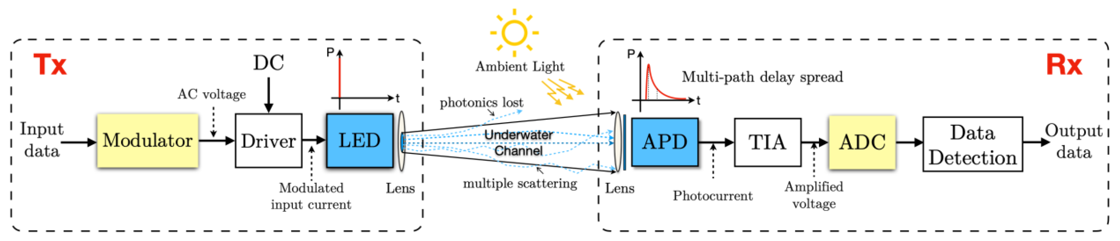
2.1. UOWC System Model

The schematic diagram of the typical UOWC system model is presented in Figure 2. At the transmitter side (Tx), the input binary bits are first modulated to drive the optical source via a driver circuit for emitting visible light signals. At the receiver side (Rx), after passing through the underwater channel, the optical signal is captured by a photodetector (PD), converted to photocurrent and amplified by a trans-impedance amplifier (TIA) to voltage values. Finally, the data is retrieved after analog-digital conversion (ADC) and the data detection process.

Obviously, the system performance is highly affected by two aspects, (i) spatial and temporal dispersion caused by the underwater medium multipath scattering phenomenon, (ii) electrical noises resulting from sunlight and hardware components such as PD and TIA (Figure 2). Moreover, in the shallow underwater environment, the water quality tends to be more turbid and ambient light is much stronger, which can exacerbate these problems. Typical attenuation coefficients for different oceanic types are summarized in

Table 2. Typical attenuation coefficients for different water types.

Water Type	a (m−1)	b (m−1)	c (m−1)
Pure sea	0.0405	0.0025	0.043
Clear ocean	0.114	0.037	0.151
Coastal	0.179	0.219	0.398
Turbid harbor	0.366	1.824	2.190

. The attenuation coefficient c describes the amount of energy loss of light propagating through the water medium and is defined as the sum of absorption a and scattering coefficients b. These coefficients are associated with the concentration of dissolved particles, planktonic matter, detritus, and change with different water types. The characteristics of the four major water types are as follows:

• Pure sea water—absorption effect is the major limiting factor. The light propagation trajectory is nearly a straight line due to the low scattering coefficient.
• Clear ocean water—Concentration of dissolved particles is higher than that in pure sea water, leading to an emerging scattering effect.
• Coastal water—Concentration of suspended matter and detritus becomes much higher in that it affects both absorption and scattering.
• Turbid harbor water—Concentration of planktonic matter, dissolved particles and mineral components is highest among the four water types, which can cause severe light scattering effect and attenuation.

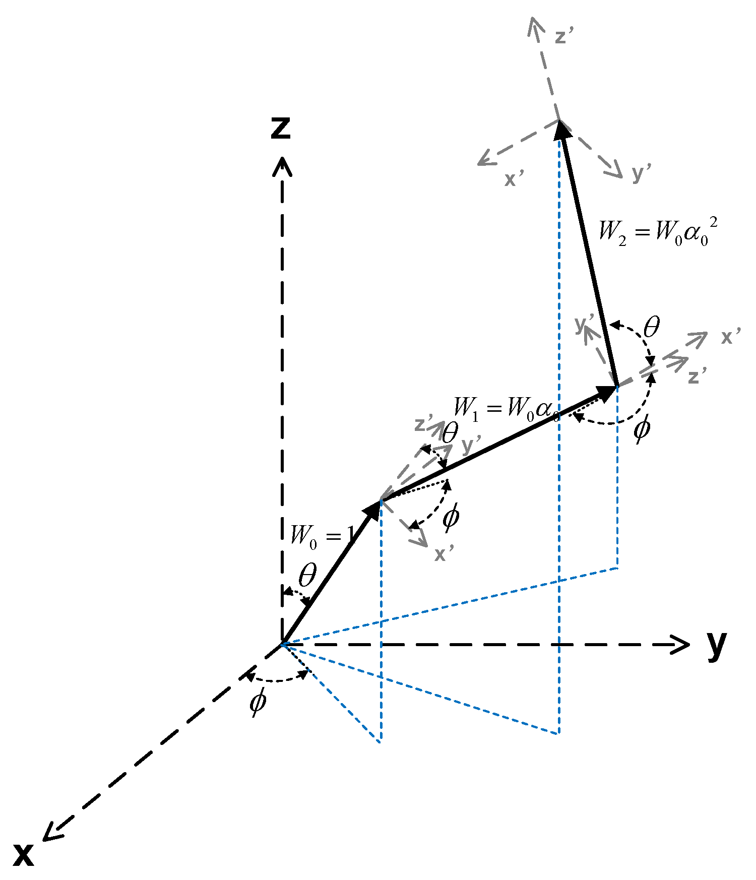
2.2. Photon Tracing Algorithm

We utilize a statistical Monte Carlo photon tracing algorithm (PTA) for underwater optical channel characterization and further performance analysis. The principle of this approach is to assume the light source as a collection of photons and obtain the final statistical results by tracking each propagation path from Tx to Rx through the seawater medium [20,21].

First, a large number of photons are randomly generated at the optical source, each with assigned attributes including initial location, transmitting direction, time and weight. The initial location can be deemed as (x, y, z) = (0, 0, 0) in Cartesian coordinates, the weight of each photon is set to unity with $W_0=1$, and the propagation starting time is $t=0$. The emitting direction is described by polar angle $\theta$ and azimuth angle $\varphi$. Considering the fact that the intensity of most optical sources is azimuthally symmetric,$\varphi$ is assumed to be uniformly distributed in the interval [0, 2π]. The polar angle is determined based on the spatial intensity distribution pattern of the light source. For LED-based diffuse links, the radiant intensity distribution is modeled as a generalized Lambertian profile [22], and expressed as:

$$R\left(\theta \right)=\frac{m+1}{2\pi }co{s}^m\left(\theta \right)$$

(1)

where m indicates the order of Lambertian emission and is related to the semi-angle at half-power, ${\theta }_{1/2}$, as $m_1=-In2/In\left(cos{\theta }_{1/2}\right)$. Then by normalizing radiation pattern $R\left(\theta \right)$ with $2\pi {{\displaystyle \int }}_0^{\pi /2}R\left(\theta \right)\sin \left(\theta \right)d\theta =1$ and equating $2\pi {{\displaystyle \int }}_0^{{\theta }_0^{LED}}R\left(\theta \right)\sin \left(\theta \right)d\theta ={ℝ}_1$. The polar and azimuth angle can be given as follows:

$$\{\begin{array}{c}{\theta }_0^{LED}=\arccos \left(\sqrt[m+1]{{ℝ}_1}\right)\\ {\varphi }_0^{LED}=2\pi {ℝ}_2\end{array}$$

(2)

in which ${ℝ}_1$ and ${ℝ}_2$ are random variables (RV) uniformly distributed in [0, 1]. Likewise, laser-based collimated link can be considered as a Gaussian beam profile and its starting directions of photons can be given by:

$$\{\begin{array}{c}{\theta }_0^{LD}={\theta }_{div/2}\times \sqrt{-ln\left({ℝ}_3\right)}\\ {\varphi }_0^{LD}=2\pi {ℝ}_4\end{array}$$

(3)

where ${\theta }_{div/2}$denotes the laser half divergence angle and is related to the beam waist, ${ℝ}_3$and ${ℝ}_4$ are also uniformly distributed RVs in the interval [0, 1]. Thus, the major difference between the LED and laser based UOWC channels is the initial emitting directions, the LED link is more diffusive whereas the laser beam is collimated. Afterwards, the starting orientations of photons can be described as cosine directions $(c_x,c_y,c_z)=\left(sin{\theta }_{0}cos{\varphi }_0, sin{\theta }_{0}sin{\varphi }_0,cos{\varphi }_0\right).$

While traveling through the underwater medium, the photons will interact with the particulate matter and water molecules, resulting in deviation from the original path and weight reduction (Figure 3). The propagation distance between two interaction events is defined as step size $\Delta s$ with its probability distribution function (PDF) based on the Beer Law: $p\left(\Delta s\right)=c\left(\lambda \right)e^{-c\left(\lambda \right)\Delta s}$, then $\Delta s$ can be simplified and randomly chosen as $\Delta s=-In{ℝ}_5/c\left(\lambda \right)$, in which ${ℝ}_5$ represents another RV, $c\left(\lambda \right)$ is the water attenuation coefficient. As shown in Figure 3, the weight of photon after each interaction is used to update as$W_{n+1}=W_n{\alpha }_0^{n+1}$, where ${\alpha }_0=b\left(\lambda \right)/c\left(\lambda \right)$ [23]. The new direction is described by the scattering polar angle ${\theta }_s$, which can be derived using the Henyey Greenstein scattering phase functions (HG-SPF), $\xi \left({\theta }_s,{\varphi }_s\right)$ [24]. Similarly as mentioned above, by equating $2\pi {{\displaystyle \int }}_0^{{\theta }_s}\xi \left({\theta }_s,{\varphi }_s\right)\sin \left(\theta \right)d\theta$ to an RV, the new direction is determined as:

$$\{\begin{array}{c}{\theta }_s=\arccos \left(1+s^2-{\left[\frac{1-s^2}{1-s+2s{ℝ}_6}\right]}^2/2s\right)\\ {\varphi }_s=2\pi {ℝ}_7\end{array}$$

(4)

where $s$ represents the asymmetric parameter related to the water quality, ${ℝ}_6$and ${ℝ}_7$ are two RVs in [0, 1]. Then the new photon coordinates are continuously updated and the tracking of a photon is terminated when its weight drops below a given threshold ($E_{th}={10}^{-6}$) or it reaches the receiver plane. That is to say, the photon falls within the receiver aperture and its polar angle is less than half of the field of view (FOV). After repeating the aforementioned tracing process, the corresponding attributes of captured photons are recorded for channel impulse response (CIR) plot and further analysis.

2.3. Noise Modeling

The UOWC system noises can be categorized into two parts, electrical noise and solar noise arising from the Rx components and ambient sunlight respectively. The electrical noise sources mainly consist of photocurrent shot noise, dark current noise, and thermal noise [25,26].

The shot noise is caused by random incident photons and the generated current flowing through the device, which is generally modeled as a Poisson distribution random process. Nevertheless, when the received optical signal power maintains a high level, that is to say, there is a significant increase in the incident photons, the Poisson distribution-based shot noise can be approximated to a Gaussian distribution model. Thus, its variance is expressed as:

$${\sigma }_{sn}^2=2eBMF\left(M\right)\left(I_{os}+I_{sr}\right)$$

(5)

where $e$ denotes the electron charge, $B$ is the bandwidth, $M$ represents the multiplication factor, $F\left(M\right)$ is the excess noise figure related to $M$ and the excess noise index, $I_{os}$ and $I_{sr}$ indicate the photocurrent generated at Rx from the optical signal and solar radiation, respectively. Similarly, the dark noise variance is given by:

$$\{\begin{array}{c}{\sigma }_{dn}^2=2eB{M}^{2}F\left(M\right)I_{db}+2eB{I}_{ds}\\ I_{dark}=I_{ds}+M{I}_{db}\end{array}$$

(6)

where $I_{dark}$ is the total dark current, $I_{db}$ and $I_{ds}$ represent the dark bulk and surface leakage currents, respectively. For a PIN-Rx, the multiplication factor $M_{PIN}$ and noise figure are always equal to one. In terms of an APD-Rx, these two factors are dependent on the reverse voltage, we commonly have $10<M_{APD}<200$, $F{\left(M\right)}_{APD}=\vartheta M_{APD}\left(1-\vartheta \right)\left(2-1/M_{APD}\right)$, in which $\vartheta$ is the holes/electrons ionization rate. The thermal noise mainly arises from the trans-impedance $R_L$ and can be classically modeled as a zero-mean Gaussian random process given by:

$${\sigma }_{tn}^2=4KTB/R_L$$

(7)

in which $K$ and $T$ denote the Boltzmann constant and the temperature in Kelvin, separately.

To evaluate the ambient light noise impact, we should first quantify the solar radiation level at a certain depth below the sea surface. In ocean optics, the ambient light becomes cumulatively diffusive and attenuates approximately exponentially with the depth after permeating into the seawater [27]. The downwelling plane irradiance is assumed as follows using the K function:

$$E_d\left(z,\lambda \right)=E_d\left(0,\lambda \right)exp\left[-{{\displaystyle \int }}_0^z{K}_d\left(z^{\prime },\lambda \right)d{z}^{\prime }\right]$$

(8)

where $E_d\left(0,\lambda \right)$ denotes the sea surface direct irradiance in $W\cdot m^{-2}\cdot n{m}^{-1}$, $K_d\left(z,\lambda \right)$ is the diffuse attenuation coefficient in $m^{-1}$, $\lambda$ is the wavelength in $nm$. Although $K_d\left(z,\lambda \right)$ is always related to depth and the wavelength, it is pretty complicated to derive the precise value at each level of depth and the accurate theoretical modeling of $K_d\left(z,\lambda \right)$ is out of the scope of this work. In addition,$K_d\left(z,\lambda \right)$ is independent of depth under several typical conditions such as in homogeneous water or far enough above the bottom in optically shallow water where the incident lighting mainly comes from the sun and sky [28]. Thus, for the convenience of estimation, the $K_d\left(z,\lambda \right)$ is assumed to be a constant at a certain depth range and Equation (8) can be simplified as $E_d\left(z,\lambda \right)=E_d\left(0,\lambda \right)exp\left[-K_d\left(\lambda \right)z\right]$. The experimental measurement of $K_d\left(\lambda \right)$ and $E_d\left(0,\lambda \right)$ has been conducted in several works [28,29,30]. The exact value of $E_d\left(0,\lambda \right)$ exhibits a huge difference under different climate conditions (i.e., clear or hazy) and the sun locations (i.e., zenith and azimuth angle). To present a worst-case analysis, we consider the clear weather and sun at its zenith based on the measured data in [24,28]. Then the photocurrent $I_{sr}$ generated at the Rx plane can be qualified as:

$$I_{sr}={\eta }_{QE}e{{\displaystyle \int }}_{450}^{530}{E}_d\left(0,\lambda \right)D_{f}exp\left[-K_d\left(\lambda \right)z\right]A_r\left[1-\cos \left(\phi \right)\right]{\eta }_{BF}\left(\lambda \right)d\lambda /\upsilon h$$

(9)

where ${\eta }_{QE}$ and ${\eta }_{BF}\left(\lambda \right)$ denote the quantum efficiency and band-pass filter transmittance, respectively. $A_r$ is the active detection area, $h$ is Planck’s constant,$D_f$ represents the direction dependence factor, $\upsilon$ is the optical frequency. Then the SNR at Rx can be given as:

$$\gamma ={\left({\eta }_{QE}eM{P}_T{{\displaystyle \int }}_0^{\infty }{h}_{PTA}\left(t,d\right)dt/\upsilon h\right)}^2/{\sigma }_n^2$$

(10)

in which ${\sigma }_n^2={\sigma }_{sn}^2+{\sigma }_{dn}^2+{\sigma }_{tn}^2$ represents the total noise variances.

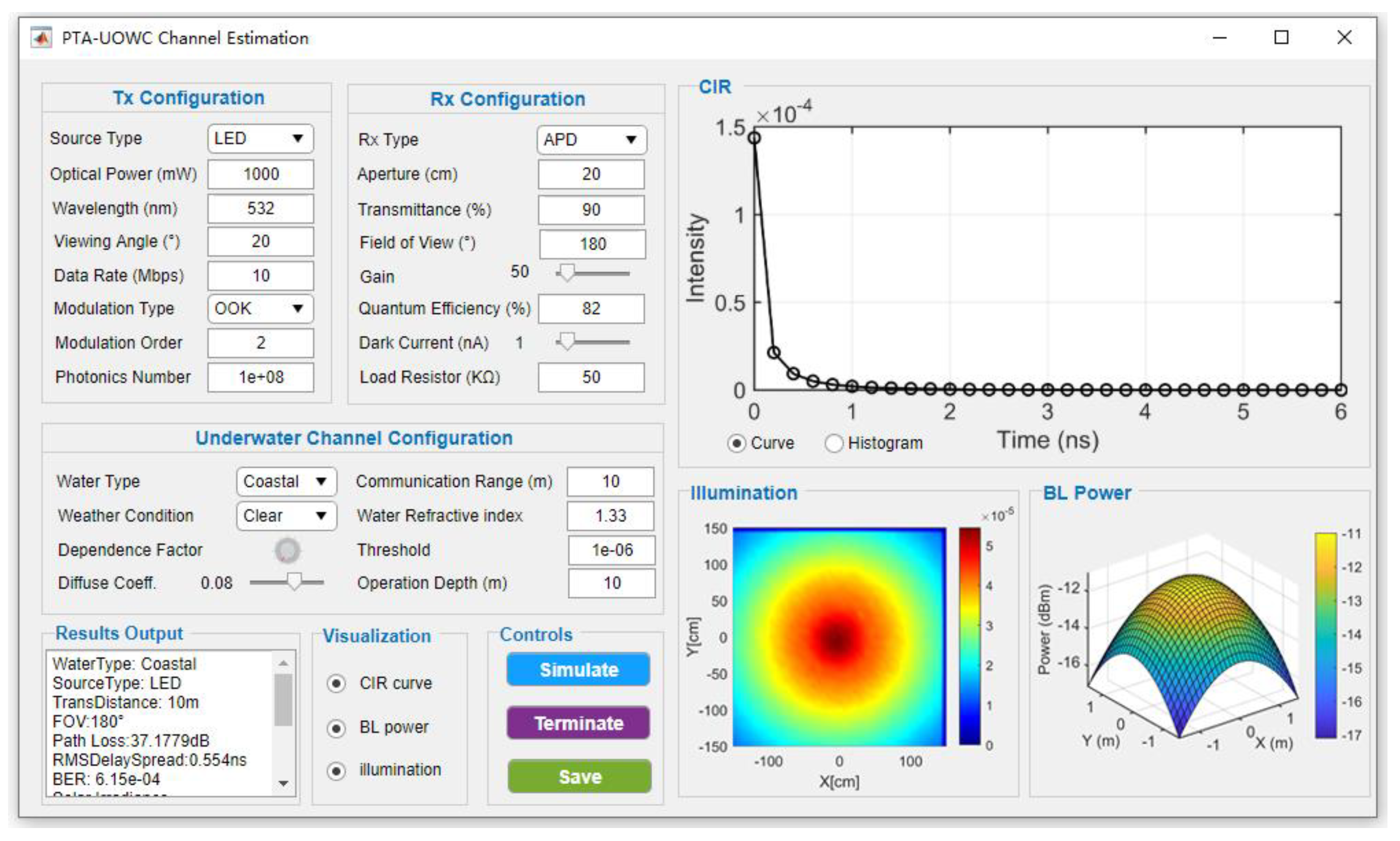
2.4. Graphical User Interface Design

In order to facilitate system design and numerical analysis, we developed a simulation platform of PTA-UOWC channel estimation with configurable parameters using MATLAB. The graphical user interface (GUI) of this app is presented in Figure 4, which is mainly composed of channel modeling, numerical results illustration, and performance indicators output. The upper left part of this GUI is divided into 3 major panels where users can freely set proper transceiver parameters and environment cases. It is to be noted that we use some slider components to guarantee the reasonable range of some input parameters such as gain, quantum efficiency, and dark current. Besides, in the zone of underwater channel configuration, several weather condition options are provided to differentiate the sea surface solar irradiance level based on the data reproduced from experimental results. After parameter initialization, users should select the visualization option and click the “Simulate” button to obtain the channel estimation results plotted in the right part of the GUI. Additionally, the channel estimation results and system performance indicators are displayed in the status panel including RMS delay spread, PTA and BL path loss and BER. The simulation figures and statistical results can be saved by clicking the “Save” button.

The Beer–Lambert law overestimates the link attenuation due to the implicit assumption that all the scattered photons are considered to be lost, while a quite large number of scattered photons are still very likely to get back to the Rx. However, it is only inaccurate in waters with high scattering coefficients such as coastal and turbid harbor waters. In pure sea and clear ocean water, the scattering effect is not obvious and the light travels almost in a straight line, thus the attenuation results derived from the BL law and the PTA simulation are very close. Besides, considering its simplicity and efficiency, it can be used to do rapid qualitative analysis to see the impact of changing one system parameter on the system performance. Although the value is not accurate, we can observe the trend [31]. Thus, our simulation platform also provides such a function for fast evaluation. Overall, this simulation platform offers a concise and efficient approach for users to obtain an intuitive understanding of the UOWC link performance. It is much more convenient to construct input specifications, define different scenarios, and process the output data. Besides, users are not required to have expertise in UOWC models or programming skills and need not worry about an illogical input since we have controlled several variables within reasonable bounds. This user-friendly GUI incorporates the underwater channel characterization with the solar irradiance model and different modulation schemes, which enable the designer to make preliminary judgments and choose appropriate hardware components

3. Results and Discussions

In this section, we present the numerical simulation results for various scenarios based on the established simulation platform. It is worth mentioning that the characteristics of the optical channel in seawater are affected by many factors, mainly the seawater environment and the transceiver configurations and thus there exist many combination cases. To be more representative and not too complicated, we provide the simulation results under some typical configurations and our analysis focuses on spatial attenuation and temporal dispersion together with system BER performance with solar noises. Besides, although we mainly studied the LED-based diffusive cases, some laser-based results are also presented for comparison and improved analysis. Several important parameters for simulation are summarized in

Table 3. UOWC system configuration.

Parameter	Symbol	Value
LED semi-angle at half power	${\theta }_{1/2}$	(15°, 20°)
Laser divergence angle	${\theta }_{div/2}$	(0.75, 1) mrad
Link range	$d$	1–35 m
Water refractive index	$n$	1.33
Total number of transmitted photons	$N_T$	108
Aperture diameter	$A_d$	5, 11, 20 cm
Depth	$D$	10, 25, 100 m
Weight threshold	$E_{th}$	10−6

.

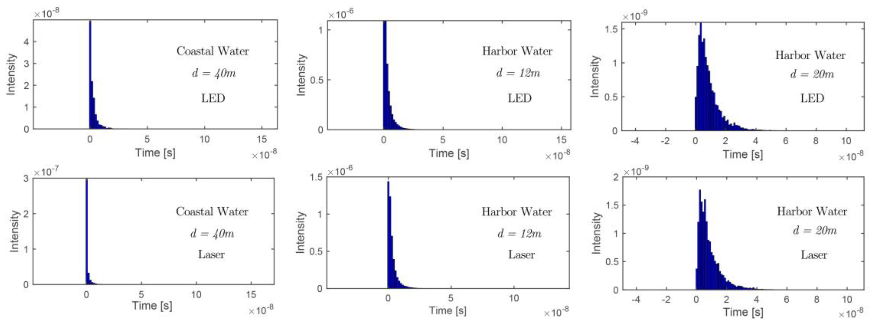
3.1. Temporal Dispersion

To evaluate the time dispersive properties of the UOWC channel, we should first derive the CIR after performing the PTA simulation. Since the statistical results such as the weight and corresponding arrival time of each detected photon have been recorded, we can calculate the summation of the weights within a specific time slot (i.e., 0.2 ns), normalize it by the total emitting photons weights and then plot the CIR curve. Thus, for the jth time slot, this process is described as [32]:

$${\rho }_j=\frac{1}{N_T{W}_0}{\displaystyle \sum }_i{W}_i{{\displaystyle \int }}_{\left(j-1\right)T_r}^{j{T}_r}\delta \left(t-T_i\right)dt$$

(11)

where $W_i$ is the weight of the ith detected photon corresponding to the arrival time $T_i$, $T_r$ is the time resolution, $N_T$ represents the total number of transmitted photons, and the latter integral is expressed as ${{\displaystyle \int }}_{\left(j-1\right)T_r}^{j{T}_r}\delta \left(t-T_i\right)dt=\{\begin{array}{c}1 for T_i\in \left[\left(j-1\right)T_r,j{T}_r\right]\\ 0 for T_i\notin \left[\left(j-1\right)T_r,j{T}_r\right]\end{array}$.

Afterwards, the temporal dispersion effect can be quantified by computing the root mean square (RMS) delay spread $t_{DS}$ given by:

$$\{\begin{array}{c}{t}_{DS}=\sqrt{{{\displaystyle \int }}_{-\infty }^{\infty }{\left(t-t_0\right)}^2{h}^2\left(t\right)dt/{{\displaystyle \int }}_{-\infty }^{\infty }{h}^2\left(t\right)dt}\\ t_0={{\displaystyle \int }}_{-\infty }^{\infty }t{h}^2\left(t\right)dt/{{\displaystyle \int }}_{-\infty }^{\infty }{h}^2\left(t\right)dt \end{array}$$

(12)

in which $t_0$ is the mean excess delay spread.

Figure 5 depicts the CIR for four different water types with different system configurations (i.e., FOV). The curve smoothness is associated with the given time resolution $T_r$ and the total number of simulated photons $N_T$. We consider the Rx with an aperture of 50 cm and Tx with a divergence angle of 15°. It can be clearly observed that the intensity drops significantly from the peak in 100 m pure sea water and there is almost no “trailing” phenomenon on the curve. The trajectory of photons is nearly a straight line to the Rx. As the water turbidity increases, the delay spread tends to be more severe with the fact that the 9 m link in harbor water exhibits a worse channel quality than the longer 29 m coastal link or even the 50 m clear ocean link. This is because a more turbid water medium with larger $c\left(\lambda \right)$ leads to a greater number of scattering events, where $\Delta s$ is smaller and $E_{n+1}$ drops below the threshold faster. Therefore, the time delay of arrival photons increases resulting in serious temporal dispersion. At the same time, it can be intuitively found that the delay spread tends to be larger with the increase of FOV. This result is also easy to explain considering the fact that Rx with wider FOV is more likely to capture those photons which have deviated from the optical axis after multiple scattering events. To be more persuasive, the RMS delay spread $t_{DS}$ is also calculated using (12) to characterize the channel dispersion. We obtain $t_{DS}$ = (0.74 ns, 1.16 ns, 2.73 ns) and (1.21 ns, 1.44 ns, 2.76 ns) corresponding to FOV = (15°, 35°, 180°) for coastal and harbor water, respectively. It is easy to see that the$t_{DS}$ rises with the increase of FOV and water turbidity, which verifies the aforementioned analysis. Additionally, since the channel dispersion can bring inter-symbol interference (ISI) and limit the system performance, we can also estimate the maximum transmitted data rate through the optical wireless channel without the requirement of equalization by using $R_b\le 1/10t_{DS}$.

Furthermore, our simulation platform provides another option for CIR plots to make the results more intuitive, namely histogram displays. In this way, the time difference between the first and last arrival photons is divided into 100 bins, then the histogram of intensity versus time (Figure 6) can be easily obtained by calculating the normalized weights within each bin similarly as elaborated before. Here we give the LD-based numerical results in order to make a comparison between the diffusive and collimated links in Figure 6. It can be found that the LD-based channel shows less channel dispersion effect than the LED-based link due to its collimation and much smaller divergent angle.

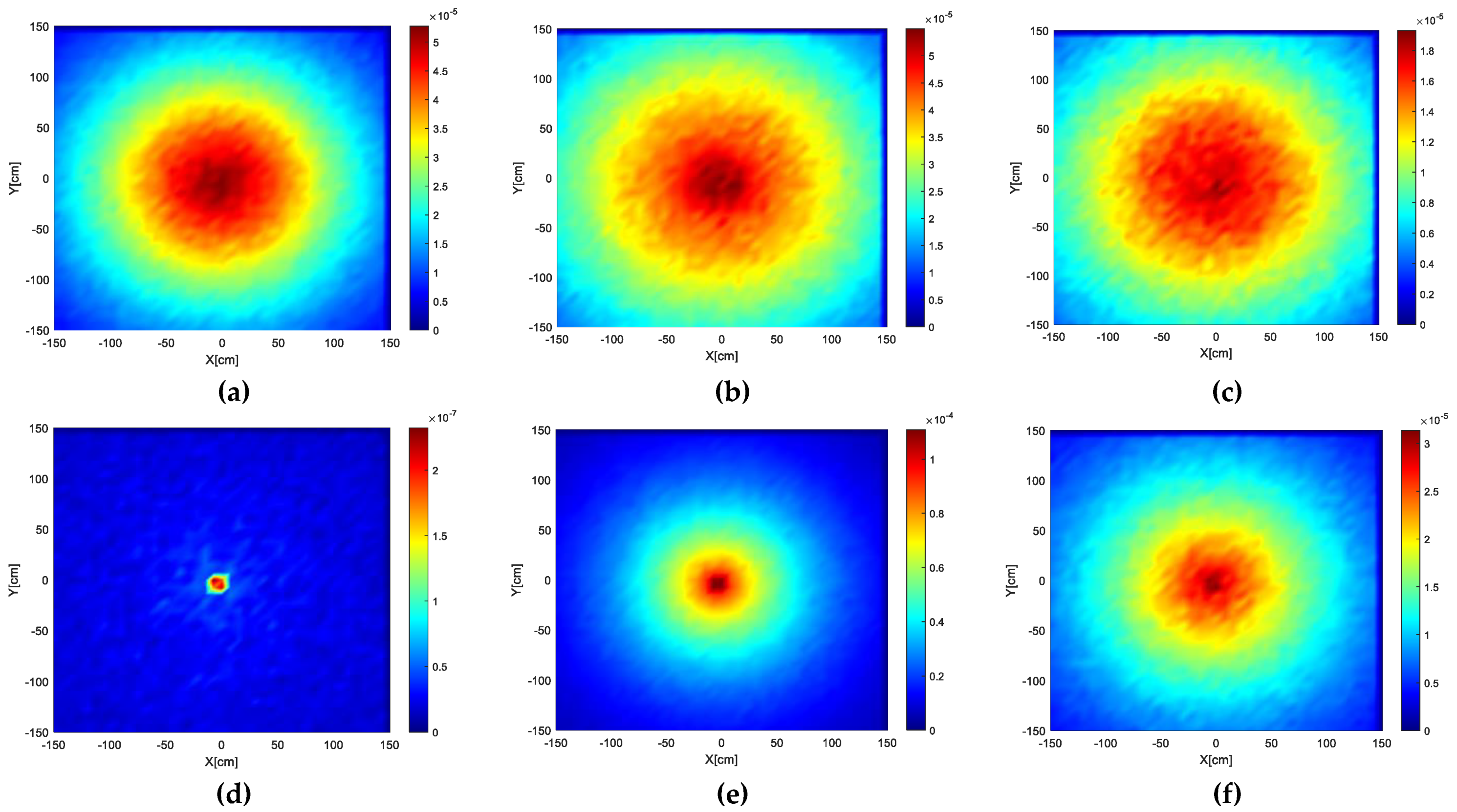
3.2. Spatial Illumination Pattern

In this section, we investigate the spatial distribution of illumination at a square receiver plane with an area of 3 × 3 m² to better describe the channel spatial dispersion characteristic. The whole area is divided into 50 × 50 pixels, with each occupying the area of 6 × 6 cm². Then we compute the normalized intensity of the strike photons within each pixel over a specific time slot after performing PTA. As Figure 7a–c shows, for LED-based links, the received intensity tends to spread uniformly from the center to its periphery and become weaker with the increase of water turbidity. For laser-based paths, the energy is concentrated on the center spot, and there is almost no such beam spread in coastal water (Figure 7d). However, in the case of turbid harbor water, the received light intensity always exhibits significant spatial spread whether LED or laser (Figure 7e,f). Although spatial dispersion phenomenon can aggravate the energy loss and time-domain broadening effect, a divergent link also reduces the tracking and alignment difficulties, making it feasible to cover more mobile users.

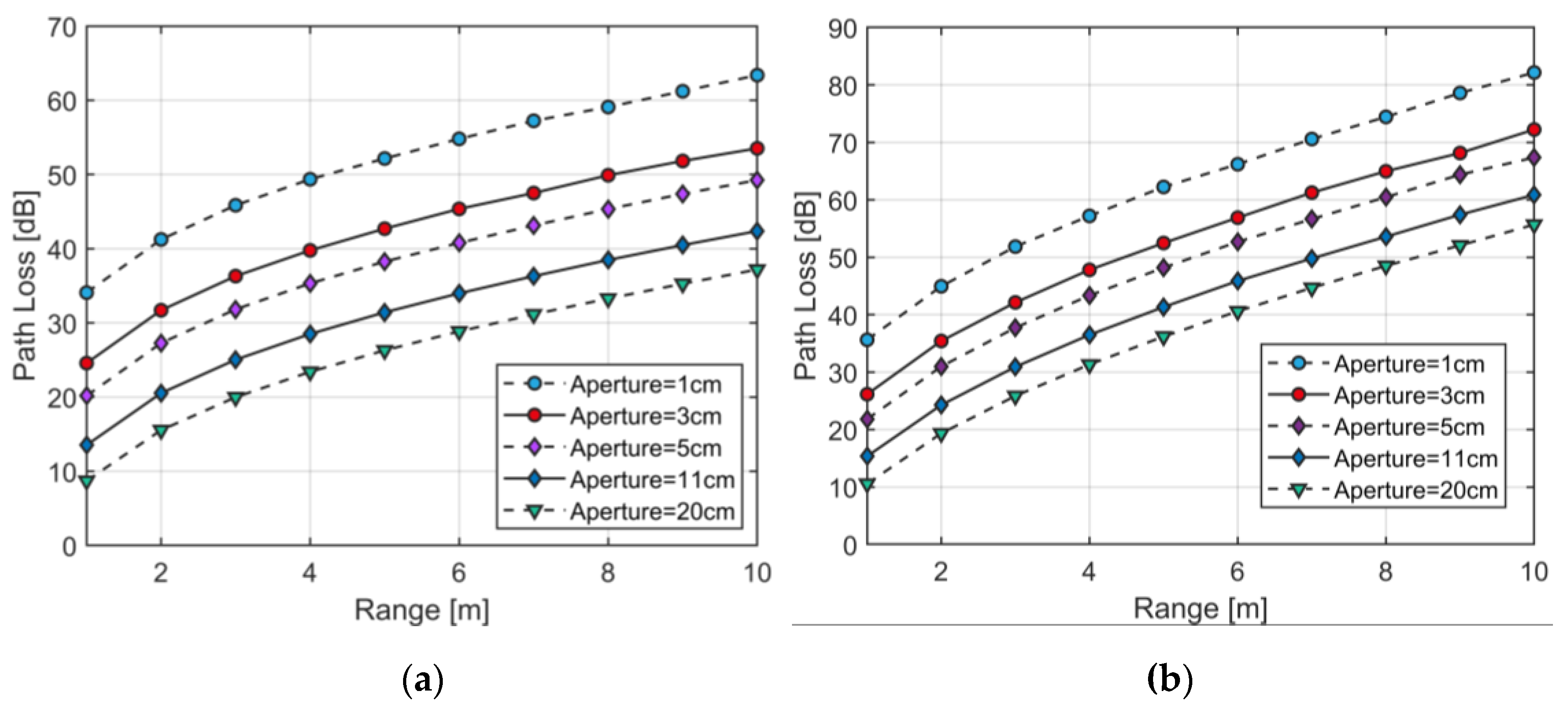
3.3. Statistical Attenuation

As we mentioned before, the Beer–Lambert law overestimates the link attenuation because it abandons all the scattered photons that have possibilities to return to the aperture, especially in the coastal and turbid harbor waters. Thus, we investigated the deviation of the BL path loss by exploiting the numerical simulation. After the simulation, the link attenuation is determined by $PL\left(dB\right)=\lg \left({\displaystyle \sum }_{i=1}^{N_r}{W}_i/N_T{W}_0\right)$, where $N_r$ represents the number of received photons. Figure 8 shows the comparison of the path loss obtained by BL computation (dashed line) and PTA simulation (solid line). We can verify that the BL results are much larger and there is a growing gap with the increase of water turbidity and distance. The more turbid water and longer communication range implies more interactions with particles and scattering times such that a bigger difference is observed.

Figure 9 depicts the BL-based three-dimensional spatial distribution of optical power on a 3 × 3 m² receiver plane after 10 m transmission under different water conditions. It may seem a little strange that the received power is so much lower in turbid harbor water than that in other water types, but the fact that its corresponding attenuation coefficient is 2.1 m⁻¹, whereas the value is 0.398 m⁻¹ in coastal ocean needs to be considered. Therefore, according to $PL\left(dB/m\right)=10\lg \left(e^{-c}\right)\approx -4.343c$, a big difference of path loss in a 10 m channel is reasonable and consistent with the data in Figure 10.

Figure 10 illustrates the statistical results of path loss versus communication distance derived from the proposed PTA numerical simulation with different Rx apertures in coastal and turbid harbor waters. The total attenuation consists of the geometry loss and seawater optical loss. As the aperture rises from 1 cm to 20 cm, a decrease of the link attenuation can be witnessed. This is because the larger Rx area means a greater probability to capture scattered photons in such poor quality water medium.

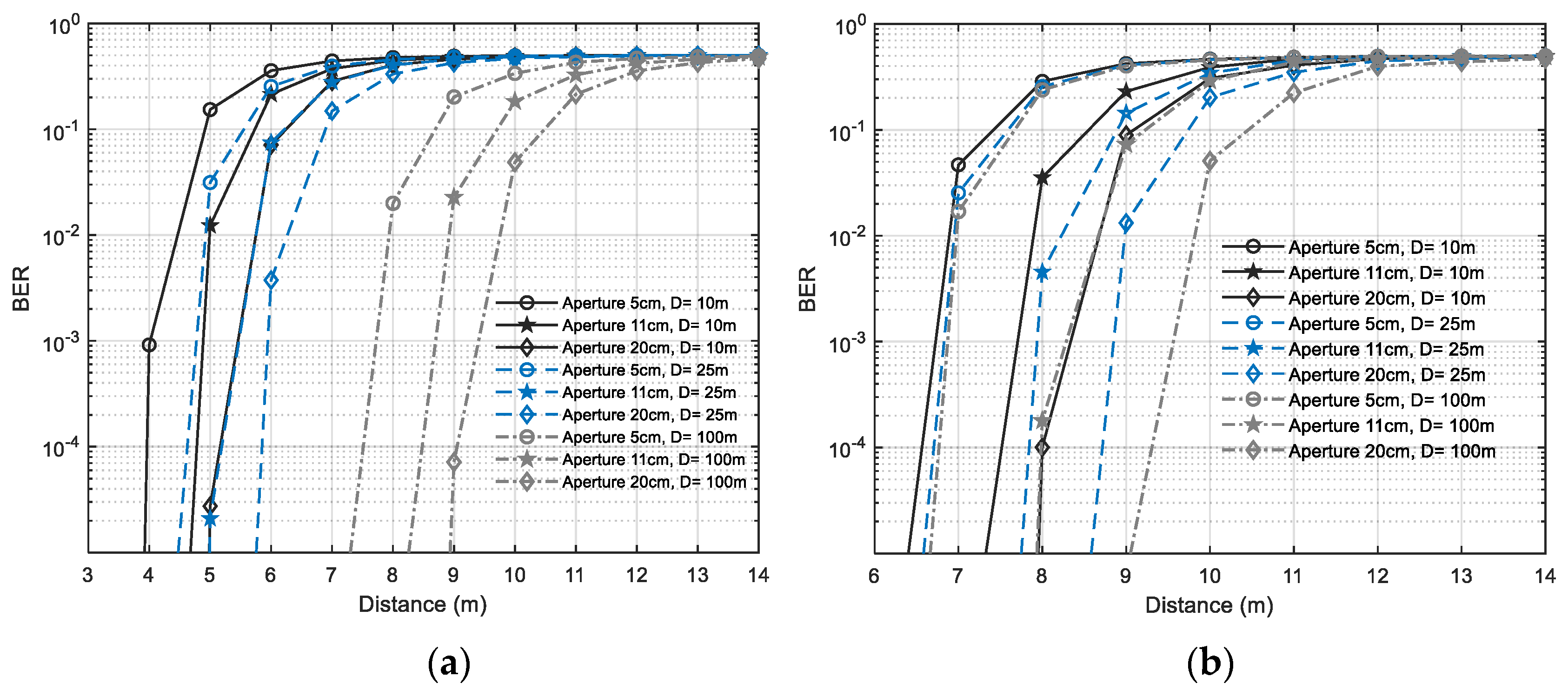
3.4. BER Performance

After obtaining the statistical channel path loss, we can evaluate the BER performance combined with the Rx configuration and solar radiation level. We considered the case of on-off keying modulation (OOK) due to its simplicity and widespread usage in the real-time UOWC system. The transceivers are assumed to be perfectly aligned. Figure 11 and Figure 12 show the BER performance versus communication range under various system specifications (FOV, aperture diameter). In order to quantify the ambient light noises impact, we place the transceiver at different depths. By using the proposed model mentioned before, the dowelling solar irradiance values at these operation depths are 0.0062, 0.0019, and 4.65 × 10⁻⁶ W/(m²·sr·nm), the lines of the same color represent cases at the same depths, with black, blue, and gray corresponding to 10 m, 25 m and 100 m, respectively.

It is apparent in Figure 11 and Figure 12 that increasing the aperture diameters from 5 cm to 20 cm can certainly improve the system performance at the same depth and this enhancement becomes a little more obvious in deeper water. The reason is, that while a larger aperture can detect more optical signals from Tx, it also receives stronger solar radiation in the shallow underwater environment. In the deep sea, however, the downwelling irradiance from sunlight becomes quite weak such that the raising of an aperture can deliver more performance improvement. It is worth mentioning that we assumed the attenuation coefficient remains the same at different depths for the worst-case analysis, whereas the water turbidity level drops with the increase of depths in reality. Thus, the reliable communication range in deep sea may be longer than the simulation results. Besides, the BER performance seems to be more sensitive to the depth with larger FOV using the same Rx aperture. If we consider the target BER of 10⁻⁴ and the aperture diameter of 11 cm, the viable communication range is extended from 8 m to 18 m with the water depth varying from 10 m to 100 m when FOV = 180°. Nevertheless, for the case of FOV = 15°, the distance increases from 19 m to 20.5 m. Likewise, considering that a narrow FOV has already restricted most of the sunlight in shallow water, it is reasonable that the increase of working depth has little impact on the performance improvement.

3.5. Design Considerations

Based on the above simulation results and analysis, we provide the overall design considerations for the UOWC system.

• Tx considerations: The optical source determines the optical output power and light divergence. The choice of LED or laser is scenario-specific and depends on the degree of alignment difficulty, if the tracking and pointing equipment is available for just point-to-point link, the collimation property and large power of laser (Figure 6) can help mitigate the temporal dispersion to achieve longer range and higher data rate. If the alignment is hard or more Rx users need to be covered, LED is a good choice. However, in turbid waters, illumination patterns of LED and laser both show significant spatial spread at the Rx plane (Figure 7), thus, the LED no longer has the merit of easy alignment and laser should be used under such a condition.
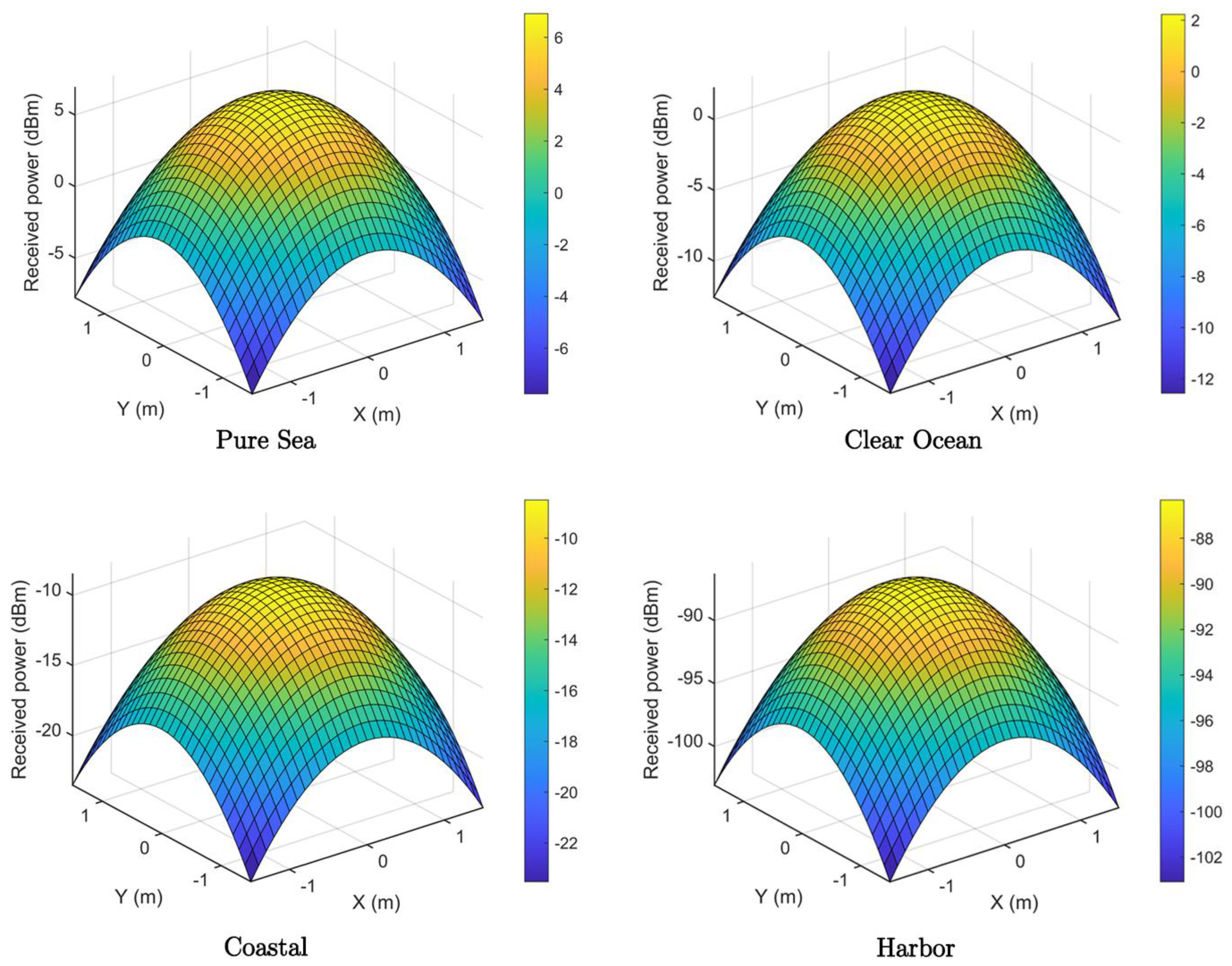
• Rx considerations: Although more optical signals can be received by using larger aperture size and wider FOV, they also result in more solar noises captured at the Rx in the shallow UOWC environment. Based on the simulation results of BER performance (Figure 11 and Figure 12), we suggest employing a large aperture combined with a narrow FOV angle to guarantee enough optical power at the Rx plane (Figure 10) and mitigate the SNR degradation. In addition, the optical filter in front of the detector is also important in determining the Rx’s sensitivity to solar irradiance radiation. An optical filter with narrow bandwidth can reduce the system FOV and suppress ambient noises.

4. Conclusions

In conclusion, a comprehensive simulation platform was established combining channel modeling with performance evaluation under solar irradiance based on the photon tracing algorithm. The user-friendly GUI facilitates both the system configuration and visualizing simulation results. We also analyzed the trade-off between different codependent factors such as FOV and apertures. Simulation results indicate that both diffusive and collimated links in harbor water exhibit serious spatial spread and the temporal dispersion becomes more severe with the increase of FOV, water turbidity, divergence angle, and link range, thus limiting the reliable maximum transmission data rate. Furthermore, a narrow FOV and wide aperture size can mitigate the SNR degradation resulting from ambient noises and statistical attenuation, and optimal BER performance is observed. This study offers valuable insights into the practical UOWC system design for different oceanic scenarios with strong ambient noises and is also beneficial for developers to select proper hardware devices and estimate reliable link performance. In further work, we will extend the capabilities of the simulation platform to take the turbulence effect into account.

References

1. Zeng, Z.; Fu, S.; Zhang, H.; Dong, Y.; Cheng, J. A survey of underwater optical wireless communications. IEEE Commun. Surv. Tutor. 2016, 19, 204–238. [Google Scholar] [CrossRef]
2. Khalighi, M.A.; Uysal, M. Survey on free space optical communication: A communication theory perspective. IEEE Commun. Surv. Tutor. 2014, 16, 2231–2258. [Google Scholar] [CrossRef]
3. Li, J.; Yang, B.; Ye, D.; Wang, L.; Fu, K.; Piao, J.; Wang, Y. A real-time, full-duplex system for underwater wireless optical communication: Hardware structure and optical link model. IEEE Access 2020, 8, 109372–109387. [Google Scholar] [CrossRef]
4. Yang, P.; Xiao, Y.; Xiao, M.; Li, S. 6G wireless communications: Vision and potential techniques. IEEE Netw. 2019, 33, 70–75. [Google Scholar] [CrossRef]
5. Lee, Y.U. Secure Visible Light Communication Technique Based on Asymmetric Data Encryption for 6G Communication Service. Electronics 2020, 9, 1847. [Google Scholar] [CrossRef]
6. Lian, J.; Gao, Y.; Wang, H. Underwater optical wireless sensor networks using resource allocation. Telecommun. Syst. 2019, 71, 529–539. [Google Scholar] [CrossRef]
7. Sun, X.; Kang, C.H.; Kong, M.; Alkhazragi, O.; Guo, Y.; Ouhssain, M.; Ooi, B.S. A review on practical considerations and solutions in underwater wireless optical communication. J. Lightwave Technol. 2020, 38, 421–431. [Google Scholar] [CrossRef] [Green Version]
8. Cochenour, B.M.; Mullen, L.J.; Laux, A.E. Characterization of the beam-spread function for underwater wireless optical communications links. IEEE J. Ocean. Eng. 2008, 33, 513–521. [Google Scholar] [CrossRef]
9. Jaruwatanadilok, S. Underwater wireless optical communication channel modeling and performance evaluation using vector radiative transfer theory. IEEE J. Sel. Areas Commun. 2008, 26, 1620–1627. [Google Scholar] [CrossRef]
10. Li, C.; Park, K.H.; Alouini, M.S. On the use of a direct radiative transfer equation solver for path loss calculation in underwater optical wireless channels. IEEE Wireless. Commun. Lett. 2015, 4, 561–564. [Google Scholar] [CrossRef] [Green Version]
11. Smart, J.H. Underwater Optical Communications Systems Part 1: Variability of Water Optical Parameters. In Proceedings of the IEEE Military Communications Conference (MILCOM’05), Atlantic City, NJ, USA, 17–20 October 2005; pp. 1140–1146. [Google Scholar]
12. Cochenour, B.; Mullen, L.; Muth, J. Temporal response of the underwater optical channel for high-bandwidth wireless laser communications. IEEE J. Ocean. Eng. 2013, 38, 730–742. [Google Scholar] [CrossRef]
13. Hanson, F.; Radic, S. High bandwidth underwater optical communication. Appl. Opt. 2008, 47, 277–283. [Google Scholar] [CrossRef] [PubMed]
14. Gabriel, C.; Khalighi, M.A.; Bourennane, S.; Léon, P.; Rigaud, V. Monte-Carlo-based channel characterization for underwater optical communication systems. J. Opt. Commun. Netw. 2013, 5, 1–12. [Google Scholar] [CrossRef] [Green Version]
15. Liu, W.; Zou, D.; Wang, P.; Xu, Z.; Yang, L. Wavelength Dependent Channel Characterization for Underwater Optical Wireless Communications. In Proceedings of the IEEE International Conference on Signal Processing, Communications and Computing (ICSPCC), Guilin, China, 5–8 August 2014; pp. 895–899. [Google Scholar]
16. Liu, W.; Zou, D.; Xu, Z.; Yu, J. Non-Line-of-Sight Scattering Channel Modeling for Underwater Optical Wireless Communication. In Proceedings of the IEEE International Conference on Cyber Technology in Automation, Control, and Intelligent Systems (CYBER), Shenyang, China, 8–12 June 2015; pp. 1265–1268. [Google Scholar]
17. Dong, F.; Xu, L.; Jiang, D.; Zhang, T. Monte-Carlo-based impulse response modeling for underwater wireless optical communication. Prog. Electromagn. Res. 2017, 54, 137–144. [Google Scholar] [CrossRef] [Green Version]
18. Yang, Y.; He, F.; Guo, Q.; Wang, M.; Zhang, J.; Duan, Z. Analysis of underwater wireless optical communication system performance. Appl. Opt. 2019, 58, 9808–9814. [Google Scholar] [CrossRef]
19. Boluda-Ruiz, R.; Rico-Pinazo, P.; Castillo-Vázquez, B.; García-Zambrana, A.; Qaraqe, K. Impulse Response Modeling of Underwater Optical Scattering Channels for Wireless Communication. IEEE Photon. J. 2020, 12, 1–14. [Google Scholar] [CrossRef]
20. Cox, W.; Muth, J. Simulating channel losses in an underwater optical communication system. J. Opt. Soc. Am. 2014, 31, 920–934. [Google Scholar] [CrossRef]
21. Leathers, R.A.; Downes, T.V.; Davis, C.O.; Mobley, C.D. Monte Carlo Radiative Transfer Simulations for Ocean Optics: A Practical Guide; Tech. Rep. NRL/MR/5660–04-8819; Naval Research Lab: Washington, DC, USA, 2004. [Google Scholar]
22. Ghassemlooy, Z.; Popoola, W.O.; Rajbhandari, S. Optical Wireless Communications System and Channel Modelling with MATLAB®, 2nd ed.; CRC Press: Boca Raton, FL, USA, 2012; pp. 81–90. [Google Scholar]
23. Khalil, R.A.; Babar, M.I.; Saeed, N.; Jan, T.; Cho, H.S. Effect of link misalignment in the Optical-Internet of underwater things. Electronics 2020, 9, 646. [Google Scholar] [CrossRef] [Green Version]
24. Mobley, C.D. Light and Water: Radiative Transfer in Natural Waters; Academic Press: Cambridge, MA, USA, 1994. [Google Scholar]
25. Zhou, H.; Zhang, M.; Wang, X.; Ren, X. Implementation of High Gain Optical Receiver with the Large Photosensitive Area in Visible Light Communication. In Proceedings of the Asia Communications and Photonics Conference (ACP), Chengdu, China, 2–5 November 2019; p. M4A.101. [Google Scholar]
26. Xu, F.; Khalighi, M.A.; Bourennane, S. Impact of Different Noise Sources on the Performance of PIN-and APD-based FSO Receivers. In Proceedings of the 11th International Conference on Telecommunications (ConTEL), Graz, Austria, 15–17 June 2011; pp. 211–218. [Google Scholar]
27. Duntley, S.Q. Light in the sea. J. Opt. Soc. Am. 1963, 53, 214–233. [Google Scholar] [CrossRef]
28. Mobley, C.D. Ocean Optics Web Book. Available online: https://www.oceanopticsbook.info/view/light-and-radiometry/introduction (accessed on 6 January 2021).
29. Lee, Z.P.; Darecki, M.; Carder, K.L.; Davis, C.O.; Stramski, D.; Rhea, W.J. Diffuse attenuation coefficient of downwelling irradiance: An evaluation of remote sensing methods. J. Geophys. Res. Ocean. 2005, 110, 1–9. [Google Scholar] [CrossRef]
30. Nababan, B.; Louhenapessy, V.S.; Arhatin, R.E. Downwelling Diffuse attenuation coefficients from in situ measurements of different water types. Int. J. Remote Sens. Earth Sci. 2013, 10, 122–132. [Google Scholar] [CrossRef] [Green Version]
31. Ju, M.; Huang, P.; Li, Y.; Shi, H. Effect of Receiver’s Tilted Angle on the Capacity for Underwater Wireless Optical Communication. Electronics 2020, 9, 2072. [Google Scholar] [CrossRef]
32. Zhang, M.; Zhang, Y.; Yuan, X.; Zhang, J. Mathematic models for a ray tracing method and its applications in wireless optical communications. Opt. Express 2010, 18, 18431–18437. [Google Scholar] [CrossRef] [PubMed]
Figure 1. Architecture of an underwater wireless communication sensor network.
Electronics 10 00632 g001
Figure 2. Schematic Diagram of the UOWC system model.
Electronics 10 00632 g002
Figure 3. Multiple scattering path of each photon.
Electronics 10 00632 g003
Figure 4. The graphical user interface of the PTA-UOWC simulation platform.
Electronics 10 00632 g004
Figure 5. Illustration of the CIR curve for different water types under various system configurations.
Electronics 10 00632 g005
Figure 6. Illustration of CIR histogram of diffusive and collimated links for coastal & harbor water.
Electronics 10 00632 g006
Figure 7. Spatial illumination distribution at the received square plane for LED-based diffusive link in (a) 10 m coastal water, (b) 5 m harbor water, (c) 6 m harbor water, and Laser-based collimated link in (d) 35 m coastal water, (e) 5 m harbor water, (f) 6 m harbor water.
Electronics 10 00632 g007
Figure 8. Path loss derived by the BL-analytical method and PTA simulation.
Electronics 10 00632 g008
Figure 9. Spatial distribution of optical power in the received plane.
Electronics 10 00632 g009
Figure 10. Path loss for different ranges with different apertures (a) coastal water, (b) turbid harbor water.
Electronics 10 00632 g010
Figure 11. BER performance versus communication distance with different apertures and operation depths in coastal water for (a) FOV = 180°, (b) FOV = 15°.
Electronics 10 00632 g011
Figure 12. BER performance versus communication distance with different apertures and operation depths in turbid harbor water for (a) FOV = 180°, (b) FOV = 15°.
Electronics 10 00632 g012