Comparisons of Modeling Methods for Fractional-Order Cuk Converter

Abstract

In this paper, several modeling methods for the continuous current mode (CCM) fractional-order Cuk converter are investigated. First, the state space averaging method is used to establish the model. Based on this model, the expressions of inductors’ current and capacitor voltage as well as the transfer functions are derived. Then, the equivalent small parameter method (ESPM) is employed to model the converter. Based on the Oustaloup filter principle, the approximate models of fractional-order capacitor and inductors are constructed, which consist of integer-order components, to build the circuit model (CM) of the converter. In addition, the numerical model (NM) of the converter is established. Simulation results are provided to compare the modeling methods, which show that the ESPM has some advantages over the other methods. Finally, the hardware-in-the-loop experiment is conducted to verify the effectiveness of the circuit model.

1. Introduction

The theory of fractional calculus has been proposed for more than 300 years. However, at the beginning, most scholars only carried out the theoretical research. It was not until 1960 that there was a major breakthrough in its physical meaning and practical foundation. Among them, the Italian scholars Caputo and Mainardi studied the energy consumption problem based on the fractional derivative; Slovak scholar Podlubny proposed a fractional proportional-integral-derivative controller and its design method; French scholar Oustaloup’s research group proposed a fractional robust controller and successfully applied to suspension control in the automotive industry [1,2,3,4,5,6,7].

In recent years, with the development of fractional calculus, it has become the best mathematical theory to describe problems such as complex motion, irregular phenomenon, memory effect, and intermediate process. Also, it has been gradually applied to various modeling and control fields, such as random diffusion and wave propagation, transmission line theory, macromolecular chain and biomaterials, viscoelastic modeling, fractional filtering, and fractional-order PID controller [8,9,10,11,12].

As the research progressed, scholars discovered the fact that the actual external characteristics of capacitors and inductors have fractional-order characteristics. Dc-dc converters are widely used in transformation of electrical energy [13]. Due to the use of capacitors and inductors in dc-dc converters, the study of fractional-order dc-dc converters is of necessity. Modeling is the groundwork for analysis and design of converters. Common modeling methods include state space averaging method [14,15] and equivalent small parameter method (ESPM) [16,17]; simulation models can also help to analyze the converters [14,15,16,17,18]. The state space averaging method is employed to model the fractional-order Boost converter in continuous current mode (CCM) and discontinuous current mode (DCM) [19,20]. Literature [21] uses the state space averaging method to construct the fractional model of the coupled inductance boost converter in CCM. Different fractional calculus definitions can be used in state space averaging modeling, such as the Caputo definition [22,23], the Rieman–Liouville definition [24], the Grunwald–Letnikov definition [25] and the Caputo–Fabrizio definition [26]. Among them, the Caputo definition is the most widely used. The state space averaging method only considers the low frequency characteristics of the system and ignores the high frequency characteristics. Therefore, it cannot effectively analyze the high frequency harmonics caused by the nonlinear characteristics of the converter. The equivalent small parameter method has certain relative advantages. It considers the strong nonlinear characteristics of the system and combines the advantages of the harmonic balance method and the perturbation method to introduce approximate analytical solution expression of the state variable in steady state, which well reflects the amount of dc and harmonic components of the state variables and helps to design the controller. In [17], the ESPM is used to establish the model of the fractional-order buck-boost converter in CCM and the results show high accuracy of the method. In [27], ESPM is employed to analyze the transient of zero-current-switching (ZCS) PWM converter.

Cuk converter is able to step-up and step-down the voltage from the input and has been widely used in many fields [28,29,30]. Among the basic dc-dc converters, the fractional-order Buck, Boost, and Buck-boost converters have been studied. However, the modeling method for fractional-order Cuk converter has been less reported. Literature [29,30] designs the fractional-order controller for Cuk converter, but the transfer function does not consider the fractional-order effect of the devices. To intensively study the fractional-order Cuk converter, it is necessary to investigate the modeling methods for Cuk converter.

In this article, several analytical and simulation modeling methods for fractional-order Cuk converter are studied and compared. State space averaging model is constructed in Section 2. The ESPM is used to model the converter in Section 3; the detailed process is provided. In Section 4, numerical model and circuit model based on Oustaloup filtering principle are built. Simulation and hardware-in-the-loop experiment are conducted in Section 5; comparisons of the modeling methods are made according to the simulation and experimental results, followed by the conclusion in Section 6.

2. State Space Averaging Model for Cuk converter

2.1. Two Operating Modes

The circuit model of Cuk converter is shown in Figure 1, which consists of a dc power supply, a switch S, two inductors L₁ and L₂, a capacitor C, a diode D, and a load (only resistance R is considered in this paper).

In steady state, the Cuk converter has two operating modes according to the state of switch S, as shown in Figure 2.

In general, the fractional-order mathematical model of capacitance and inductance is as follows

$$\{\begin{array}{c}{v}_L\left(t\right)=L\frac{d^{\alpha }{i}_L\left(t\right)}{d{t}^{\alpha }}\\ i_C\left(t\right)=C\frac{d^{\beta }{v}_C\left(t\right)}{d{t}^{\beta }}\end{array}$$

(1)

where $\alpha$and β are the orders of inductor and capacitor respectively, and $0<\alpha ,$β < 1, $v_L$ is the inductor voltage, $i_L$ is the inductor current, $v_C$ is the capacitor voltage, and $i_C$ is the capacitor current.

In state 1, switch S is ON (0 < T ≤ dT), d is the duty ratio, and T is the switching period. The state equation is expressed as

$$\left[\begin{array}{c}\frac{d^{\alpha }{i}_{L1}}{d{t}^{\alpha }}\\ \frac{d^{\beta }{v}_C}{d{t}^{\beta }}\\ \frac{d^{\gamma }{i}_{L2}}{d{t}^{\gamma }}\end{array}\right] = \left[\begin{array}{ccc}0& 0& 0\\ 0& 0& -\frac{1}{C}\\ 0& \frac{1}{L_2}& -\frac{R}{L_2}\end{array}\right]\left[\begin{array}{c}{i}_{L1}\\ v_C\\ i_{L2}\end{array}\right] + \left[\begin{array}{c}\frac{1}{L_1}\\ 0\\ 0\end{array}\right]v_{in},$$

(2)

where $v_{in}$ is the supply voltage.

The coefficient matrices are

$${\mathit{A}}_{\mathbf{1}} = \left[\begin{array}{ccc}0& 0& 0\\ 0& 0& -\frac{1}{C}\\ 0& \frac{1}{L_2}& -\frac{R}{L_2}\end{array}\right], {\mathit{B}}_{\mathbf{1}} = {\left[\begin{array}{ccc}\frac{1}{L_1}& 0& 0\end{array}\right]}^T,$$

(3)

In state 2, switch S is OFF (dT< t ≤ T), the state equation is as

$$\left[\begin{array}{c}\frac{d^{\alpha }{i}_{L1}}{d{t}^{\alpha }}\\ \frac{d^{\beta }{v}_C}{d{t}^{\beta }}\\ \frac{d^{\gamma }{i}_{L2}}{d{t}^{\gamma }}\end{array}\right] = \left[\begin{array}{ccc}0& -\frac{1}{L_1}& 0\\ \frac{1}{C}& 0& 0\\ 0& 0& -\frac{1}{L_2}\end{array}\right]\left[\begin{array}{c}{i}_{L1}\\ v_C\\ i_{L2}\end{array}\right] + \left[\begin{array}{c}\frac{1}{L_1}\\ 0\\ 0\end{array}\right]v_{in},$$

(4)

The coefficient matrices are

$${\mathit{A}}_{\mathbf{2}} = \left[\begin{array}{ccc}0& -\frac{1}{L_1}& 0\\ \frac{1}{C}& 0& 0\\ 0& 0& -\frac{R}{L_2}\end{array}\right], {\mathit{B}}_{\mathbf{2}} = {\left[\begin{array}{ccc}\frac{1}{L_1}& 0& 0\end{array}\right]}^T.$$

(5)

Compare (3) and (5), we have ${\mathit{B}}_{\mathbf{1}}={\mathit{B}}_{\mathbf{2}}=\mathit{B}$.

2.2. State Space Averaging Model

In order to simplify the model, it is necessary to eliminate the high-frequency switching ripple components of each variable

$${\langle \mathit{x}\rangle }_T = \frac{1}{T}{{\displaystyle \int }}_t^{t+T}\mathit{x}d\tau ,$$

(6)

The fractional-order derivative of ${\langle \mathit{x}\rangle }_T$ is

$$\begin{gathered} \frac{d^{\lambda }{\langle \mathit{x}\rangle }_T}{d{t}^{\lambda }} =\frac{ d^{\lambda }(\frac{1}{T}{{\displaystyle \int }}_t^{t+T}\mathit{x}d\tau )}{d{t}^{\lambda }} \\ =\frac{1}{T}{{\displaystyle \int }}_t^{t+T}\left(\frac{d^{\lambda }\mathit{x}}{d{\tau }^{\lambda }}\right)d\tau ={\langle \frac{d^{\lambda }\mathit{x}}{d{t}^{\lambda }}\rangle }_T, \end{gathered}$$

(7)

where λ is the fractional order and 0 < λ < 1.

During a switching period, we have

$$\frac{d^{\lambda }{\langle \mathit{x}\rangle }_T}{d{t}^{\lambda }} = \left[d\times {\mathit{A}}_1+\left(1-d\right)\times {\mathit{A}}_2\right]{\langle \mathit{x}\rangle }_T+\mathit{B}\times \langle v_{in}\rangle ,$$

(8)

Each average quantity can be expressed as a sum of a dc component and a small disturbance:

$$\{\begin{array}{c}\langle i_{L1}\rangle {}_T = I_{L1}+{\widehat{i}}_{L1}\\ \langle v_C\rangle {}_T = V_C+{\widehat{v}}_C\\ \langle i_{L2}\rangle {}_T = I_{L2}+{\widehat{i}}_{L2}\\ \langle v_{in}\rangle {}_T = V_{in}+{\widehat{v}}_{in}\\ d = D+\widehat{d}\end{array},$$

(9)

Substitute (9) into (8), we get

$$\begin{gathered} \frac{d^{\lambda }\mathit{x}}{d{t}^{\lambda }}+\frac{d^{\lambda }\widehat{\mathit{x}}}{d{t}^{\lambda }}=\left[\left(D+\widehat{d}\right){\mathit{A}}_1+\left(1-D-\widehat{d}\right){\mathit{A}}_2\right]\left(\mathit{X}+\widehat{\mathit{x}}\right)+\mathit{B}\left(V_{in}+ \\ {\widehat{v}}_{in}\right) = \left[D{\mathit{A}}_1+\left(1-D\right){\mathit{A}}_2\right]\mathit{X}+\mathit{B}{V}_{in}+\left[D{\mathit{A}}_1+\left(1-D\right){\mathit{A}}_2\right]\widehat{\mathit{x}}+\mathit{B}{\widehat{v}}_{in} \\ +\left[\left({\mathit{A}}_1-{\mathit{A}}_2\right)\mathit{X}\right]\widehat{d}+\left({\mathit{A}}_1-{\mathit{A}}_2\right)\widehat{\mathit{x}}\widehat{d}, \end{gathered}$$

(10)

Separating the dc components from (10), we have

$$\frac{d^{\lambda }\mathit{x}}{d{t}^{\lambda }} = \left[D{\mathit{A}}_1+\left(1-D\right){\mathit{A}}_2\right]\mathit{X}+\mathit{B}{V}_{in},$$

(11)

Each component in X is constant; according to the definition of Caputo fractional derivative, any fractional derivative of a constant is equal to zero, so the steady-state operating point of the system can be obtained as

$$\{\begin{array}{c}{I}_{L1}=\frac{D^2{V}_{in}}{R{(1-D)}^2}\\ V_C=\frac{V_{in}}{1-D}\\ I_{L2}=\frac{D{V}_{in}}{R\left(1-D\right)}\end{array},$$

(12)

Obviously, the steady-state operating point of the output voltage is

$$V_o = I_{L2}R=\frac{D{V}_{in}}{1-D},$$

(13)

Separating the disturbances (ac component) from (10) and ignoring the higher-order components, we have

$$\frac{d^{\lambda }\widehat{\mathit{x}}}{d{t}^{\lambda }}=\left[D{\mathit{A}}_1+\left(1-D\right){\mathit{A}}_2\right]\widehat{\mathit{x}}+\mathit{B}{\widehat{v}}_{in}+\left[\left({\mathit{A}}_1-{\mathit{A}}_2\right)\mathit{X}\right]\widehat{d},$$

(14)

Laplace transformation of (14) is

$$s^{\lambda }\widehat{\mathit{x}}\left(s\right)=\left[D{\mathit{A}}_1+\left(1-D\right){\mathit{A}}_2\right]\widehat{\mathit{x}}\left(s\right)+\mathit{B}{\widehat{v}}_{in}\left(s\right)+\left[\left({\mathit{A}}_1-{\mathit{A}}_2\right)\mathit{X}\right]\widehat{d}\left(s\right).$$

(15)

2.3. Ripple Currents and Voltage

When the switch S is ON, the inductor $L_1$ and the power supply $V_{in}$ form a closed path, and the state equation is

$$L_1\frac{d^{\alpha }{i}_{L1}}{d{t}^{\alpha }} = v_{in},$$

(16)

Formula (16) can also be expressed as

$$\frac{d^{\alpha }{i}_{L1}}{d{t}^{\alpha }} = \frac{v_{in}}{L_1},$$

(17)

According to the definition of Caputo fractional derivative, the increase of $i_{L1}$ within (0, DT) can be obtained from (17). In other words, the ripple current of inductor $L_1$ is

$$\mathsf{\Delta }{i}_{L1} = \frac{V_{in}{(DT)}^{\alpha }}{L_1\alpha \Gamma \left(\mathsf{\alpha }\right)},$$

(18)

where Γ (·) is the gamma function. It can be seen that the ripple current of inductor L₁ is related to inductance $L_1$, input voltage $V_{in}$, duty cycle D, switching period T, and order α.

When S is OFF, the closed circuit path composed of inductor $L_2$ and load resistor R have the following relationship:

$$L_2\frac{d^{\gamma }{i}_{L2}}{d{t}^{\gamma }}+i_{L2}R = 0,$$

(19)

Formula (19) can also be expressed as

$$\frac{d^{\gamma }{i}_{L2}}{d{t}^{\gamma }} = -\frac{R}{L_2}{i}_{L2},$$

(20)

When S is ON, the inductor $L_2$ is discharged, and the initial value of the inductor current is set as

$$i_{L2}\left(0\right) = I_{os},$$

(21)

By using the Adomian decomposition method [31], we obtain the final value of $i_{L2}$ as

$$i_{L2}\left(T-DT\right) = E_{\gamma }\left\{-\frac{R}{L_2}{\left[\left(1-D\right)T\right]}^{\gamma }\right\}{I}_{os},$$

(22)

The ripple value of current $i_{L2}$ is

$$\begin{gathered} {\Delta }{i}_{L2}=i_{L2}\left(0\right)-i_{L2}\left(T-DT\right) \\ =I_{os}-E_{\gamma }\left\{-\frac{R}{L_2}{\left[\left(1-D\right)T\right]}^{\gamma }\right\}{I}_{os}, \end{gathered}$$

(23)

where $E_{\gamma }\left(·\right)$ is the Mittag-Leffler function and $I_{os}=I_{L2}-\frac{{\Delta }{i}_{L2}}{2}$.

So we get the expression of ${\Delta }{i}_{L2}$:

$${\Delta }{i}_{L2}=\frac{2D{V}_{in}}{R\left(1-D\right)}\frac{1-E_{\gamma }\left\{-\frac{R}{L_2}{\left[\left(1-D\right)T\right]}^{\gamma }\right\}}{1+E_{\gamma }\left\{-\frac{R}{L_2}{\left[\left(1-D\right)T\right]}^{\gamma }\right\}},$$

(24)

The output voltage ripple is

$${\Delta }{v}_0={\Delta }{i}_{L2}R=\frac{2D{V}_{in}}{\left(1-D\right)}\frac{1-E_{\gamma }\left\{-\frac{R}{L_2}{\left[\left(1-D\right)T\right]}^{\gamma }\right\}}{1+E_{\gamma }\left\{-\frac{R}{L_2}{\left[\left(1-D\right)T\right]}^{\gamma }\right\}}.$$

(25)

3. Modeling with Equivalent Small Parameter Method

3.1. Theoretical Basis

If $\frac{d}{dt}$ is denoted as p, then $\frac{d^{\alpha }}{d{t}^{\alpha }},\frac{d^{\beta }}{d{t}^{\beta }}$ and $\frac{d^{\gamma }}{d{t}^{\gamma }}$ are expressed as $p^{\alpha }$, $p^{\beta }$ and $p^{\gamma }$ respectively. The switching function is defined as $\delta \left(t\right)$. The state equation can be replaced by the following matrix equation:

$${\mathit{G}}_0\left(p^{\alpha },p^{\beta },p^{\gamma }\right)\mathit{x}+{\mathit{G}}_1\mathit{f}=\mathit{u},$$

(26)

where

$${\mathit{G}}_0\left(p^{\alpha },p^{\beta },p^{\gamma }\right)=\left[\begin{array}{ccc}{p}^{\alpha }& \frac{1}{L_1}& 0\\ -\frac{1}{C}& p^{\beta }& 0\\ 0& 0& p^{\gamma }+\frac{R}{L_2}\end{array}\right],$$

(27)

$${\mathit{G}}_1=\left[\begin{array}{ccc}0& -\frac{1}{L_1}& 0\\ \frac{1}{C}& 0& \frac{1}{C}\\ 0& -\frac{1}{L_2}& 0\end{array}\right],$$

(28)

$$\mathit{u}={\left[\begin{array}{ccc}\frac{V_{in}}{L_1}& 0& 0\end{array}\right]}^T,$$

(29)

$$\mathit{f}=\delta \left(t\right)\mathit{x},$$

(30)

The switching function δ(t) can be expanded by Fourier transform:

$$\delta \left(t\right)=b_0+{{\displaystyle \sum }}_{k=1}^{\infty }\left(b_k{e}^{jk\tau }+\overline{b_k}{e}^{-jk\tau }\right),$$

(31)

where $\tau =2\pi f_{s}t$, $f_s$ is the switching frequency, and $b_0=D$, $\overline{b_k}$ is the conjugate complex of complex $b_k$, which is defined by

$$b_k=\frac{\sin \left(2k\pi D\right)}{2k\pi }-j\frac{1-\cos \left(2k\pi D\right)}{2k\pi },$$

(32)

According to the definition of the equivalent small parameter method, δ(t) can be expressed as

$$\delta \left(t\right)={\delta }_0+{{\displaystyle \sum }}^{ }{\epsilon }^i{\delta }_i,$$

(33)

where ${\delta }_0$ and ${\delta }_i$ are

$$\{ \begin{array}{c}{\delta }_0=b_0+b_1{e}^{j\tau }+c.c\hfill \\ {\delta }_i=b_{2i}{e}^{j2i\tau }+b_{2i+1}{e}^{j\left(2i+1\right)\tau }+c.c\hfill \end{array},$$

(34)

Similarly, x can be decomposed into the following expression:

$$\mathit{x}={\mathit{x}}_0+{{\displaystyle \sum }}_{i=1}^n{\epsilon }^i{\mathit{x}}_i,$$

(35)

In general calculation, ε = 1, and ${\epsilon }^{i+1}{x}_{i+1}<{\epsilon }^i{x}_i\ll x_0$. Function f in (30) contains the components of each harmonic. The harmonic components are combined with the same frequency and are denoted as $f_{im}$, and other components are denoted as ${\mathit{R}}_{i+1}$, we have

$$\mathit{f}={\mathit{f}}_{0m}+\epsilon {\mathit{R}}_1+{{\displaystyle \sum }}_{i=1}^{\infty }({\epsilon }^i{\mathit{f}}_{im}+{\epsilon }^{i+1}{\mathit{R}}_{i+1})={\mathit{f}}_0+\epsilon {\mathit{f}}_1+{\epsilon }^2{\mathit{f}}_2+\dots ,$$

(36)

In (36), ${\mathit{f}}_0,{\mathit{f}}_1,{\mathit{f}}_2,\cdots ,{\mathit{f}}_n$ are expressed as

$$\{ \begin{array}{c}{\mathit{f}}_0={\delta }_0{\mathit{x}}_0\hfill \\ {\mathit{f}}_1={\delta }_0{\mathit{x}}_1+{\delta }_1{\mathit{x}}_0\hfill \\ {\mathit{f}}_2={\delta }_0{\mathit{x}}_2+{\delta }_1{\mathit{x}}_1+{\delta }_2{\mathit{x}}_0\hfill \\ \dots \dots \hfill \\ {\mathit{f}}_n={\delta }_0{\mathit{x}}_n+{\delta }_1{\mathit{x}}_{n-1}+\dots +{\delta }_n{\mathit{x}}_0\hfill \end{array},$$

(37)

Then, for specific harmonic order, the model expressed in (26) can be further rewritten as

$$\{ \begin{array}{c}{\mathit{G}}_0\left(p^{\alpha },p^{\beta },p^{\gamma }\right){\mathit{x}}_0+{\mathit{G}}_1{\mathit{f}}_{0m}=\mathit{u}\hfill \\ {\mathit{G}}_0\left(p^{\alpha },p^{\beta },p^{\gamma }\right){\mathit{x}}_1+{\mathit{G}}_1({\mathit{f}}_{1m}+{\mathit{R}}_1)=\mathbf{0}\hfill \\ {\mathit{G}}_0\left(p^{\alpha },p^{\beta },p^{\gamma }\right){\mathit{x}}_2+{\mathit{G}}_1\left({\mathit{f}}_{2m}+{\mathit{R}}_2\right)=\mathbf{0}\hfill \\ \dots \hfill \\ {\mathit{G}}_0\left(p^{\alpha },p^{\beta },p^{\gamma }\right){\mathit{x}}_n+{\mathit{G}}_1\left({\mathit{f}}_{nm}+{\mathit{R}}_n\right)=\mathbf{0}\hfill \end{array}.$$

(38)

where ${\mathit{x}}_0$ is the main harmonic component, ${\mathit{x}}_1$ is the first correction, ${\mathit{x}}_2$ is the second correction, and ${\mathit{x}}_i$ is the ith correction. Finally, we get every harmonic component of $i_{L1}$, $v_C$ and $i_{L2}$. For Cuk converter, the first three harmonic components can simulate it very accurately, so only the first three harmonics are used for modeling.

3.2. Solution Process and Results

3.2.1. Solution of Main Harmonic Component

After obtaining the general model by ESPM, substitute the relevant values of the Cuk converter to get ${\mathit{x}}_0$(${\mathit{x}}_0={\mathit{a}}_{00}={\left[\begin{array}{ccc}{I}_{L100}& V_{C00}& I_{L200}\end{array}\right]}^T$), where $I_{L100}$, $V_{C00}$ and $I_{L200}$ are the main harmonic components of $i_{L1}$, $v_C$ and $i_{L2}$ respectively.

$${\mathit{f}}_0={\delta }_0{\mathit{x}}_0=\left(b_0+b_1{e}^{j\tau }+c.c\right){\mathit{a}}_{00},$$

(39)

The main harmonic is separated from other harmonic components:

$$\{ \begin{array}{c}{\mathit{f}}_{0m}={\mathit{a}}_{00}{b}_0=D{\mathit{a}}_{00}\\ {\mathit{R}}_1=b_1{\mathit{a}}_{00}{e}^{j\tau }+c.c\end{array},$$

(40)

Substitute (40) into the first equation in (38) (${\mathit{G}}_0\left(p^{\alpha },p^{\beta },p^{\gamma }\right){\mathit{x}}_0+{\mathit{G}}_1{\mathit{f}}_{0m}=\mathit{u}$), we have

$$\left[\begin{array}{ccc}0& \frac{1}{L_1}& 0\\ -\frac{1}{C}& 0& 0\\ 0& 0& \frac{\mathit{R}}{L_2}\end{array}\right]{\mathit{a}}_{00}+D\left[\begin{array}{ccc}0& -\frac{1}{L_1}& 0\\ \frac{1}{C}& 0& \frac{1}{C}\\ 0& -\frac{1}{L_2}& 0\end{array}\right]{\mathit{a}}_{00}=\left[\begin{array}{c}\frac{V_{in}}{L_1}\\ 0\\ 0\end{array}\right],$$

(41)

From (41), ${\mathit{a}}_{00}$ can be solved as

$${\mathit{a}}_{00}={\left[\begin{array}{ccc}\frac{D^2{V}_{in}}{{(1-D)}^{2}R}& \frac{V_{in}}{1-D}& \frac{D{V}_{in}}{\left(1-D\right)R}\end{array}\right]}^T.$$

(42)

It can be seen that the elements in (42) are exactly the same as the steady-state operating currents and voltage ($I_{L1}$, $I_{L2}$, $V_C$) expressed in (12).

3.2.2. Solution of First Correction

From the relation of ${\mathit{R}}_1$, we know that ${\mathit{x}}_1$ contains the real and imaginary parts of the first harmonic component:

$${\mathit{x}}_1={\mathit{a}}_{11}{e}^{j\tau }+{\overline{\mathit{a}}}_{11}{e}^{-j\tau },$$

(43)

where ${\mathit{a}}_{11}={\left[\begin{array}{ccc}{I}_{L111}& V_{C11}& I_{L211}\end{array}\right]}^T$, $I_{L111}$, $V_{C11}$ and $I_{L211}$ are the first correction of $i_{L1}$, $v_C$ and $i_{L2}$ respectively; and ${\overline{\mathit{a}}}_{11}$ is the conjugate complex number of ${\mathit{a}}_{11}$. Substituting ${\mathit{x}}_1$ into ${\mathit{f}}_1$ we have

$$\begin{gathered} {\mathit{f}}_1={\delta }_0{\mathit{x}}_1+{\delta }_1{\mathit{x}}_0 \\ =\left(b_0+b_1{e}^{j\tau }+c.c\right)\left({\mathit{a}}_{11}{e}^{j\tau }+{\overline{\mathit{a}}}_{11}{e}^{-j\tau }\right)+\left(b_2{e}^{j2\tau }+b_3{e}^{j3\tau }+c.c\right){\mathit{a}}_{00}, \end{gathered}$$

(44)

The first order component is separated from the other quantities:

$$\{\begin{array}{c}{\mathit{f}}_{1m}=b_0{\mathit{a}}_{11}{e}^{j\tau }\hfill \\ {\mathit{R}}_1=b_1{\mathit{a}}_{11}+\left(b_1{\mathit{a}}_{11}+b_2{\mathit{a}}_{00}\right)e^{j2\tau }+b_3{\mathit{a}}_{00}{e}^{j3\tau }\hfill \end{array},$$

(45)

Substituting the values of ${\mathit{R}}_1$ and ${\mathit{f}}_{1m}$ into the second equation of (42) (${\mathit{G}}_0\left(p^{\alpha },p^{\beta },p^{\gamma }\right){\mathit{x}}_1+{\mathit{G}}_1({\mathit{f}}_{1m}+{\mathit{R}}_1)=\mathbf{0}$), we have

$$\left[\begin{array}{ccc}{\left(j\omega \right)}^{\alpha }& \frac{1}{L_1}& 0\\ -\frac{1}{C}& {\left(j\omega \right)}^{\beta }& 0\\ 0& 0& {\left(j\omega \right)}^{\gamma }+\frac{\mathit{R}}{L_2}\end{array}\right]\left[\begin{array}{c}{I}_{L111}\\ V_{C11}\\ I_{L211}\end{array}\right]+\left[\begin{array}{ccc}0& -\frac{1}{L_1}& 0\\ \frac{1}{C}& 0& \frac{1}{C}\\ 0& -\frac{1}{L_2}& 0\end{array}\right]\left[\begin{array}{c}{b}_1{I}_{L100}+b_0{I}_{L111}\\ b_1{V}_{C00}+b_0{V}_{C11}\\ b_1{I}_{L200}+b_0{I}_{L211}\end{array}\right]=\mathbf{0}.$$

(46)

From (46), ${\mathit{a}}_{11}$ can be deduced.

3.2.3. Solution of Secondary Correction

From the expression of ${\mathit{R}}_2$, it is can be seen that ${\mathit{x}}_2$ contains the 0th, 2nd and 3rd harmonics:

$${\mathit{x}}_2={\mathit{a}}_{02}+{\mathit{a}}_{22}{e}^{j2\tau }+{\mathit{a}}_{32}{e}^{j3\tau }+c.c,$$

(47)

So

$$\begin{gathered} {\mathit{f}}_2={\delta }_0{\mathit{x}}_2+{\delta }_1{\mathit{x}}_1+{\delta }_2{\mathit{x}}_0 \\ =b_0\left({\mathit{a}}_{02}+{\mathit{a}}_{22}{e}^{j2\tau }+{\mathit{a}}_{32}{e}^{j3\tau }+c.c\right)+\left(b_2{e}^{j2\tau }+b_3{e}^{j3\tau }+c.c\right)\left({\mathit{a}}_{11}{e}^{j\tau }+{\overline{\mathit{a}}}_{11}{e}^{-j\tau }\right) \\ +\left(b_4{e}^{j4\tau }+b_5{e}^{j5\tau }+c.c\right){\mathit{a}}_{00} \\ =b_0{\mathit{a}}_{02}+\left(b_0{\mathit{a}}_{22}+b_3{\overline{\mathit{a}}}_{11}\right)e^{j2\tau }+\left(b_0{\mathit{a}}_{32}+b_2{\mathit{a}}_{11}\right)e^{j3\tau }+c.c, \end{gathered}$$

(48)

where

$$\{\begin{array}{c}{\mathit{a}}_{02}={\left[\begin{array}{ccc}{I}_{L102}& V_{C02}& I_{L202}\end{array}\right]}^T\\ {\mathit{a}}_{22}={\left[\begin{array}{ccc}{I}_{L122}& V_{C22}& I_{L222}\end{array}\right]}^T\\ {\mathit{a}}_{32}={\left[\begin{array}{ccc}{I}_{L132}& V_{C32}& I_{L232}\end{array}\right]}^T\end{array},$$

(49)

are the 0th, 2nd and 3rd harmonics respectively.

Similarly, we have

$$\{ \begin{array}{c}{\mathit{G}}_{00}{\mathit{a}}_{02}+{\mathit{G}}_1(b_0{\mathit{a}}_{02}+b_1{\overline{\mathit{a}}}_{11}{\overline{b}}_1{\mathit{a}}_{11})=\mathbf{0}\hfill \\ {\mathit{G}}_0({\left(j2\omega \right)}^{\alpha },{\left(j2\omega \right)}^{\beta },{\left(j2\omega \right)}^{\gamma }){\mathit{a}}_{22}+{\mathit{G}}_1(b_0{\mathit{a}}_{22}+b_3{\overline{\mathit{a}}}_{11}+b_1{\mathit{a}}_{11}+b_2{\mathit{a}}_{00})=\mathbf{0}\hfill \\ {\mathit{G}}_0({\left(j3\omega \right)}^{\alpha },{\left(j3\omega \right)}^{\beta },{\left(j3\omega \right)}^{\gamma }){\mathit{a}}_{32}+{\mathit{G}}_1(b_0{\mathit{a}}_{32}+b_1{\mathit{a}}_{22}+b_2{\mathit{a}}_{11}+b_3{\mathit{a}}_{00})=\mathbf{0}\hfill \end{array}$$

(50)

Therefore, the analytical solutions of variables in ${\mathit{a}}_{02}$, ${\mathit{a}}_{22}$ and ${\mathit{a}}_{32}$ can be derived.

Following the above procedure, the subsequent harmonic analysis can be carried out in turn. However, this paper only shows the derivation of the first three harmonics. From the subsequent results, it can be seen that for the Cuk converter, a higher approximate analytical solution can be obtained when only the first three harmonics are considered.

3.3. Harmonic Components

Harmonic components expressions of $i_{L1}$, $v_C$ and $i_{L2}$ are shown in

Table 1. Harmonic components of $i_{L1}$.

(i, k)	${\mathit{I}}_{\mathit{L}1\mathit{i}\mathit{k}}$
(0, 0)	$\frac{D^2{V}_{in}}{{\left(1-D\right)}^{2}R}$
(1, 1)	$\frac{V_{C00}{b}_1\left[D^2+CR{(j\omega )}^{\beta }+C{L}_2{(j\omega )}^{\beta +\gamma }\right]+b_1\left(1-D\right)\left(I_{L100}+I_{L200}\right)\left[R+L_2{(j\omega )}^{\gamma }\right]+D{b}_1\left(1-D\right)V_{in}}{{\Delta }\left(j\omega \right)}$
(0, 2)	$\frac{\left(b_1{V}_{C11}+b_1{V}_{C11}\right)D}{R{(1-D)}^2}+\frac{b_1\left(I_{L111}+I_{L211}\right)}{1-D}$
(2, 2)	$\frac{\begin{array}{c}\left[D+CR{(j2\omega )}^{\beta }+C{L}_2{(j2\omega )}^{\beta +\gamma }\right]\left(b_3{\overline{V}}_{C11}+b_1{V}_{C11}+b_2{V}_{C00}\right)+\\ \left(1-D\right)\left(b_3{\overline{I}}_{L111}+b_1{I}_{L111}+b_2{I}_{L100}+b_3{\overline{I}}_{L211}+b_1{I}_{L211}+b_2{I}_{L200}\right)\left[R+L_2{(j2\omega )}^{\gamma }\right]\end{array}}{{\Delta }\left(j2\omega \right)}$
(3, 2)	$\frac{\begin{array}{c}\left[D+CR{(j2\omega )}^{\beta }+C{L}_2{(j2\omega )}^{\beta +\gamma }\right]\left(b_3{V}_{C22}+b_2{V}_{C11}+b_3{V}_{C00}\right)-\\ \left(1-D\right)\left(b_1{I}_{L122}+b_2{I}_{L111}+b_3{I}_{L100}+b_1{I}_{L222}+b_2{I}_{L211}+b_3{I}_{L200}\right)\left[(R+L_2{(j3\omega )}^{\gamma }\right]\end{array}}{{\Delta }\left(j3\omega \right)}$

,

Table 2. Harmonic components of $v_C.$

(i, k)	${\mathit{I}}_{\mathit{C}\mathit{i}\mathit{k}}$
(0, 0)	$\frac{V_{in}}{1-D}$
(1, 1)	$\frac{\left[\left(1-D\right)b_1{V}_{C00}-b_1{L}_1{(j\omega )}^{\alpha }\left(I_{L100}+I_{L200}\right)\right]\left[R+L_2{(j\omega )}^{\gamma }\right]-D{b}_1{L}_1{V}_{C00}{(j\omega )}^{\alpha }}{{\Delta }\left(j\omega \right)}$
(0, 2)	$\frac{b_1{\overline{V}}_{C11}+{\overline{b}}_1{V}_{C11}}{1-D}$
(2, 2)	$\frac{\begin{array}{c}\left(1-D\right)\left[R+L_2{(j2\omega )}^{\gamma }-D{L}_1{(j2\omega )}^{\alpha }\right]\left(b_3{\overline{V}}_{C11}+b_1{V}_{C11}+b_2{V}_{C00}\right)-\\ L_1{(j2\omega )}^{\alpha }\left(b_3{\overline{I}}_{L111}+b_1{I}_{L111}+b_2{I}_{L100}+b_3{\overline{I}}_{L211}+b_1{I}_{L211}+b_2{I}_{L200}\right)\left[R+L_2{(j2\omega )}^{\gamma }\right]\end{array}}{{\Delta }\left(j2\omega \right)}$
(3, 2)	$\frac{\begin{array}{c}\left(1-D\right)\left[R+L_2{(j3\omega )}^{\gamma }-D{L}_1{(j3\omega )}^{\alpha }\right]\left(b_3{V}_{C22}+b_2{V}_{C11}+b_3{V}_{C00}\right)-\\ L_1{(j3\omega )}^{\alpha }\left(b_1{I}_{L122}+b_2{I}_{L111}+b_3{I}_{L100}+b_1{I}_{L222}+b_2{I}_{L211}+b_3{I}_{L200}\right)\left[(R+L_2{(j3\omega )}^{\gamma }\right]\end{array}}{{\Delta }\left(j3\omega \right)}$

and

Table 3. Harmonic components of $i_{L2}$.

(i, k)	${\mathit{I}}_{\mathit{L}2\mathit{i}\mathit{k}}$
(0, 0)	$\frac{D{V}_{in}}{\left(1-D\right)R}$
(1, 1)	$\frac{V_{C00}{b}_1\left[{\left(1-D\right)}^2+C{L}_1{(j\omega )}^{\alpha +\beta }\right]+D{V}_{C00}{b}_1\left(1-D\right)-D{L}_1{b}_1{(j\omega )}^{\alpha }\left(I_{L100}+I_{L200}\right)}{{\Delta }\left(j\omega \right)}$
(0, 2)	$\frac{b_1{\overline{V}}_{C11}+{\overline{b}}_1{V}_{C11}}{R\left(1-D\right)}$
(2, 2)	$\frac{\begin{array}{c}\left[1-D+C{L}_1{(j2\omega )}^{\alpha +\beta }\right]\left(b_3{\overline{V}}_{C11}+b_1{V}_{C11}+b_2{V}_{C00}\right)-\\ D{L}_1{(j2\omega )}^{\alpha }\left(b_1{I}_{L122}+b_2{I}_{L111}+b_3{I}_{L100}+b_1{I}_{L222}+b_2{I}_{L211}+b_3{I}_{L200}\right)\end{array}}{{\Delta }\left(j2\omega \right)}$
(3, 2)	$\frac{\begin{array}{c}\left[1-D+C{L}_1{(j3\omega )}^{\alpha +\beta }\right]\left(b_3{V}_{C22}+b_2{V}_{C11}+b_3{V}_{C00}\right)-\\ D{L}_1{(j3\omega )}^{\alpha }\left(b_1{I}_{L122}+b_2{I}_{L111}+b_3{I}_{L100}+b_1{I}_{L222}+b_2{I}_{L211}+b_3{I}_{L200}\right)\end{array}}{{\Delta }\left(j3\omega \right)}$

Note: ${\Delta }\left(jk\omega \right)$ is defined as $$\begin{gathered} {\Delta }\left(jk\omega \right)=R{\left(1-D\right)}^2+{\left(1-D\right)}^2{L}_2{(jk\omega )}^{\gamma }+L_1\left[D^2{(jk\omega )}^{\alpha }+ \\ CR{(jk\omega )}^{\alpha +\beta }+C{L}_2{(jk\omega )}^{\alpha +\beta +\gamma }\right] \end{gathered}$$.

respectively.

Finally, the analytical solution of the state variables can be obtained by (51).

$$\mathit{x}\approx {\mathit{x}}_0+{\mathit{x}}_1+{\mathit{x}}_2 ={\mathit{a}}_{00}+{\mathit{a}}_{11}+{\mathit{a}}_{02}+{\mathit{a}}_{22}+{\mathit{a}}_{32},$$

(51)

So, the expression of the capacitor voltage $v_C$ is

$$\begin{gathered} v_C\left(t\right)\approx V_{C00}+V_{C02}+2\times \left[\Re \left(V_{C11}\right){·}\cos \omega t-\Im \left(V_{C11}\right){·}sin\omega t+\Re \left(V_{C22}\right){·}cos2\omega t \\ -\Im \left(V_{C22}\right){·}sin2\omega t+\Re \left(V_{C32}\right){·}\cos 3\omega t-\Im \left(V_{C32}\right){·}sin3\omega t\right], \end{gathered}$$

(52)

where $\Re \left(\mathbf{·}\right)$ and $\Im \left(\mathbf{·}\right)$ take the real and imaginary parts of the complex number in the bracket respectively.

Similarly, the current expression of the output inductance $L_2$ is

$$\begin{gathered} i_{L2}\left(t\right)\approx I_{L200}+I_{L202}+2\times [\Re \left(I_{L211}\right){·}\cos \omega t-\Im \left(I_{L211}\right){·}sin\omega t+\Re \left(I_{L222}\right){·}cos2\omega t \\ -\Im \left(I_{L222}\right){·}sin2\omega t+\Re \left(I_{L232}\right){·}\cos 3\omega t-\Im \left(I_{L232}\right){·}sin3\omega t]. \end{gathered}$$

(53)

4. Numerical and Circuit Models for Cuk Converter

In this section, the numerical and circuit models for fractional-order Cuk converter are built. The state equation of the converter is

$$\left[\begin{array}{c}\frac{d^{\alpha }{i}_{L1}}{d{t}^{\alpha }}\\ \frac{d^{\beta }{v}_C}{d{t}^{\beta }}\\ \frac{d^{\gamma }{i}_{L2}}{d{t}^{\gamma }}\end{array}\right]=\left[\begin{array}{ccc}0& \frac{d-1}{L_1}& 0\\ \frac{1-d}{C}& 0& -\frac{d}{C}\\ 0& \frac{d}{L_2}& -\frac{R}{L_2}\end{array}\right]\left[\begin{array}{c}{i}_{L1}\\ v_C\\ i_{L2}\end{array}\right]+\left[\begin{array}{c}\frac{1}{L_1}\\ 0\\ 0\end{array}\right]v_{in},$$

(54)

Laplace transform of (54) is

$$\{\begin{array}{c}{i}_{L1}\left(s\right)=\frac{v_{in}\left(s\right)+\left(1-d\right)v_c\left(s\right)}{L_1{s}^{\alpha }}\hfill \\ v_C\left(s\right)=\frac{\left(1-d\right)i_{L1}\left(s\right)-d{i}_{L2}\left(s\right)}{C{s}^{\beta }}\hfill \\ i_{L2}\left(s\right)=\frac{d{v}_C\left(s\right)-R{i}_{L2}\left(s\right)}{L_2{s}^{\gamma }}\hfill \end{array}.$$

(55)

The model parameters are: $V_{in}=20\mathrm{V}$, $L_1=L_2=5\mathrm{mH}$, C = 100 μF, R = 10 Ω, f = 20 kHz. The numerical model (NM) built with Simulink is shown in Figure 3.

There are many methods that can realize fractional-order component approximation, such as Newton iterative method, Oustaloup fractional reactance rational approximation method (also known as Oustaloup filtering principle), and Charef fractional reactance rational approximation method. In this paper, Oustaloup filtering principle is used to construct the fractional-order capacitor and inductor. In this paper, the inductance of $L_1$ and $L_2$ are set to 5 mH.

According to the method in [32], the fractance chain of fractional-order inductor is constructed, as shown in Figure 4.

The fractance chain of fractional-order capacitor is shown in Figure 5.

The values of inductance and capacitance in three cases (different combinations of α and β) are shown in

Table 4. Component values of the fractional-order equivalent circuit when (α, β) = (0.95, 0.95).

k	${\mathit{R}}_{\mathit{L}\mathit{k}}$(Ω)	${\mathit{L}}_{\mathit{k}} \left(\mathbf{H}\right)$	${\mathit{R}}_{\mathit{C}\mathit{k}}\left(\mathsf{\Omega }\right)$	${\mathit{C}}_{\mathit{k}} \left(\mathbf{F}\right)$
1	21.9000 k	0.0023	0.0020	0.4720 m
2	3.4344	0.3638 m	1.5319	0.6164 m
3	0.0048	0.5083 m	1.1817 k	0.7990 m
4	30.5694	0.3237 m	0.1719	0.5491 m
5	0.0431	0.4569 m	123.3846	0.7651 m
6	3000.4634	0.3184 m	0.0190	0.4971 m
7	0.3842	0.4226 m	13.6868	0.6868 m
8	0.4883 m	0.5172 m	87.8280 k	0.1075 m
9			2.2390 m

,

Table 5. Component values of the fractional-order equivalent circuit when (α, β) = (0.9, 0.9).

k	${\mathit{R}}_{\mathit{L}\mathit{k}}$(Ω)	${\mathit{L}}_{\mathit{k}} \left(\mathbf{H}\right)$	${\mathit{R}}_{\mathit{C}\mathit{k}}\left(\mathsf{\Omega }\right)$	${\mathit{C}}_{\mathit{k}} \left(\mathbf{F}\right)$
1	9.6605 k	0.0011	0.0073	0.1221 m
2	4.0573	0.4552 m	4.0781	0.2185 m
3	0.0080	0.8976 m	2.2122 k	0.4029 m
4	32.5769	0.3656 m	0.5123	0.1740 m
5	0.0642	0.7190 m	258.983	0.3444 m
6	278.3084	0.3123 m	0.0639	0.1395 m
7	0.5129	0.5642 m	32.3591	0.2750 m
8	0.9227 m	0.0010	76.9110	0.1159 m
9			0.0050

and

Table 6. Component values of the fractional-order equivalent circuit when (α, β) = (0.8, 0.8).

k	${\mathit{R}}_{\mathit{L}\mathit{k}}$(Ω)	${\mathit{L}}_{\mathit{k}} \left(\mathbf{H}\right)$	${\mathit{R}}_{\mathit{C}\mathit{k}}\left(\mathsf{\Omega }\right)$	${\mathit{C}}_{\mathit{k}} \left(\mathbf{F}\right)$
1	18.0313	0.2270 m	58.6020 k	0.1355 m
2	0.0713	0.8984 m	0.0514	15.4510 μ
3	120.0599	0.1512 m	14.2828	55.6350 μ
4	0.4500	0.5850 m	3.8102 k	0.2085 m
5	0.0016	0.0020	2.2540	35.2370 μ
6	1.8495 k	0.2328 m	570.9381	0.1391 m
7	2.8408	0.3577 m	0.3553	22.3570 μ
8	0.0112	0.0014	90.0864	87.6940 μ
9	-	-	0.0251	-

.

Then, the circuit model (CM) based on fractance chains are built, as shown in Figure 6.

5. Simulation and Hardware-in-the-Loop Experiment

5.1. Simulation

The simulation results of the equivalent small parameter method (ESPM), numerical model (NM) and circuit model (CM) in steady state with different combinations of α, β and γ are shown in Figure 7.

In Figure 7, the red lines are the waveforms of the numerical model, the green lines are the waveforms of the circuit model, and the blue lines are the waveforms of the ESPM model. It can be seen from the figures that the results of the ESPM model are highly consistent with those of the other two models, which proves the correctness of the ESPM. Besides, the ESPM runs faster than the other two simulation methods.

The average capacitor voltages ${\overline{V}}_C$and the average inductor currents ${\overline{I}}_{L2}$ of the three models are listed in

Table 7. Comparison of ${\overline{V}}_C$ and ${\overline{I}}_{\mathit{L}2}$.

(α, β, γ)	$\mathbf{Numerical} \mathbf{Model} {\overline{\mathit{V}}}_{\mathit{C}} {\overline{\mathit{I}}}_{\mathit{L}2}$	$\mathbf{ESPM} \mathbf{Model} {\overline{\mathit{V}}}_{\mathit{C}} {\overline{\mathit{I}}}_{\mathit{L}2}$	$\mathbf{Circuit} \mathbf{Model} {\overline{\mathit{V}}}_{\mathit{C}} {\overline{\mathit{I}}}_{\mathit{L}2}$
(0.95,0.95,0.95)	49.8820, 2.9884	49.9632, 2.9963	49.8421, 2.9844
(0.9,0.9,0.9)	49.7602, 2.9764	49.8666, 2.9867	49.7378, 2.9741
(0.8,0.8,0.8)	49.0835, 2.9092	49.1230, 2.9123	48.8552, 2.8862
(0.8,0.8,0.9)	49.0330, 2.9048	49.0547, 2.9055	48.7893, 2.8800

. The capacitor voltage ripples (${\Delta }{v}_C$) and the inductor current ripples (${\Delta }{i}_{L2}$) of the three models as well as the theoretical value (${\Delta }{i}_{L2T}$) calculated by the state space averaging method are listed in

Table 8. Comparison of ${\Delta }{v}_C$ and ${\Delta }{i}_{L2}$.

(α, β, γ)	$\mathbf{Numerical} \mathbf{Model} {\Delta }{\mathit{v}}_{\mathit{C}} {\Delta }{\mathit{i}}_{\mathit{L}2}$	$\mathbf{ESPM} \mathbf{Model} {\Delta }{\mathit{v}}_{\mathit{C}} {\Delta }{\mathit{i}}_{\mathit{L}2}$	$\mathbf{Circuit} \mathbf{Model} {\Delta }{\mathit{v}}_{\mathit{C}} {\Delta }{\mathit{i}}_{\mathit{L}2}$	Theoretical Value${\Delta }{\mathit{i}}_{\mathit{L}2\mathit{T}}$
(0.95,0.95,0.95)	1.6988, 0.2235	1.4298, 0.1834	1.6572, 0.2218	0.2099
(0.9,0.9,0.9)	2.9875, 0.3869	2.5908, 0.3342	3.0192, 0.3883	0.3653
(0.8,0.8,0.8)	9.3180, 1.0883	8.5227, 1.0646	9.9391, 1.1175	1.0651
(0.8,0.8,0.9)	9.0012, 0.3754	8.3127, 0.3338	9.4950, 0.3730	0.3653

.

The relative error between the ripple current ${\Delta }{i}_{L2}$ and the theoretical value ${\Delta }{i}_{L2T}$ is defined as:${\Delta } = \frac{|{\Delta }{i}_{L2}-{\Delta }{i}_{L2T}|}{{\Delta }{i}_{L2T}}\times 100\%$.

It can be seen from (24) that the ripple current ${\Delta }{i}_{L2}$ is related to the order γ of inductor $L_2$, so the relative error histogram of each method is shown in Figure 8.

It can be seen from Figure 8 that the relative errors of the three models are all very small, and the error of ESPM decreases with the order γ. In other words, with the decrease of γ, the ESPM is more suitable for the modeling of Cuk converter.

In order to compare the harmonic magnitude of each order, the effective value of harmonic is defined as

$$x_{ik-RMS} = \sqrt{{(2\Re x_{ik})}^2+{(2\Im x_{ik})}^2}.$$

(56)

The effective values of the first, second, and third harmonic components of the capacitor voltage under different combinations of α, β, and γ are shown in Figure 9.

The effective values of the first, second, and third harmonic components of the current of inductor L₂ under different combinations of α, β, and γ are shown in Figure 10.

It can be seen from Figure 9 and Figure 10 that for different capacitor orders and inductor orders, the second and third harmonics of capacitor voltage and inductor current are much smaller than the first harmonic, so the higher harmonics can be neglected. Therefore, the ESPM model can effectively represent the real model of Cuk converter with the first three harmonics.

5.2. HIL Experiment

In order to verify the validity of the fractional-order device constructed by Oustaloup filtering principle, we use the hardware-in-the-loop simulation instrument to test the circuit. A picture of the experimental environment is shown in Figure 11.

As shown in Figure 11, the experimental system consists of a NI PXIe-1082 chassis, a computer, and an oscilloscope. The computer downloads the Simulink model shown in Figure 6 to the chassis through StarSim HIL software. Two cases are studied: (1) The two inductors and capacitor in Cuk converter are integer-order components. (2) The two inductors and capacitors are all 0.9-order components constructed by the Oustaloup filtering principle. The results are shown in Figure 12.

Figure 12a shows the $i_{L2}$ waveform of the integer-order Cuk converter while Figure 12b shows the $i_{L2}$ waveform of the 0.9-order Cuk converter. It can be seen from the figures that the average values of the two converters are slightly different, and both are smaller than the theoretical value, which is caused by the internal resistance of the Simulink components (2.96 ≈ 2.93 A). In addition, the peak-to-peak current ripple of the integer Cuk converter (0.150 A) is obviously less than that of the 0.9-order Cuk converter (0.364 A). The latter is very close to the theoretical value shown in Table 8 (0.364 A ≈ 0.365 A). In this sense, the fractional-order component constructed by Oustaloup filtering principle is feasible. Furthermore, the Cuk converter operates under open-loop control, only PWM signal needs to be provided. In such a case, the error caused by the measurement is non-existent. Moreover, the hardware equipment has a strong ability to resist interference, so the influence of noise can be neglected.

5.3. Comparisons

Table 9. Comparative assessment of modeling methods for fractional-order Cuk converter.

	Parameters	Category	Nonlinear Characteristics of the Converter	Harmonic Characteristics	Stability Analysis	Definition of Fractional Calculus
Method
state space averaging model		analytical	neglected	neglected	not accurate	dependent
equivalent small parameter model		analytical	not neglected	not neglected	accurate	independent
circuit model		simulation	not neglected	not neglected	cannot conducted analytically	independent
numerical model		simulation	not neglected	not neglected	cannot conducted analytically	dependent

compares the methods of modeling the factional-order Cuk converter. It can be seen that the ESPM has overall superiority over other methods. The comparison results are also applicable to other fractional-order dc-dc converters.

6. Conclusions

In this paper, the state space averaging method is used to analyze the fractional-order Cuk converter, and the expressions of the steady-state operating point and the current ripple of the inductors $L_1$ and $L_2$ are obtained. Then, the symbolic substitution method (equivalent small parameter method) is used to model the converter. Besides, the numerical model and the circuit model are also built to make comparisons. The simulation and HIL experiment are conducted. The paper draws the following conclusions:

(1) The current ripple expression of $L_2$ obtained by the state space averaging method shows that the ripple value is related to the input voltage $V_{in}$, duty cycle $D$, output resistance $R$, inductance $L_2$, switching period $T$, and the inductor order $\gamma$, which is verified by simulation.

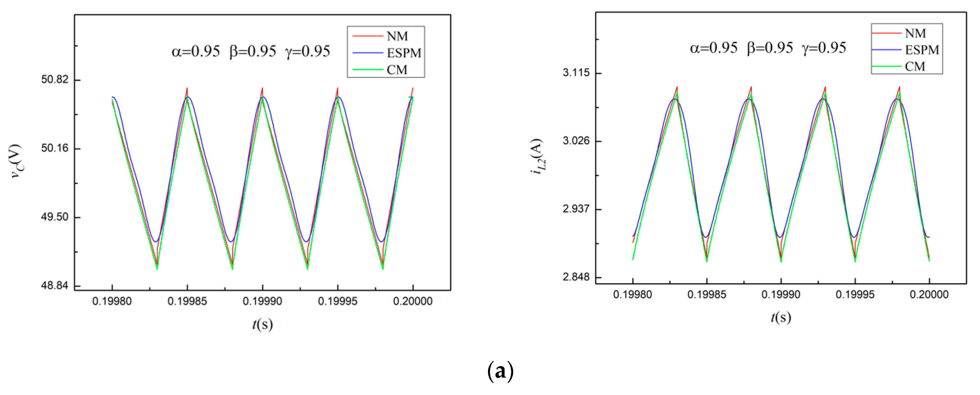
(2) Being different from the state space averaging method based on fractional calculus, the steady-state solutions of the fractional-order converter can be obtained by using the ESPM without considering the complex definition of fractional calculus. The simulation results of ESPM, NM, and CM are highly consistent. However, with the decrease of order, the relative errors of the ripple currents obtained from the ESPM model decrease most obviously, which make it suitable for modeling the Cuk converter with low orders. Moreover, the ESPM has the fastest simulation speed with flexibility and convenience of parameter adjustment.

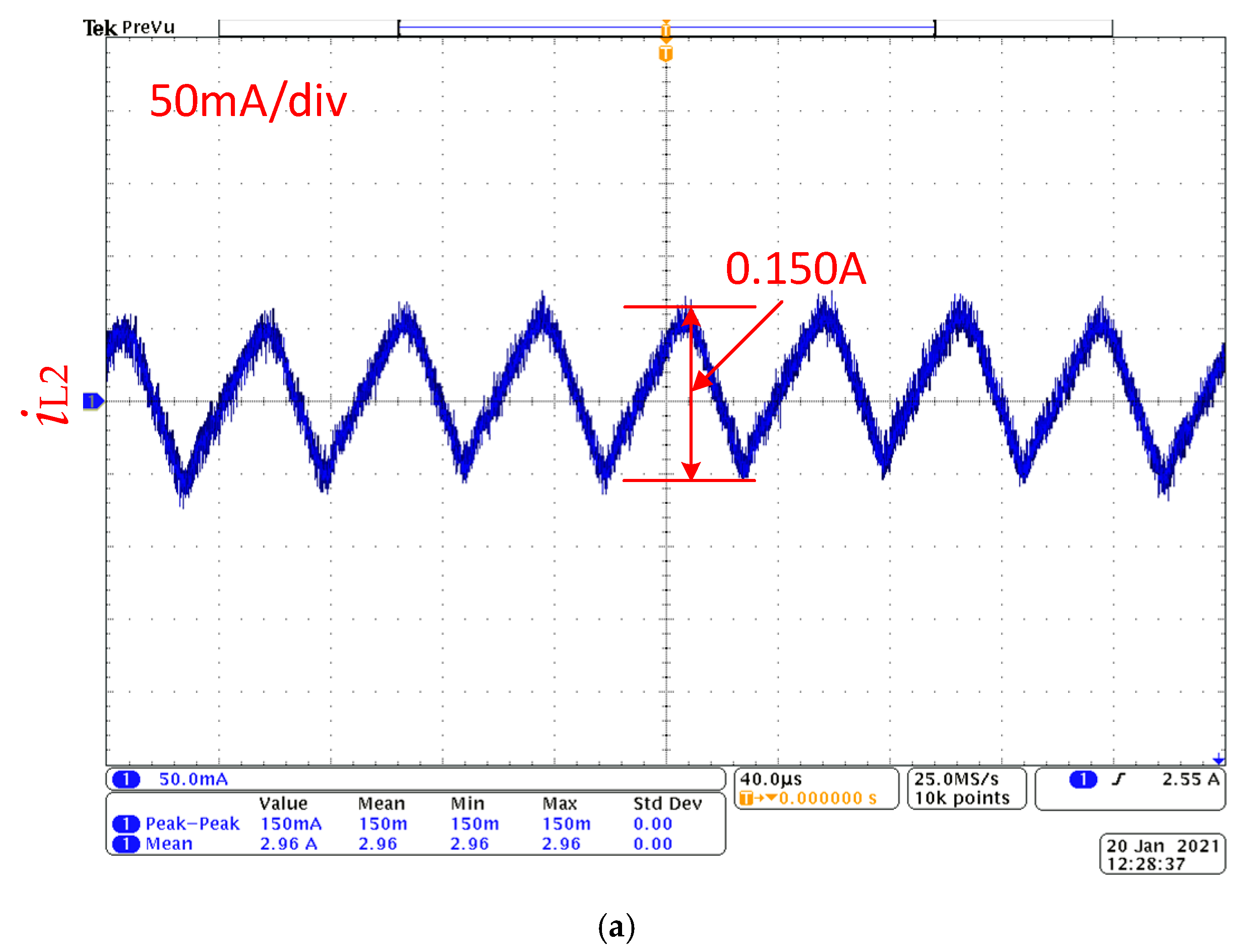
(3) The fractional-order Cuk converter based on circuit model is tested through hardware-in-the-loop experiment, which verifies the effectiveness of fractance chain construction based on Oustaloup filtering principle.

References

1. Westerlund, S.; Ekstam, L. Capacitor theory. IEEE Trans. Dielectr. Electr. Insul. 1994, 1, 826–839. [Google Scholar] [CrossRef]
2. Mandelbrot, B.B. The Fractal Geometry of Nature; WH Freeman: New York, NY, USA, 1982; pp. 1–10. [Google Scholar]
3. Charef, A.; Sun, H.H.; Tsao, Y.Y.; Onaral, B. Fractal system as represented by singularity function. IEEE Trans. Autom. Control 1992, 37, 1465–1470. [Google Scholar] [CrossRef]
4. Monje, C.A.; Chen, Y.; Vinagre, B.M.; Feliu-Batlle, V. Fractional-Order Systems and Controls: Fundamentals and Applications; Springer: London, UK, 2010; pp. 9–34. [Google Scholar]
5. Caponetto, R.; Dongola, G.; Fortuna, L.; Petráš, I. Fractional Order Systems: Modeling and Control Applications; World Scientific Publishing Co. Pte. Ltd.: Singapore, 2010; pp. 1–30. [Google Scholar]
6. Qiu, S.S.; Filanovsky, I.M. Harmonic analysis of PWM converters. IEEE Trans. Circuits Syst. I Fundam. Theory Appl. 2000, 47, 1340–1349. [Google Scholar]
7. Podlubny, I. Geometric and physical interpretation of fractional integration and fractional differentiation. Fract. Calc. Appl. Anal. 2002, 5, 367–386. [Google Scholar]
8. Chen, Y.Q.; Petras, I.; Xue, D.Y. Fractional order control-a tutorial. In Proceedings of the 2009 American Control Conference, St. Louis, MO, USA, 10–12 June 2009; pp. 1397–1411. [Google Scholar]
9. Hartley, T.T.; Lorenzo, C.F.; Qammer, H.K. Chaos in a fractional order Chua’s system. IEEE Trans. Circuits Syst. I Fundam. Theory Appl. 1995, 42, 485–490. [Google Scholar] [CrossRef]
10. Xie, H.; Liao, F.C.; Chen, Y.N.; Zhang, X.Y.; Li, M.L.; Deng, J.M. Finite-time bounded tracking control for fractional-order systems. IEEE Access 2021, 9, 11014–11023. [Google Scholar] [CrossRef]
11. Cao, J.Y.; Liang, J.; Cao, B.G. Optimization of fractional order PID controllers based on genetic algorithms. In Proceedings of the 2005 International Conference on Machine Learning and Cybernetics, Guangzhou, China, 18–21 August 2005; pp. 5686–5689. [Google Scholar]
12. Maiti, D.; Acharya, A.; Chakraborty, M.; Konar, A.; Janarthanan, R. Tuning PID and PIλDδ controllers using the integral time absolute error criterion. In Proceedings of the 2008 4th International Conference on Information and Automation for Sustainability, Colombo, Sri Lanka, 12–14 December 2008; pp. 457–462. [Google Scholar]
13. Barkas, D.A.; Ioannidis, G.C.; Psomopoulos, C.S.; Kaminaris, S.D.; Vokas, G.A. DC motor drives for industrial and automobile applications with emphasis on control techniques: A comprehensive review. Electronics 2020, 9, 887. [Google Scholar] [CrossRef]
14. Surya, S.; Williamson, S. Generalized circuit averaging technique for two-switch PWM DC-DC converters in CCM. Electronics 2020, 9, 1544. [Google Scholar]
15. Wu, C.; Si, G.; Zhang, Y.; Yang, N. The fractional-order state-space averaging modeling of the buck–boost DC/DC converter in discontinuous conduction mode and the performance analysis. Nonlinear Dyn. 2015, 79, 689–703. [Google Scholar] [CrossRef]
16. Chen, X.; Chen, Y.; Zhang, B.; Qiu, D.Y. A modeling and analysis method for fractional-order DC-DC converters. IEEE Trans. Power Electron. 2016, 32, 7034–7044. [Google Scholar] [CrossRef]
17. Fang, S.C.; Wang, X.G. Modeling and analysis method of fractional-order buck–boost converter. Int. J. Circ. Theor. Appl. 2020, 48, 1493–1510. [Google Scholar] [CrossRef]
18. Arackel, C.; Patil, M.D.; Vyawahare, V.; Raorane, A. Analysis of DC-DC Buck converter with lossy filter using fractional-order models. In Proceedings of the 2017 International Conference on Nascent Technologies in Engineering (ICNTE), Navi Mumbai, India, 1–5 January 2017. [Google Scholar]
19. Wang, F.Q.; Ma, X.K. Fractional order modeling and simulation analysis of boost converter in continuous conduction mode operation. Sci. Sin. 2011, 60, 070506. [Google Scholar]
20. Chen, Y.F.; Chen, X.; Hu, J.; Zhang, B.; Qiu, D.Y. A symbolic analysis method for fractional-order boost converter in discontinuous conduction mode. In Proceedings of the IECON 2017—43rd Annual Conference of the IEEE Industrial Electronics Society, Beijing, China, 29 October–1 November 2017; pp. 8738–8743. [Google Scholar]
21. Jia, Z.R.; Liu, C.X. Fractional-order modeling and simulation of magnetic coupled boost converter in continuous conduction mode. Int. J. Bifurcat. Chaos 2018, 28, 1850061. [Google Scholar] [CrossRef]
22. Matar, M.M.; Abbas, M.; Alzabut, J.; Kaabar, M.K.A.; Etemad, S.; Rezapour, S. Investigation of the p-Laplacian nonperiodic nonlinear boundary value problem via generalized Caputo fractional derivatives. Adv. Differ. Equ. 2021, 1, 68. [Google Scholar] [CrossRef]
23. Yang, C.; Xie, F.; Chen, Y.; Xiao, W.; Zhang, B. Modeling and analysis of the fractional-order Flyback converter in continuous conduction mode by Caputo fractional calculus. Electronics 2020, 9, 1544. [Google Scholar] [CrossRef]
24. Xie, L.; Liu, Z.; Zhang, B. A modeling and analysis method for CCM fractional order Buck-Boost converter by using R–L fractional definition. J. Electr. Eng. Technol. 2020, 15, 1651–1661. [Google Scholar] [CrossRef]
25. Matar, M.M.; Abu-Khamsin, S.A.; Hossain, M.E.; Mustapha, K. Analysis of subdiffusion in disordered and fractured media using a Grünwald-Letnikov fractional calculus model. Comput. Geosci. 2018, 22, 1231–1250. [Google Scholar]
26. Yang, R.; Liao, X.; Lin, D.; Dong, L. Modeling and analysis of fractional order Buck converter using Caputo–Fabrizio derivative. Energy Rep. 2020, 6, 440–445. [Google Scholar] [CrossRef]
27. Wen, D.R.; Chen, Y.F.; Zhang, B.; Qiu, D.Y.; Xie, F. Transient analysis of ZCS PWM converter based on equivalent small parameter method. IEEE J. Emerg. Sel. Top. Power Electron. 2020. early access. [Google Scholar] [CrossRef]
28. Chandrasekar, B.; Nallaperumal, C.; Dash, S. A nonisolated three-port DC–DC converter with continuous input and output currents based on Cuk topology for PV/fuel cell applications. Electronics 2019, 8, 214. [Google Scholar] [CrossRef] [Green Version]
29. Hanif, O.; Rayeen, Z.; Tiwari, S. Design and comparative analysis of fractional order controllers for Cuk converters. In Proceedings of the 2018 IEEE 8th Power India International Conference (PIICON), Kurukshetra, India, 1–6 December 2018. [Google Scholar]
30. Tiwari, S.; Rayeen, Z.; Hanif, O. Design and analysis of fractional order PID controller tuning via genetic algorithm for Cuk converter. In Proceedings of the 2018 IEEE 13th International Conference on Industrial and Information Systems (ICIIS), Rupnagar, India, 1–2 December 2018; pp. 436–441. [Google Scholar]
31. Duan, J.S.; An, J.Y.; Xu, M.Y. Solution of system of fractional differential equations by Adomian decomposition method. Appl. Math. 2007, 22, 7–12. [Google Scholar] [CrossRef]
32. Oustaloup, A.; Levron, F.; Mathieu, B.; Nanot, F.M. Frequency-band complex noninteger differentiator: Characterization and synthesis. IEEE Trans. Circuits Syst. I Fundam. Theory Appl. 2000, 47, 25–39. [Google Scholar] [CrossRef]
Figure 1. Cuk converter.
Electronics 10 00710 g001
Figure 2. Two modes of Cuk converter: (a) State 1; (b) State 2.
Electronics 10 00710 g002
Figure 3. Numerical model of the Cuk converter.
Electronics 10 00710 g003
Figure 4. Fractance chain circuit of the fractional-order inductor.
Electronics 10 00710 g004
Figure 5. Fractance chain circuit of the fractional-order capacitor.
Electronics 10 00710 g005
Figure 6. Circuit model of the Cuk converter.
Electronics 10 00710 g006
Figure 7. Capacitor voltages and inductor currents: (a) (α, β, γ) = (0.95, 0.95, 0.95); (b) (α, β, γ) = (0.9, 0.9, 0.9); (c) (α, β, γ) = (0.8, 0.8, 0.8); (d) (α, β, γ) = (0.8, 0.8, 0.9).
Electronics 10 00710 g007aElectronics 10 00710 g007b
Figure 8. Relative errors of Δ i L 2 .
Electronics 10 00710 g008
Figure 9. Effective values of the harmonic components of v C .
Electronics 10 00710 g009
Figure 10. Effective values of the harmonic components of i L 2 .
Electronics 10 00710 g010
Figure 11. Experimental environment.
Electronics 10 00710 g011
Figure 12. Experimental results: (a) i L 2 waveform of the integer-order Cuk converter; (b) i L 2 waveform of the 0.9-order Cuk converter.
Electronics 10 00710 g012aElectronics 10 00710 g012b