A Novel Interconnection Network with Improved Network Cost Through Shuffle-Exchange Permutation Graph

Abstract

The interconnection network represents an interconnected structure of processors that strongly determines the performance quality of a parallel processing system. The shuffle-exchange permutation (SEP) network with three degrees has high fault tolerance and can be efficiently simulated through star, bubble-sort, and pancake graphs. This study proposes a new interconnection network: the new SEP (NSEP), which improves the diameter and reduces network cost by adding one edge to the SEP network, and presents its graph properties and routing algorithms. The NSEP network, with a degree of connectivity of four, demonstrated maximum fault tolerance and Hamiltonian cycle. Furthermore, the diameter was seen to be improved by 40% or more and the network cost by 20% or more.

1. Introduction

With the explosive increase in data size owing to the recent advancements in information technology, the demand for high-performance computers with large computational power is increasing, particularly for big data and artificial intelligence applications. In response to these demands, high-performance computers with various computational processing units, such as graphics processing units (GPUs) and multicore processors, in addition to the conventional central processing units (CPUs), have been developed. Such computers are constantly evolving in response to new demands and requirements [1].

A parallel computer is a computer system that divides a given task and processes tasks among processing units operating in parallel. Parallel computers are classified into shared memory multiprocessors and message-passing multicomputers [2]. In the former, the memory system affects the overall system performance [3]. The interconnection network refers to the location and connection structure between processors and is one of the factors that determine the performance of a parallel processing system [4]. Hence, continuous research on interconnection networks is required to improve the performance of parallel processing computers.

Network cost is one of the measures of interconnection networks and is represented by the product of the number of degrees and the diameter. The number of degrees is related to the hardware cost and the diameter to the software cost. The network cost may be reduced by reducing the number of degrees or the diameter. The number of degrees is inversely correlated to the diameter. It is difficult to reduce the network cost because reducing the number of degrees increases the diameter, whereas reducing the diameter increases the number of degrees [4].

The interconnection networks mesh the hypercube and star graph classes depending on the number of nodes. The SEP [5] network is a star graph class with $n!$ nodes, with node and edge symmetry, has excellent scalability through recursive structures, and has a very small number of degrees and diameters over hypercube [6,7,8]. The existing SEP network has a maximum fault tolerance with a degree of connectivity of three, and efficient simulation can be performed for star, bubble sort, and pancake graphs. Thus, one can still get the advantage of the fixed degree of the network (independent of the size) [5]. In addition, NSEP networks with increased degree one also predict that simulation will be efficient for star, bubble sort, and pancake graphs.

For n-dimensional NSEP proposed in this study, when $n=2k$, the distance between two nodes, $\frac{n}{2}$, was reduced to one by adding an edge to the SEP. The proposed NSEP has a fixed number of degrees of four and has the properties of the existing SEP. The NSEP network has a maximum fault tolerance with a degree of connectivity of four and has a Hamilton cycle. Compared to the SEP network, the diameter was improved by more than 40% and the network cost by more than 20%.

In Section 2, we examine the network measure of the interconnection network, a constant-degree graph. In Section 3, we define the new interconnection network, $NSE{P}_n$, present the theoretical properties of graph and routing algorithm, and analyze the diameter. Finally, Section 4 concludes this study.

2. Related Works

In this chapter, we first consider the importance of the network measure and the advantages of the fixed number of degrees. Next, we examine the Hamiltonian cycle and SEP with an improved network cost.

In a multiprocessor system, a connected network for supporting the communication between each processor is called a multiprocessor interconnection network [9]. The interconnection network can be represented as an undirected graph representing each processor as a node and a communication link between processors as an edge. An edge is placed between any two processors with a link between them. This edge is an undirected edge that can bidirectionally transmit data. The interconnection network of parallel computers is represented as an undirected graph as follows:

$$G=\left(V,E\right)$$

where $V\left(G\right)$ is the set of nodes of graph G; that is, $V=\left\{0, 1, 2, \cdots , N-1\right\}$ and $E\left(G\right)$ is the set of edges of graph $G$. The edge of graph $G$ is a pair of arbitrary two nodes,$v$ and$w$ of $V\left(G\right)$. The necessary and sufficient condition for the existence of an edge$\left(v, w\right)$ is the presence of a communication link between nodes$v$ and$w$ [10,11,12,13,14,15].

Network measures for evaluating interconnection networks include number of degrees, diameter, network cost, connectivity, fault tolerance, and symmetry [10,15]. The number of degrees for a node$v$ refers to the number of edges adjacent to the node$v$, and the number of degrees for graph$G$ refers to the maximum value among the number of degrees of the nodes belonging to $V\left(G\right)$. A network that has an equal number of degrees for all nodes in graph $G$ is called a regular network. The diameter is the maximum value of the shortest path between any two nodes in the network and is the lower limit of the delay time required to transmit information to the entire network. A network having a relatively small diameter compared to the number of nodes, despite the short distance between nodes, has a disadvantage that it is difficult to design the network in terms of hardware as the number of nodes increases [16,17,18]. The interconnection networks that have been proposed until now can be classified into the following three types according to the number of nodes: mesh class with $k\times n$ nodes, hypercube class with $2^n$ nodes, and star graph class with$n!$ nodes [6].

The mesh structure has been widely used as a planar graph to date, and commercialized in various systems [19,20]. An m-dimensional mesh $M_m\left(N\right)$ consists of $N^m$ nodes and $m{N}^m-m{N}^{m-1}$ edges. Each node’s address is represented by an m-dimensional vector, and when the addresses of any two nodes differ by one in one dimension, there is an edge between them. Because low-dimensional meshes are easy to design and are useful from the algorithmic viewpoint, they are widely used as a network of parallel processing computers. The higher the dimension of a mesh, the smaller its diameter and the larger the bisection width, and various parallel algorithms can be rapidly executed; however, it is costly [6]. Structures that improve the diameter of a mesh with a typical lattice structure, hexagonal mesh, toroidal mesh, diagonal mesh, honeycomb mesh, and torus have been proposed [19,21].

The Hamiltonian path of the interconnection network is a path that passes through all nodes of $G$ only once. The Hamiltonian cycle of the graph$G$ refers to a path with the same starting and destination nodes as the path that passes through all nodes only once. If the network has a Hamiltonian path or Hamiltonian cycle, a ring or a linear array can be easily implemented, which can be utilized as a useful pipeline for parallel processing [22]. If the graph $v$ contains a Hamiltonian cycle, it is appropriate to include the Hamiltonian path.

The n-dimensional SEP graph $SE{P}_n$ is a regular network that represents nodes by permutation of each symbol and has three degrees [5]. In this respect, this study interchangeably uses nodes and permutation. There are three edges of $SE{P}_n-\left\{g_{12}, g_L, g_R\right\}$ according to the conditions. If an arbitrary node of $SE{P}_n$ is $S=s_1{s}_2{s}_3\cdots s_{n-1}{s}_n$, adjacent nodes are as follows.

• Edge $g_{12}$: Connects the nodes in which the leftmost first and the second symbols are exchanged in permutation. For example, it corresponds to a node $g_{12}\left(S\right)=s_2{s}_1{s}_3\cdots s_{n-1}{s}_n$ that is adjacent by an edge $g_{12}$ in a node $S$.
• Edge $g_L$: All symbols in the permutation are moved one digit to the left, and the leftmost symbol is moved to the rightmost position. For example, it corresponds to a node $g_L\left(S\right)=s_2{s}_3\cdots s_{n-1}{s}_n{s}_1$ that is adjacent by the edge $g_L$ in node $S$.
• Edge $g_R$: All symbols of the node permutation are moved to the right by one digit, and the rightmost symbol is moved to the leftmost position. For example, it corresponds to a node $g_R\left(S\right)=s_n{s}_1{s}_2{s}_3\cdots s_{n-1}$ that is adjacent by the edge $g_R$ in node$S$.

In node$S$, any node that is adjacent by edge operation $g_{12}$ is represented by $g_{12}\left(S\right)$, and the same method is applied to edge $\{g_L, g_R\}$. If the order of the edge sequence is $⟨g_L, g_{12}, g_R⟩$ when the edge operation is applied in the node$S$, the permutation change of this node is represented as $S$ → $g_L\left(S\right)$ → $g_{12}\left(g_L\left(S\right)\right)$ → $g_R(g_{12}\left(g_L\left(S\right)\right))$. The permutations of the node to which the edge sequence order $⟨g_L, g_{12}, g_R⟩$ is applied in the node $S$ are $S=s_1{s}_2{s}_3\cdots s_{n-1}{s}_n$, $g_L\left(S\right)=s_2{s}_3\cdots s_{n-1}{s}_n{s}_1$, $g_{12(}{g}_L\left(S\right)=s_3{s}_2\cdots s_{n-1}{s}_n{s}_1$, and $g_{R(}{g}_{12(}{g}_L\left(S\right)))=s_1{s}_3{s}_2\cdots s_{n-1}{s}_n$. Thus, when edge sequence $⟨g_L, g_{12}, g_R⟩$ is applied in node $S$, the last node is $g_{R(}{g}_{12(}{g}_L\left(S\right)=s_1{s}_3{s}_2\cdots s_{n-1}{s}_n$. Figure 1 shows a 4D $SE{P}_4$ graph.

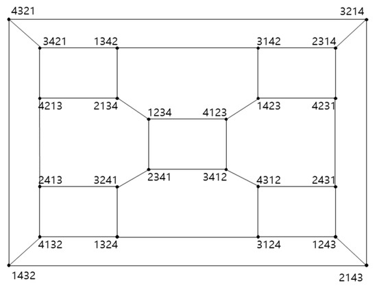
Figure 1. $SE{P}_4$ graph.

The SEP graph can be easily simulated on graphs based on permutation groups, such as a Cayley graph, and its algorithms can be efficiently executed in new graphs with minimal changes. The diameter of the SEP graph is $\frac{1}{8}\left(9n^2-22n+24\right)$, and its degree of connectivity is three, having a maximum fault tolerance [5]. Because $SE{P}_n$ is a Cayley graph, it has a node symmetric property [10]. The cycle, whose path length is $n$ and composed of edges $g_L$ (or $g_R$) in $SE{P}_n$, is called $s-cycle$ [5]. In the SEP graph, the positions of symbols are exchanged using edge operation $g_{12}$, and the symbol to be exchanged is moved to the leftmost position using edge operation $<g_L, g_R>$. This study improved the diameter value by adding one edge in which the symbol of the position $\frac{n}{2} + 1$ can be quickly moved to the leftmost position in the node permutation of the graph $SE{P}_n$.

3. Definition of New Interconnection Network NSEP_n and Routing Algorithm

3.1. Definition and Properties of NSEP_n Graph

The $NSE{P}_n\left(New-SE{P}_n\right)$ graph is a regular graph with four degrees obtained by adding one edge to the existing $SE{P}_n$ graph $\left(n=2k, k\ge 2\right)$. One edge added to $S=s_1{s}_2{s}_3\cdots s_{\frac{n}{2}}{s}_{\frac{n + 1}{2}}\cdots s_{n-1}{s}_n$, a node of $NSE{P}_n$, is an edge that connects the permutations in which the symbols $\frac{n}{2}$, $s_1~s_{\frac{n}{2}}$, and $s_{\frac{n + 1}{2}}~s_n$ have been exchanged. Let $g_{\frac{n}{2}}$ be an added edge of the $NSE{P}_n$ graph. The node is $g_{\frac{n}{2}}\left(s\right)=s_{\frac{n + 1}{2}}\cdots s_{n-1}{s}_n{s}_1{s}_2{s}_3\cdots s_{\frac{n}{2}}$ adjacent by the edge $g_{\frac{n}{2}}$ in the node $S=s_1{s}_2{s}_3\cdots s_{\frac{n}{2}}{s}_{\frac{n + 1}{2}}\cdots s_{n-1}{s}_n$. Therefore, the $NSE{P}_n$ graph has four edges $\left\{ g_{12}, g_L,g_R, g_{\frac{n}{2}}\right\}$ for each node. The four nodes $\left\{ g_{12}\left(S\right), g_L\left(S\right),g_R\left(S\right), g_{\frac{n}{2}}\left(S\right)\right\}$ adjacent to the node $S=s_1{s}_2{s}_3\cdots s_{\frac{n}{2}}{s}_{\frac{n + 1}{2}}\cdots s_{n-1}{s}_n$ of the $NSE{P}_n$ graph are shown below.

$$\begin{gathered} g_{12}\left(S\right)=\underset{\_}{s_2{s}_1}{s}_3\cdots s_{\frac{n}{2}}{s}_{\frac{n+1}{2}}\cdots s_{n-1}{s}_n \\ {g}_R\left(S\right)=\underset{\_}{s_n}{s}_1{s}_2{s}_3\cdots s_{\frac{n}{2}}{s}_{\frac{n + 1}{2}}\cdots s_{n-1} \\ {g}_L\left(S\right)=s_2{s}_3\cdots s_{\frac{n}{2}}{s}_{\frac{n + 1}{2}}\cdots s_{n-1}{s}_n\underset{\_}{s_1} \\ {g}_{\frac{n}{2}}\left(S\right)=\underset{\_}{\frac{s_{n+1}}{2}\cdots s_{n-1}{s}_n s_1{s}_2{s}_3\cdots s_{\frac{n}{2}}} \end{gathered}$$

Figure 2 shows an example of the $NSE{P}_4$ graph. In Figure 2, the thick line represents the edge $g_{12}$, the solid line represents the edge $g_L$ (or $g_R$), and the dotted line represents the edge $g_{\frac{4}{2}}\left(=g_{\frac{n}{2}}\right)$. For example, in the case of node 1234 in the $NSE{P}_4$ graph, adjacent nodes are $g_{12}\left(1234\right)=2134$, $g_L\left(1234\right)=2341$, $g_R\left(1234\right)=4123$, and $g_{\frac{4}{2}}\left(1234\right)=3412$.

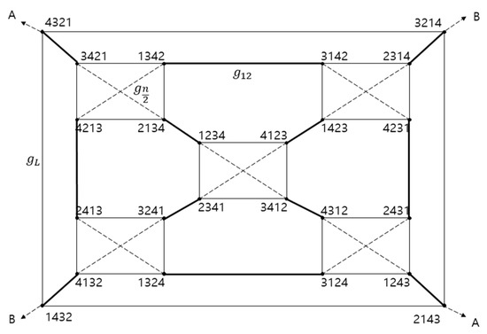
Figure 2. $NSE{P}_4$ graph.

Because the $NSE{P}_n$ graph has one extra edge over the $SE{P}_n$ graph, the latter is a subgraph of the former. Cycles whose path length is $n$ and which comprise the edges $g_L$ (or $g_R$) of the $NSE{P}_n$ are called s-cycles. For example, an s-cycle with the path length of four at the node S (= 1234) of $NSE{P}_4$ is

$$S=\left(1234\right)\stackrel{g_L}{\to }2341\stackrel{g_L}{\to }3412\stackrel{g_L}{\to }4123\stackrel{g_L}{\to }1234\left(=S\right)$$

A cluster in $NSE{P}_n$ has several important properties. These properties can be used to confirm that the $NSE{P}_n$ graph has a Hamiltonian cycle. The following definitions define the cluster and show its properties in Attributes 1, 2, and 3.

Definition 1.In the graph$NSE{P}_n$, a partial graph consisting of nodes constituting s-cycles and the edge$g_{\frac{n}{2}}$connecting the nodes in the s-cycles is called a graph$C_n$.

In $NSE{P}_4$, one cluster $C_4$ containing the node S (=1234) is a partial graph consisting of four edges $g_L$ (or $g_R$), and two edges $g_{\frac{n}{2}}$. Figure 3 shows $C_4$, the cluster of $NSE{P}_4$.

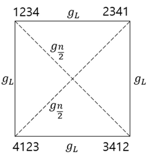
Figure 3. A cluster $C_4$.

Property 1.

There are $\left(n-1\right)!$ $C_n$ clusters in the $NSE{P}_n$ graph.

Proof. 

The total number of nodes in $NSE{P}_n$ is $n!$. A cluster $C_n$ is s-cycles with n different nodes and consists of $\frac{n}{2} g_{\frac{n}{2}}$ edges that connect nodes along the path constituting s-cycles. Moreover, the number of nodes in each cluster $C_n$ is n by s-cycles. Therefore, the number of $C_n$ clusters is $\frac{n!}{n}=\left(n-1\right)!$. □

Property 2.

The cluster $C_n$ of $NSE{P}_n$ has $\frac{n}{2} g_{\frac{n}{2}}$ edges.

Proof. 

There are n nodes in each cluster in the $NSE{P}_n$ graph, and they are adjacent to each other by $g_{\frac{n}{2}}$ edges that exchange $\frac{n}{2}$ symbols. Because there is only one node with such an adjacent relationship for one node, two nodes form a pair. Therefore, there are $\frac{n}{2} g_{\frac{n}{2}}$ edges connecting n nodes that constitute the cluster. □

Property 3.

A node $U$ constituting one cluster $C_n$ of $NSE{P}_n$ is adjacent to the node $g_{12}\left(U\right)$ of another cluster $C_n$ by the edge $g_{12}$. The n nodes constituting a cluster $C_n$ are adjacent to nodes of n different clusters $C_n$ by the edge $g_{12}$.

Proof. 

By the definition of $NSE{P}_n$ it can be seen that n nodes of a cluster C_n are adjacent to n nodes of different clusters $C_n$ by the edge $g_{12}$. □

Due to the added edge $g_{\frac{n}{2}}$, a new cycle with ($\frac{n}{2} + 1$) nodes exists. Definition 2 defines the cycles of $NSE{P}_n$ and the associated theorem is shown in Lemma 1, 2, and 3. In the Lemma 4, 5, and 6, we show that there is a Hamiltonian cycle between two adjacent nodes in cluster $C_n$ of NSEPn.

Definition 2.

When there is an arbitrary node$U$in the cluster$C_n$, let$V\left(=g_{\frac{n}{2}}\left(U\right)\right)$be the node$U$and the node adjacent to the edge$g_{\frac{n}{2}}$(however,$U\ne V$). Let the ($\frac{n}{2} + 1)$-cycle be the path from node$U$to the node$V$constituting the edge$g_L$(or$g_R$) at the path distance of$\frac{n}{2}$, and the path constituting the edge$g_{\frac{n}{2}}$at the node$U$.

Assume that there are nodes $U$( = 1234) and $V\left(=3412\right)$ at $NSE{P}_4$. The three-cycle path containing node $U\left(=1234\right)$ and $V\left(=3412\right)$ is given as $U\left(=1234\right)\stackrel{g_R}{\to }4123\stackrel{g_R}{\to }3412\left(=V\right)\stackrel{g_{\frac{4}{2}}}{\to }1234\left(=U\right)$.

Lemma 1.

When there is a node$U$in one cluster$C_n$, let$V\left(=g_{\frac{n}{2}}\left(U\right)\right)$be the node$U$and the node adjacent to the edge$g_{\frac{n}{2}}$(however,$U\ne V$). There are two ($\frac{n}{2} + 1)$-cycles that share the edge$g_{\frac{n}{2}}$connecting nodes$U$and$V$.

Proof. 

By Definition 2, ($\frac{n}{2} + 1)$-cycle is a path consisting of $g_{\frac{n}{2}}$ edge $g_R$ (or $g_L$), and 1 $g_{\frac{n}{2}}$ edge. It can be seen that these ($\frac{n}{2} + 1)$-cycles can create cycles using the edge $g_R$ and the edge $g_L$, respectively. Therefore, there are two ($\frac{n}{2} + 1)$-cycles that share the edge $g_{\frac{n}{2}}$. □

Lemma 2.

In each cluster of$NSE{P}_n$, there are$n$($\frac{n}{2}+1)$-cycles.

Proof. 

By Property 2, each cluster has $\frac{n}{2} g_{\frac{n}{2}}$ edges, and by Lemma 1, there are two ($\frac{n}{2}+1)$-cycles that share an edge $g_{\frac{n}{2}}$. Therefore, because $\frac{n}{2}\times 2=n$, there are $n$ ($\frac{n}{2}+1)$-cycles. □

Lemma 3.

The number of ($\frac{n}{2}+1)$-cycles in the network$NSE{P}_n$is$n!$.

Proof. 

By Lemma 2, there are n ($\frac{n}{2}+1$)-cycles in each cluster, and by Property 1, the number of $C_n$ clusters is $\left(n-1\right)!$. Therefore, the number of ($\frac{n}{2}+1)$-cycles in the $NSE{P}_n$ network is $\left(n-1\right)!\times n=n!$. □

Lemma 4.

There is a Hamiltonian path, whose path length is$n$, including an arbitrary node U in the cluster$C_n$, and a node$g_R\left(U\right)$(or$g_L\left(U\right)$) adjacent to the edge$g_R$(or g_L) from the node$U$.

Proof. 

Let $U$ be an arbitrary node of the cluster $C_n$. Let $V1\left(=g_L\left(U\right)\right)$ be the adjacent node by node $U$ and edge $g_L$, and the node adjacent by node and edge. Because each cluster $C_n$ has s-cycles of $NSE{P}_n$ as a partial graph, the path connected by node $U$ and edge $g_R$ (or $g_L$) has cycles including nodes $V1$ and $V2$. Therefore, there is a Hamiltonian cycle with the path length of $n$ from node $U$ to an adjacent node $V1\left(=g_L\left(U\right)\right)$ by an edge $g_L$, and an adjacent node $V2\left(=g_R\left(U\right)\right)$ by the node $U$ and the edge $g_R$. □

Lemma 5.

There is a Hamiltonian cycle between an arbitrary node$U$that constitutes a cluster$C_n$, and nodes$V1\left(=g_{\frac{n}{2}}\left(U\right)\right)$connected from the node$U$to the edge$g_{\frac{n}{2}}$.

Proof. 

Let $U$ be the starting node of the cluster $C_n$, and the target node$V1\left(=g_{\frac{n}{2}}\left(U\right)\right)$ be the node that is connected to node $U$ and the edge $g_{\frac{n}{2}}$. By the definition of $NSE{P}_n$ graph, the distance between the nodes $U$ and $V$ in s-cycles consisting of edges $g_L$ (or $g_R$) is $\frac{n}{2}$. Let $S1$ be a node at a $\left(\frac{n}{2}-1\right)$ distance along the s-cycle from the starting node $U$. The node $S2\left(=g_{\frac{n}{2}}\left(S1\right)\right)$ connected by the node $S2$, and the edge $g_{\frac{n}{2}}$ has a distance of $\frac{n}{2}$ in s-cycles. Therefore, node$S2$ is a node adjacent to $U$ located at a distance of $\left(\frac{n}{2}-1\right)$ from the node $S1$. A node at a $\left(\frac{n}{2}-1\right)$ distance along the s-cycle from a node$S2$ becomes a target node $V$. Because nodes $U$ and $V1\left(=g_{\frac{n}{2}}\left(U\right)\right)$ are adjacent to the edge $g_{\frac{n}{2}}$, a Hamiltonian cycle is formed. Therefore, there is a Hamiltonian cycle with a length $n$, connecting two adjacent nodes in the cluster $C_n$. □

Lemma 6.

There exists a Hamiltonian cycle that includes two adjacent nodes$U$,$V$in the cluster$C_n$.

Proof. 

By Lemmas 4 and 5, there is a Hamiltonian cycle that includes two adjacent nodes $U$, $V$ in the cluster $C_n$. □

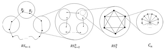
The reduced graph $R{S}_{n-1}$ of $NSE{P}_n$ represents the reduced s-cycles in $NSE{P}_n$ to one node. The node whose leftmost symbol is one in the permutation of n nodes constituting the s-cycles of $NSE{P}_n$ is called the leader node. The node address of the reduced graph $R{S}_{n-1}$ is represented by the remaining permutation addresses except one in the permutation of the leader node. In s-cycles 1234–4123–3412–2341, shown in Figure 4, the leader node is 1234, and s-cycle is represented by the super node 234 in the graph $R{S}_3$. Definition 3 defines a subgraph of $R{S}_{n-1}$ as $R{S}^k{}_{n-2}$ relative to the rightmost symbol. The theorem about it is shown in auxiliary Lemmas 7–9, and $NSE{P}_n$ shows that in Theorem 1 has a Hamilton cycle.

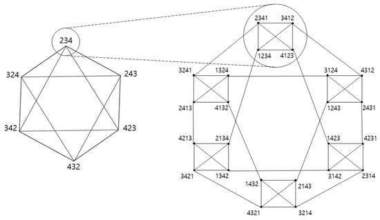
Figure 4. $R{S}_3$ and $NSE{P}_4$ graphs.

Definition 3.

A bubble-sort graph, which is a partial graph that includes all nodes of the reduced graph$R{S}_{n-1}$, is known as$RS{B}_{n-1}$. Furthermore,$RS{B}_{n-1}$is a$\left(n-2\right)$normal Cayley graph [5]. Therefore, when $R{S}_{n-1}$ is $n\ge 5$, it includes $n-1$ subgraph $R{S}_{n-2}$, and all $R{S}_{n-2}$ are adjacent to each other. Because the nodes belonging to $R{S}_{n-2}$ have the same rightmost symbol, when the rightmost symbol is k, the $R{S}_{n-2}$ of $R{S}_{n-1}$ is defined as $R{S}^k{}_{n-2}\left(2\le k\le n\right)$.

The $NSE{P}_n$ network has an even number of $n=2k$ symbols representing node addresses. In a network having an even number of symbols in $NSE{P}_n$, $R{S}_4$ does not exist. If $R{S}_{n-1}$ has a Hamiltonian cycle, it is natural that there is a Hamiltonian cycle when $n$ is even. After showing that there is a Hamiltonian cycle in $R{S}_{n-1}$, we show that there is also a Hamiltonian cycle in $NSE{P}_n$.

Lemma 7.

There is a Hamiltonian path between any two arbitrary nodes of$R{S}_3$, and it has a Hamiltonian cycle.

Proof. 

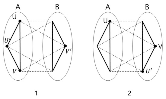
Let $U$ and $V$ be the starting and destination nodes, respectively.$R{S}_3$ can be divided into two areas A and B with the same number of nodes. The thick lines correspond to the edges within each area. There are three nodes constituting one area, and all nodes are adjacent. In addition, the nodes constituting the area have cycles in a complete graph, and there is always a Hamiltonian path between two nodes. In each node, there are two edges connecting to nodes in other areas. There are two cases of the relationship with nodes $U$ and $V$, as shown in Figure 5. The edges can be present in one area as shown in Figure 5-1, or in different areas as shown in Figure 5-2. Let $U^{\prime }\left(\ne V\right)$ and $V^{\prime }$ be a node adjacent to $U$ in area A and a node adjacent to $V$ in area B, respectively. There is a node adjacent to $U^{\prime }$ in area B, and there is a Hamiltonian path between this node and $V^{\prime }$. Therefore, in Case 1, there is a Hamiltonian path between $U$ and $V$. Now we move on to Case 2. Let $U^{\prime }\left(\ne V^{\prime }\right)$ be the node connected through the Hamiltonian path from $U$ in area A. Because both $U^{\prime }$ and $V$ are present in area B, there is a Hamiltonian path. That is, there is a Hamiltonian path between $U$ and $V$ in Case 2 as well. Therefore, because there is a Hamiltonian path between any two nodes of$R{S}_3$, and another Hamiltonian path between adjacent nodes, this has a Hamiltonian cycle. □

Figure 5. Areas A and B of $R{S}_3$.

Lemma 8.

If$C{N}_{n-1 }\left(n\ge 5\right)$isthe number of$R{S}_3$in$R{S}_{n-1}$,$C{N}_{n-1}=\frac{\left(n-1\right)!}{3!}$ is established.

Proof. 

By Definition 3, $R{S}_{n-1}$ has $n-1$ $R{S}_{n-2}$ subgraphs as a cluster. Figure 6 shows a subgraph on the RS_n-1. For example, if $n=5$, then $C{N}_4$, which is the number of $R{S}_3$ in $R{S}_4$ becomes $C{N}_4=C{N}_3\times 4$. Because $R{S}_{n-1}$ is hierarchical, let us assume $C{N}_{n-1}=C{N}_{n-2}\times \left(n-1\right)$. We prove that the formula $C{N}_{n-1}=\frac{\left(n-1\right)!}{3!}$ holds by mathematical induction. □

Figure 6. Relationship between $R{S}_{n-1}$ graph and subgraphs.

Because the number of $R{S}_3$ in $R{S}_3$ is 1, $C{N}_3=1$.

(i) When $n=5$, $C{N}_{n-1}=C{N}_{n-2}\times \left(n-1\right)=\frac{\left(n-1\right)!}{3!}$ holds.

This is true because $C{N}_4=C{N}_3\times 4=4$ and CN_{n − 1} = $\frac{\left(n-1\right)!}{3!}$ = $\frac{4!}{3!}$ = 4.

(ii) When $n=i$, it is assumed that $C{N}_{i-1}=\frac{\left(i-1\right)!}{3!}$ holds.

(iii) When $n=i+1$, we prove that it holds.

$$C{N}_{\left(i+1\right)-1}=C{N}_i=C{N}_{i-1}\times i=\frac{\left(i-1\right)!}{3!}\times i=\frac{\left(i-1\right)!\times i}{3!}=\frac{i!}{3!}=\frac{\left(\left(i+1\right)-1\right)!}{3!}$$

Therefore, the number of $R{S}_3$ in $R{S}_{n-1}$ satisfies the following equation.

$$C{N}_{n-1}=C{N}_{n-2}\times \left(n-1\right)=\frac{\left(n-1\right)!}{3!}$$

Lemma 9.

$R{S}_{n-1}$ has a Hamiltonian cycle.

Proof. 

By Definition 3, all $n-1$ $R{S}_{n-2}^k$ subgraphs are adjacent to each other in RS_{n − 1}. Let $R_i\left(1\le i\le \left(n - 1\right)!\right)$ and $R_j\left(1\le j\le \left(n-1\right)!, i\ne j\right)$ be any two nodes adjacent to each other in $R{S}_{n-1}$. Adjacent relationships are indicated by dotted lines. All nodes in $R{S}_{n-1}$ are adjacent to $R{S}_{n-2}^k$ through adjacent nodes. There is always adjacent $R{S}_{n-3}^k$ in $R{S}_{n-2}$. Therefore, it can be seen that $R{S}_3^k$ is always adjacent hierarchically in the same manner up to $R{S}_4$. As we have shown in Lemma 7, that there exists a Hamiltonian path between any two nodes, which implies that there exists a Hamiltonian cycle in $R{S}_{n-1}$. □

Theorem 1.

The$NSE{P}_n$network has a Hamiltonian cycle.

Proof. 

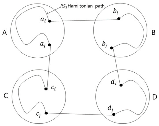
By Lemma 9, $R{S}_{n-1}$ has a Hamiltonian cycle, which regards the cluster $C_n$ of $NSE{P}_n$ as a super node. A node in an adjacent cluster of $NSE{P}_n$ is adjacent to another cluster through an adjacent node [5]. By Lemma 6, there is a Hamiltonian path between adjacent nodes of the cluster $C_n$. Thus, the $NSE{P}_n$ network has a Hamiltonian cycle. Figure 7 shows a Hamiltonian cycle of RS₄. □

Figure 7. Hamiltonian cycle of $R{S}_4$.

3.2. Routing Algorithm and Diameter Analysis

Routing refers to the path from one node to another. Because $SE{P}_n$ a partial graph of $NSE{P}_n$ is a Cayley graph, it is node symmetric [10]. Therefore, the path of the starting node $S$ and the destination node D can be regarded as the path of the starting node $S$ and the ID node. Let the ID node be $123\cdots n$. The algorithm proposed in this study is a method of placing the symbols in sequence up to n by iteratively applying the method of checking the positions of symbols 1 and 2, placing symbol 2 on the right side of symbol 1, and symbol 3 on the right side of symbol 2. The position of the symbol is represented in Definition 4, and the formulas used by the algorithm are represented in Lemmas 10–13.

Definition 4.

The position of the symbol$s_1$in the current node$S\left(=s_1{s}_2{s}_3\cdots s_i\cdots s_{n-1}{s}_n\right)$is represented by$p\left(s_i\right) \left(1\le i\le n\right)$.

In the case where the node address is 256,314 in $NSE{P}_6$, $p\left(1\right)=5$ and $p\left(2\right)=1$.

Lemma 10.

In node$S\left(=s_1{s}_2{s}_3\cdots s_i\cdots s_{n-1}{s}_n\right)$, the path of the node adjacent to the node by the edge sequence$⟨g_L, g_{12}, g_R⟩$is as follows. The last node permutation is$g_R\left(g_{12}\left(g_L\left(S\right)\right)\right)=s_1{s}_3{s}_2\cdots s_{n-1}{s}_n$in the path to which the edge sequence$⟨g_L, g_{12}, g_R⟩$is applied in node$S$. The path in node$S$is as given below.

$$\begin{gathered} S\left(=s_1{s}_2{s}_3\cdots s_i\cdots s_{n-1}{s}_n\right)\to g_L\left(S\right)=s_2{s}_3\cdots s_i\cdots s_{n-1}{s}_n{s}_1\to \\ g_{12}\left(g_L\left(S)\right)=s_3{s}_2\cdots s_i\cdots s_{n-1}{s}_n{s}_1\to g_R (g_{12}\left(g_L\left(S\right)\right)\right)=s_1{s}_3{s}_2\cdots s_i\cdots s_{n-1}{s}_n \end{gathered}$$

Lemma 11.

The number of iterations for an edge or edge sequence is denoted by$’\times \left[i\right]’$. For example, when$i=3$,$⟨g_A, g_B⟩\times \left[3\right]$=$⟨g_A, g_B⟩, ⟨g_A, g_B⟩, ⟨g_A, g_B⟩$. The number of iterations of the edge sequence is incorporated as given below.

$$⟨g_A, g_B⟩\times \left[i\right]$$

When $p\left(i\right)=a, p\left(i+1\right)=b$,

$$⟨g_A, g_B⟩\times \left[p\left(i\right)+p\left(i+1\right)-k\right]=⟨g_A, g_B⟩\times \left[a+b-k\right]$$

Lemma 12.

The value of the number of iterations of the edge sequence, which is less than 0, is subject to the reverse operation.

$$⟨g_A⟩\times \left[-n\right]= ⟨g_A^{-1}⟩\times \left[n\right]$$

Lemma 13.

The distance between the symbols$s_i$and$s_j$at the node address$S=s_1{s}_2{s}_3\cdots s_i\cdots s_j\cdots s_n \left(n=2^k, 1\le k\le lo{g}_{2}n\right)$is denoted by$\left|p\left(s_i\right)-p\left(s_j\right)\right|$.

The routing algorithm is outlined as follows.

[STEP 1] Symbol 2 is placed to the right of symbol 1. When the node address is divided by half, that is, $\frac{n}{2}$, the positions of the two symbols, $p\left(1\right)$ and $p\left(2\right)$ are checked, and the algorithm is executed according to the following cases. The cases are divided into the cases of $p\left(1\right), p\left(2\right)\le \frac{n}{2}$; $p\left(1\right), p\left(2\right)\ge \frac{n}{2}$; $p\left(1\right)\le \frac{n}{2} \mathrm{and} p\left(2\right)>\frac{n}{2}, \mathrm{or} p\left(2\right)\le \frac{n}{2} \mathrm{and} p\left(1\right)>\frac{n}{2}$.

[STEP 2] $i+1$ is placed to the right of symbol $i$. When the node address is divided by half, the positions of the two symbols, $p\left(i\right)$ and $p\left(i+1\right)$ are checked, and the algorithm is executed according to the following cases. The cases are divided into the cases of $p\left(i\right), p\left(i+1\right)\le \frac{n}{2}$, $p\left(i\right), p\left(i+1\right)>\frac{n}{2}$, and $\left( \left(p\left(i\right)\le \frac{n}{2} AND p\left(i+1\right)>\frac{n}{2}\right) OR \left(p\left(i+1\right)\le \frac{n}{2} AND p\left(i\right)>\frac{n}{2}\right) \right)$.

[STEP 3] In this algorithm, n is placed at the rightmost position while the relative positions from 1 to n are arranged in an ascending order, and this is the step of matching with the target node $ID$.

The routing shown in Algorithm 1.

Algorithm 1. Routing

[STEP 1] 1: case$p\left(1\right), p\left(2\right)\le \frac{n}{2}$ $2: \mathbf{if} (p\left(2\right)-p\left(1\right)=1) \mathrm{then} \mathrm{goto} [\mathrm{STEP} 2];$ $3: \mathbf{if} (p\left(1\right) !=1 AND p\left(2\right)!=1) \mathrm{then} \mathrm{exit} \mathrm{this} \mathbf{case} \mathrm{block}$ $4: \mathbf{if} ( k=2$$)⟨g_{12}⟩;$ 5:  else { $6: \mathbf{if} \left|p\left(2\right)-p\left(1\right)\right|=1$$) ⟨g_{12}⟩;$ $7: \mathbf{else} \{ ⟨g_{12}⟩$$, ⟨g_L, g_{12}⟩\times [\left|p\left(2\right)-p\left(1\right)\right|-2];$ $8: \mathbf{if} (p\left(2\right)<p\left(1\right)$$) ⟨g_L, g_{12}⟩;$ 9:   } 10:  } $11:⟨g_L, g_{12}⟩\times [\left|p\left(1\right)-p\left(2\right)\right|-1];$ $12:\mathbf{If} (p\left(2\right)<p\left(1\right)$$) ⟨g_L, g_{12}⟩;$ $13:\mathbf{case} p\left(1\right), p\left(2\right)>\frac{n}{2}$ $14: ⟨g_{\frac{n}{2}}⟩$ $15: \mathrm{goto} \mathrm{case} p\left(1\right), p\left(2\right)\le \frac{n}{2}$ $16:\mathbf{case} \left( \left(p\left(1\right)\le \frac{n}{2} AND p\left(2\right)>\frac{n}{2}\right) OR \left(p\left(2\right)\le \frac{n}{2} AND p\left(1\right)>\frac{n}{2}\right) \right)$ 17: Described in Appendix A. [STEP 2] $1:\mathbf{for} 1<i<n-1, \left(i=2, 3, \cdots , n-3, n-2\right) \{$ $2: \mathbf{case} p\left(i\right), p\left(i+1\right)\le \frac{n}{2}$ $3: \mathbf{if} (p\left(i+1\right)-p\left(i\right)=1 OR 1-n ) \mathrm{i}++;$ $4: \mathbf{elseif} (p\left(i\right)<p\left(i+1\right))\{$ $5: ⟨g_L⟩\times \left[p\left(i+1\right)-2\right], ⟨g_{12}⟩,<g_R, g_{12}>\times \left[p\left(i+1\right)-p\left(i\right)-2\right];\}$ $6: \mathbf{elseif} (p\left(i\right)>p\left(i+1\right))\{$ $7: ⟨g_{12}, g_L⟩\times \left[p\left(i\right)-p\left(i+1\right)-1\right], ⟨g_{12}⟩; \}$ $8: \mathbf{case} p\left(i\right), p\left(i+1\right)>\frac{n}{2}$ $9: ⟨g_{12}⟩$ $10: \mathrm{goto} \mathrm{case} p\left(i\right), p\left(i+1\right)\le \frac{n}{2} \}$ $11: \mathbf{case} \left( \left(p\left(i\right)\le \frac{n}{2} AND p\left(i+1\right)>\frac{n}{2}\right)OR \left(p\left(i+1\right)\le \frac{n}{2} AND p\left(i\right)>\frac{n}{2}\right) \right)$ 12:   Described in Appendix B. 13: } [STEP 3] $1:\mathbf{If} (p\left(n\right)<\frac{n}{2}-1$$) ⟨g_L⟩\times [p\left(n\right);$ $2:\mathbf{if} (p\left(n\right)=\frac{n}{2}-1$$) \{⟨g_R⟩$$, ⟨g_{\frac{n}{2}}⟩\};$ $3:\mathbf{if} (p\left(n\right)=\frac{n}{2}$$) ⟨g_{\frac{n}{2}}⟩;$ $4:\mathbf{if} (p\left(n\right)=\frac{n}{2}+1$$) \{⟨g_L⟩, ⟨g_{\frac{n}{2}}⟩\};$ $5:\mathbf{else} (p\left(n\right)>\frac{n}{2}+1$$) ⟨g_R⟩\times \left[n-p\left(n\right)\right];$

When the Algorithm 1 proposed in this study is applied, the process of sorting from nodes 2143 to 1234 is described as given below when n = 4.

[STEP 1] 2143 $\underrightarrow{g_{12}}$ 1243

[STEP 2] 1243 $\underrightarrow{g_{\frac{4}{2}}}$ 4312 $\underrightarrow{g_{12}}$ 3412

[STEP 3] 3412 $\underrightarrow{g_{\frac{4}{2}}}$1234

Theorem 2.

The diameter of$NSE{P}_n$is$\frac{2}{3}{n}^2-\frac{3}{2}n+1 \left(n=2k, k\ge 2\right)$.

Proof. 

In the worst case in [STEP 1], the diameter is n.

$$\begin{gathered} \mathrm{Case} \left( \left(p\left(1\right)\le \frac{n}{2} AND p\left(2\right)>\frac{n}{2}\right) OR \left(p\left(2\right)\le \frac{n}{2} AND p\left(1\right)>\frac{n}{2}\right) \right) \\ \left|p\left(1\right)-p\left(2\right)\right|\le \frac{n}{2}, \mathrm{and} \mathrm{it} \mathrm{satisfies} \mathrm{the} \mathrm{following}. \\ p\left(n\right)⟨\min \left(p\left(1\right), p\left(2\right)\right) OR p\left(n\right)⟩max\left(p\left(1\right), p\left(2\right)\right) \end{gathered}$$

In this case, the algorithm is described as follows.

$$\begin{gathered} ⟨g_{\frac{n}{2}}⟩, ⟨g_L⟩\times \left[\max \left(p\left(1\right), p\left(2\right)\right)-\frac{n}{2}-2\right],<g_{12}>, \\ ⟨g_R, g_{12}⟩\times \left[\left|p\left(1\right)-p\left(2\right)\right|-2\right], ⟨g_R, g_{12}⟩ \end{gathered}$$

Because the worst case of $\max \left(p\left(1\right), p\left(2\right)\right)$ is $\frac{n}{2}+2$, $\left|p\left(1\right)-p\left(2\right)\right|=\frac{n}{2}$. Therefore, in the worst case, the distance value is described as follows.

$$1+\frac{n}{2}+2-\frac{n}{2}-2+1\times \left(\frac{n}{2}-2\right)+2=n$$

In [STEP 2], in the worst case, the diameter is $\frac{2}{3}{n}^2-3n+3$.

$$\mathrm{Case} \left(p\left(i\right)\le \frac{n}{2} AND p\left(i+1\right)>\frac{n}{2}\right) OR \left(p\left(i+1\right)\le \frac{n}{2} AND p\left(i\right)>\frac{n}{2}\right).$$

When $\left|p\left(i+1\right)-p\left(i\right)\right|\le \frac{n}{2} AND$ $p\left(i\right)<p\left(i+1\right)$, the algorithm is described as follows.

$$⟨g_{\frac{n}{2}}⟩, ⟨g_L⟩\times \left[p\left(i+1\right)-\frac{n}{2}-2\right], ⟨g_{12}⟩, ⟨g_R, g_{12}⟩\times [p\left(i+1\right)-p\left(i\right)-2$$

Because the worst case of $p\left(i+1\right)$ is $\frac{n}{2}+3$, $p\left(i+1\right)-p\left(i\right)= \frac{1}{3}n$. The result is obtained as follows.

$$1+\frac{n}{2}+3-\frac{n}{2}-2+1+2\times \left(\frac{1}{3}n-2\right)+2=\frac{2}{3}n-1$$

Because $1<i<n-1$ in STEP 2, it is iterated by $n-3$ times as follows.

$$\left(\frac{2}{3}n-1\right)\left(n-3\right)=\frac{2}{3}{n}^2-3n+3$$

In the worst case in STEP 3, the diameter is $\frac{n}{2}-2$. The worst case is $p\left(n\right)<\frac{n}{2}-1$, and the algorithm is described as follows.

$$⟨g_L⟩\times \left[p\left(n\right)\right]$$

Therefore, in STEP 3, the worst case is $\frac{n}{2}-2$.

As a result, it can be seen that the diameter in the worst case of [STEP 1, 2, 3] is $\frac{2}{3}{n}^2-\frac{3}{2}n+1$ or less.

$$\mathrm{n}+\frac{2}{3}{n}^2-3n+3+\frac{n}{2}-2=\frac{2}{3}{n}^2-\frac{3}{2}n+1.$$

 □

For example, when $n=6$, in the worst case, the length is 16 as follows.

$$\begin{gathered} 253,164 \stackrel{g_{\frac{n}{2}}}{\to } 164,253 \stackrel{g_L^{-1}}{\to } 316,425 \stackrel{g_{12}}{\to } 136,425 \stackrel{g_R}{\to } 513,642 \stackrel{g_{12}}{\to } 153,642 \stackrel{g_R}{\to } 215,364 \stackrel{g_{12}}{\to } 125,364 \stackrel{g_{\frac{n}{2}}}{\to } 364,125 \stackrel{g_L^{-1}}{\to } 536,412 \stackrel{g_{12}}{\to } 356,412 \stackrel{g_{\frac{n}{2}}}{\to } 412,356 \stackrel{g_L^{-1}}{\to } \\ 641,235\stackrel{g_{12}}{\to } 461,235 \stackrel{g_R}{\to } 546,123 \stackrel{g_{12}}{\to } 456,123 \stackrel{g_{\frac{n}{2}}}{\to } 123,456 \end{gathered}$$

Theorem 3.

The network cost of$NSE{P}_n$is$\frac{8}{3}{n}^2-\frac{3}{2}n+4$.

Proof. 

The network cost is represented by the degree number X diameter. The network cost of $NSE{P}_n$ is as follows.

$$4\left(\frac{2}{3}{n}^2-\frac{3}{2}n+1\right)=\frac{8}{3}{n}^2-\frac{3}{2}n+4.$$

 □

In Table 1, the network cost of $NSE{P}_n$ was compared with the constant branching class connections. $NSE{P}_n$ increases the number of nodes rapidly as n increases. Thus, some of the network costs for each network were rearranged in Table 2 when the number of nodes was equal, and the results were shown in Table 3 and Figure 8 as a graph. Here, the network cost of $NSE{P}_n$ is always less than that of $SE{P}_n$, and we can see that when it is $n>10$, the network cost of $NSE{P}_n$ is the smallest.

Table 1. Network cost comparison of NSEP with other fixed degree networks.

Network	Node Number	Degree	Diameter	Network Cost
Mesh	$k\times n$	4	$2\sqrt{n}$	$O\left(8\sqrt{n}\right)$
Honeycomb mesh	$6n^2$	3	$1.63\sqrt{n}$	$O\left(4.9\sqrt{n}\right)$
Torus	$k\times n$	4	$\sqrt{n}$	$O\left(4\sqrt{n}\right)$
SEP	$n!$	3	$\frac{1}{8}\left(9n^2-22n+24\right)$	$O\left(\frac{27}{8}{n}^2\right)$
NSEP	$n!$	4	$\frac{2}{3}{n}^2-\frac{3}{2}n+1$	$O\left(\frac{8}{3}{n}^2\right)$

Table 2. Network cost comparison between constant degrees class and NSEP.

	Network Costs					Number of Nodes
n	Mesh	Honeycomb	Torus	SEP	NSEP	Mesh	Honeycomb	Torus	SEP (NSEP)
4	16.00	9.78	8.00	30	22.67	16	96	16	24
5	17.89	10.93	8.94	52	40.67	25	150	25	120
6	19.60	11.98	9.80	81	64.00	36	216	36	720
7	21.17	12.94	10.58	117	92.67	49	294	49	5040
8	22.63	13.83	11.31	159	126.67	64	384	64	40,320
9	24.00	14.67	12.00	208	166.00	81	486	81	362,880
10	25.30	15.46	12.65	264	210.67	100	600	100	3,628,800
11	26.53	16.22	13.27	327	260.67	121	726	121	39,916,800
12	27.71	16.94	13.86	396	316.00	144	864	144	479,001,600
13	28.84	17.63	14.42	472	376.67	169	1014	169	6,227,020,800
14	29.93	18.30	14.97	555	442.67	196	1176	196	87,178,291,200
15	30.98	18.94	15.49	645	514.00	225	1350	225	1.30767 × 1012

Table 3. Comparison of network costs when number of nodes are equal.

Number of Nodes	Network Costs
	Mesh	Honeycomb	Torus	SEP	NSEP
24	17		8.94	30	22.67
120	26.53	10	13.2	52	40.67
720	14.5	16	20.7	81	64
5040	67.4	26.3	33.7	117	92.67
40,320	113.4	44.2	56.7	159	126.67
362,880	196.45	120.08	98.22	208	166
3,628,800	349.17	213.43	174.59	264	210.67
39,916,800	635.89	388.69	317.94	327	260.67

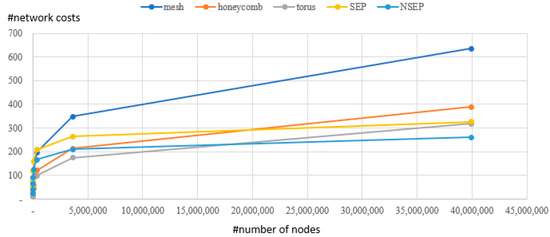
Figure 8. Network cost comparison when the number of nodes is the same.

In Figure 8, the five circles at the right end of the chart represent network costs of the mesh, honeycomb, SEP, torus, and NSEP, in that order from the top, when the number of nodes is 4 × 10⁸.

4. Conclusions

The SEP interconnection network has three degrees and a diameter of $\frac{1}{8}\left(9n^2-22n+24\right)$. This study proposed a new interconnection network NSEP by adding a new edge to the SEP network. In the NSEP network, the diameter and network cost were improved by reducing the distance between two nodes in a $\frac{n}{2}$ distance to one by adding one edge to the existing SEP network.

The $NSE{P}_n$ interconnection network proposed in this study has the same number of nodes as SEP, having four degrees, a diameter of $\frac{2}{3}{n}^2-\frac{3}{2}n+1$, and a network cost of $O\left(n^2\right)$. The interconnection network $NSE{P}_n$ shows excellent results by reducing the diameter by 40% or more and the network cost by 20% or more, while increasing the number of degrees by one in comparison to SEP. The interconnection network NSEP is a network with a Hamiltonian cycle and SEP as a subgraph. Because the NSEP network is defined to only have an even number of nodes (n = 2k), a generalized graph definition is additionally required. The algorithm designed in this paper is an algorithm that sorts symbols 1 through n. In some cases, the opposite arrangement of n through 1 may be effective. Further research will be required under conditions that allow us to select efficient algorithms between the two algorithms. It is hoped that this will lead to research on interconnected networks to improve the performance of parallel processing computers.

References

- Kim, N.-G. A Study on the Development of the Composite Measures of High-Performance Computer Technology; Sungkyunkwan University: Seoul, Korea, 2020. [Google Scholar]
- Dadheech, P.; Kumar, A. Fault-Tolerant Adaptive XY Routing for Multiprocessors in HPC Network. J. High Perform. Comput. 2020, 3, 94–118. [Google Scholar] [CrossRef]
- Culler, D.; Singh, J.P.; Gupta, A. Parallel Computer Architecture—A Hardware/Software Approach; Gulf Professional Publishing: Houston, TX, USA, 1999. [Google Scholar]
- Steller, P. A survey of the Degree/Diameter Problem for Undirected Graphs. Ph.D. Thesis, University of Delaware, Newark, NJ, USA, 2020; pp. 1–5. [Google Scholar]
- Latifi, S.; Srimani, P.K. A New Fixed Degree Regular Network for Parallel Processing; IEEE Computer Society Press: New York, NY, USA, 1996; pp. 152–159. [Google Scholar]
- Adhikari, N.; Singh, A. Leafycube: A Novel Hypercube Derivative for Parallel Systems. In Advances in Data Science and Management; Springer: Singapore, 2020; pp. 323–332. [Google Scholar]
- Gu, M.M.; Hao, R.X.; Tang, S.M.; Chang, J.M. Analysis on component connectivity of bubble-sort star graphs and burnt pancake graphs. Discret. Appl. Math. 2020, 279, 80–91. [Google Scholar] [CrossRef]
- Yeh, C.-H.; Varvarigos, E. Macro-Star Network: Efficient Low-Degree Alternatives to Star Graphs for Large-Scale Parallel Architectures. IEEE Trans. Parallel Distrib. Syst. 1996, 9, 987–1003. [Google Scholar]
- Gholizadeh, R.; Valinataj, M. Reliability Improvement of Fault-Tolerant Shuffle Exchange Interconnection Networks. In Proceedings of the 2020 10th International Conference on Computer and Knowledge Engineering (ICCKE), Mashhad, Iran, 29–30 October 2010; pp. 336–341. [Google Scholar]
- Akers, S.B.; Krishnamurthy, B. A group-theoretic model for symmetric interconnection networks. IEEE Trans. Comput. 2018, 38, 555–566. [Google Scholar] [CrossRef]
- Mnejja, S.; Aydi, Y.; Abid, M.; Monteleone, S.; Catania, V.; Palesi, M.; Patti, D. Delta multi-stage interconnection networks for scalable wireless on-chip communication. Electronics 2020, 9, 913. [Google Scholar] [CrossRef]
- Wu, H.I.; Tsay, R.S.; Chang, F.Y. CORONA: A k-COnnected RObust Interconnection Network Generation Algorithm. In Proceedings of the 2020 International Symposium on VLSI Design, Automation and Test (VLSI-DAT), Hsinchu, Taiwan, 10–13 August 2020. [Google Scholar]
- Mnejja, S.; Aydi, Y.; Abid, M.; Monteleone, S.; Catania, V.; Palesi, M.; Patti, D. Hierarchical and reconfigurable optical/electrical interconnection network for high-performance computing. IEEE/OSA J. Opt. Commun. Netw. 2020, 12, 50–61. [Google Scholar]
- Pai, K.-J. A Parallel Algorithm for Constructing Two Edge-Disjoint Hamiltonian Cycles in Crossed Cubes. In Proceedings of the International Conference on Algorithmic Applications in Management, Jinhua, China, 10–12 August 2020. [Google Scholar]
- Lakshmivarahan, S.; Jwo, J.S.; Dhall, S.K. Symmetry in interconnection networks based on cayley graphs of permutation groups: A survey. Parallel Comput. 1993, 19, 361–407. [Google Scholar] [CrossRef]
- Yasudo, R.; Nakano, K.; Koibuchi, M.; Matsutani, H.; Amano, H. Designing low-diameter interconnection networks with multi-ported host-switch graphs. Concurr. Comput. Pract. Exp. 2020, e6115. [Google Scholar] [CrossRef]
- Moudi, M.; Othman, M. A survey on emerging issues in interconnection networks. Int. J. Internet Technol. Secur. Trans. 2021, 11, 131. [Google Scholar] [CrossRef]
- Mahafzah, B.A.; Alshraideh, M.; Tahat, L.; Almasri, N. Topological Properties Assessment for Hyper Hexa-Cell Interconnection Network. Int. J. Comput. 2019, 13, 115–121. [Google Scholar]
- Bokka, V.H.; Gurla, S.; Olariu, J.L. Podality-based time-optimal computations on enhanced meshes. IEEE Trans. Parallel Distrib. Syst. 1997, 8, 1019–1035. [Google Scholar] [CrossRef]
- Ranade, A.G.; Johnsson, S.L. The Communication Efficiency of Meshes, Boolean Cubes and Cube Connected Cycles for Wafer Scale Integration; Thinking Machines Corporation: Waltham, MA, USA, 1987; pp. 479–482. [Google Scholar]
- Chen, J.L.; Shin, K.G. Addressing, routing, and broadcasting in hexagonal mesh multiprocessors. IEEE Trans. Comput. 1990, 39, 10–18. [Google Scholar] [CrossRef]
- Robin, J.W.; John, J.W. Graphs an Introductory Approach; John and Wiley and Sons: Hoboken, NJ, USA, 1990. [Google Scholar]
Publisher’s Note: MDPI stays neutral with regard to jurisdictional claims in published maps and institutional affiliations. |
© 2021 by the authors. Licensee MDPI, Basel, Switzerland. This article is an open access article distributed under the terms and conditions of the Creative Commons Attribution (CC BY) license (https://creativecommons.org/licenses/by/4.0/).