Abstract
The paper is concerned with designing an effective controller for a linear tubular homopolar (LT-H) motor type. The construction and operation of the LT-H motor are first described in detail. Then, the motor model is represented in the direct-quadrature (d-q) axes in order to facilitate the design of the control loops. The designed control system consists of two main loops: the current control loop and velocity adaptation loop. The determination of the regulator’s gains is accomplished through deriving and analyzing the transfer functions of the loops. To enhance the system’s robustness, a robust variable estimator is designed to observe the velocity and stator resistance. Different performance evaluation tests are performed using MATLAB/Simulink software to validate the controller’s robustness for variable-speed operation and load force changes as well. The obtained results reveal the appropriate dynamics of the motor thanks to the well-designed control system.
1. Introduction
The invention of linear motors dates back to about a century ago, about 50 years after the advent of rotating machines; however, their development and use were not very widespread due to difficulties with their construction techniques at that time. Only with technology improvements since the end of the 1970s (especially in high-speed-rail transport systems) has interest in the linear motor and its use increased [1,2].
Unlike traditional motors in which the developed motion is rotary, in linear drives, the motion is transmitted along a straight line, which represents the great advantage of this type, as it allows the elimination of mechanical transmission and increases the degree of reliability. Other characteristics of linear motors can be identified through their geometry: first of all, they have a beginning and an end in the direction of motion; this aspect manifests itself with an undesired effect called the edge effect. A second aspect that makes it particular is the presence of an air gap, which in some types reaches considerable dimensions, and precludes or prevents the possibility of obtaining high values of efficiency [3].
Finally, another peculiarity is represented by the presence of an attractive or repulsive force that manifests itself in a direction perpendicular to the direction of the motion, which in some applications (high-speed transport) is used to levitate the secondary with respect to the primary one.
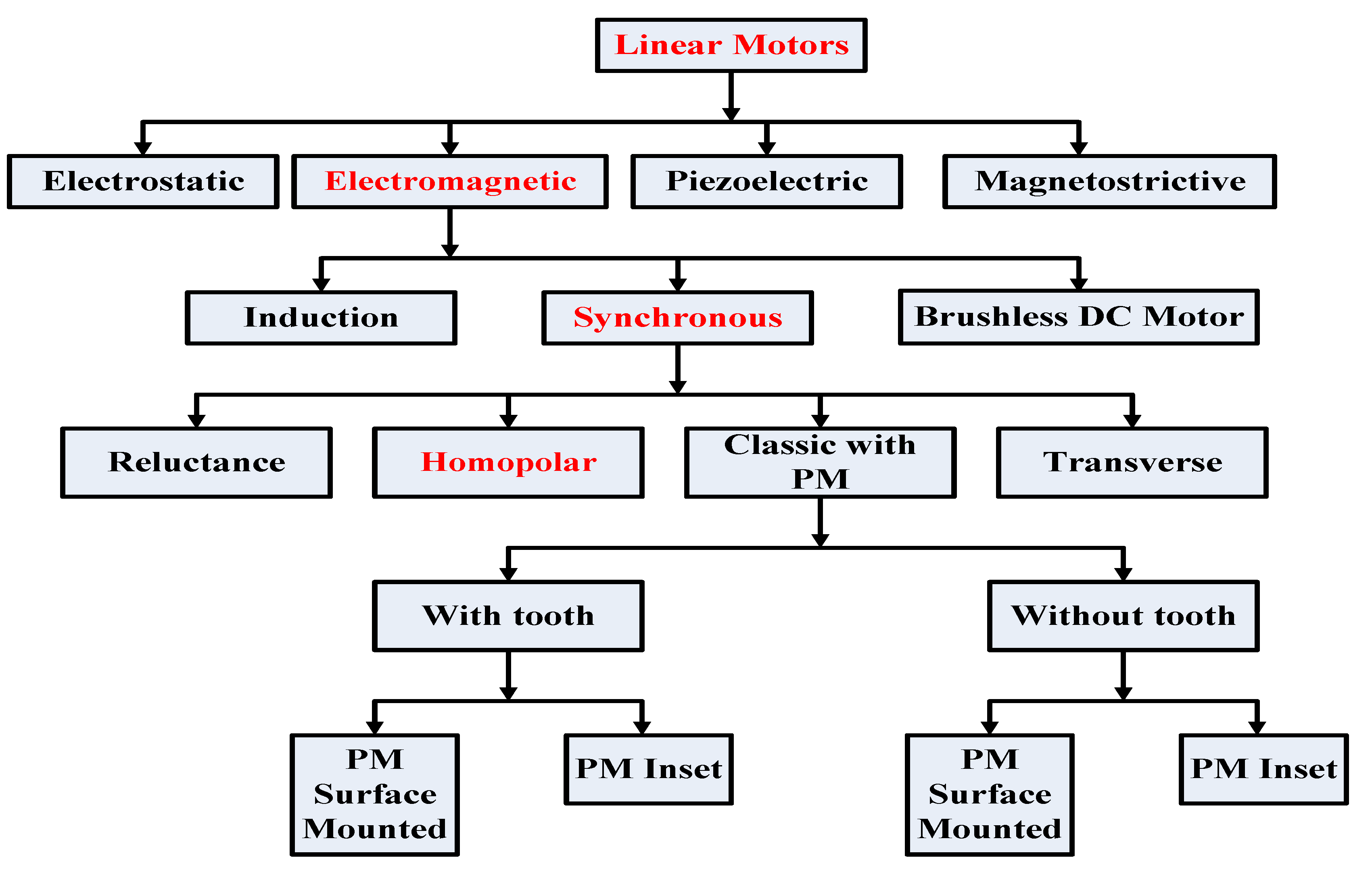
As for the rotary motor, the linear motor also has a considerable range of types that differ both in the principle of operation and from the construction point of view [4]: there are synchronous motors, indicated with the abbreviation LSM; induction (LIM); and transverse flow or longitudinal flow. According to the geometrical aspects, they are distinguished by the length of the fixed and movable parts, and they also can be single- or double-sided according to whether the structure embraces one or two sides of the machine. We can also distinguish the switched reluctance linear synchronous motor (SRLSM) and the permanent magnet linear synchronous motor (PMLSM), which have the characteristic of having windings on one side only, but the impossibility of having high magnetic fields (they are missing the excitation circuit), which does not allow them to provide high power. Figure 1 reports the possible classifications of the various types of linear motors, within which the linear tubular homopolar type is identified.

Figure 1.
Classifications of linear motors.
Linear motors give a realistic solution to several actuation needs. The presented study in [5] discussed different sorts of applications for which linear motors are suitable. Linear motors are utilized with plastic threads for textiles, and can position microscope tables and drive laser-photo exposure machines. These motors are available in several shapes, and the specific needs of the motor outline which type is best fitted to the application. They can be flat, tubular, rotary or convert rotation to linear translation.
Some tubular linear motors consist of pneumatic or hydraulic arms, which are suitable for applications that do not require high precision, but need a high force in a compact space. Hydraulic actuators are typically used in heavy equipment vehicles such as tractors, dump trucks and bulldozers. Hydraulics are consistent with these applications because hydraulic pumps can be powered freely from the drive-train of the engine and provide large power to the actuators. Hydraulics are a bit bulky and slow, and for these reasons they are not compatible with compact precision placement.
Pneumatic actuators provide high power density, but they are remarkably less accurate than electrical actuators. The study in [6] displayed some of the improvements that pneumatic motors have made, and presented a design for a rotary pneumatic motor that can accomplish some tasks initially performed only by rotating motors. The study in [7] used a combination of pneumatic and electric rotary motors to capitalize on the advantages of each.
Other linear motors utilize an electric rotary motor with a leadscrew or other linkage types to convert the rotary action to linear translation, as in [8]. However, the required mechanism to achieve the conversion causes serious complications in the system. These complications include backlash and heavy weight of the moving parts due to connecting gears or linkages. Regardless of these difficulties, leadscrew linear motors are usually used in high-precision manufacturing equipment, such as two-degree-of-freedom planar positioning used in metal-working mills.
Another application in which the LT-H motor type can be used is the reciprocating compressors of refrigerators. Until recently, most refrigeration apparatus used traditional rotary compressors, which consume large amounts of electricity. In practice, the reciprocating compressor utilizes mechanical tools; for example, a crank mechanism is used to convert the rotary motion to linear reciprocating motion in order to drive the piston. This crank mechanism generates remarkable friction losses. As a result, there are great challenges in improving the efficiency of rotary compressors, so new categories of compressors (e.g., linear compressors) have received much attention from many researchers [9,10,11,12,13,14]. The linear compressor has several merits over the traditional rotary one: it does not place any side load on the sliding bearings, no gearbox is required to be connected with the payload, and moreover, it is compact and more reliable [15,16,17,18]. Another application of the LT-H motor is the active-pedal system used in vehicles. An active-pedal system is a motorized systems that is mounted in a vehicle’s accelerator. Unlike the traditional mechanical pedal, it is typically rotated by an electric motor developing a vibration force opposing the drivers’ foot-press force [19].
Due to their enhanced dynamics compared with the rotary machines in specific applications as mentioned earlier, linear motors were given great concern from the designers to fulfill specific needs [20,21,22,23,24,25,26,27,28,29]. For example, in [20], the design of a transverse-flux linear tubular machine type was presented to harvest a higher force density; the finite element method (FEM) was utilized for this purpose. In [21], the characteristics of a linear tubular electromagnetic launcher were analyzed and optimized. The launcher used a linear tubular PMSM, and an FEM analysis was also utilized to test and validate the design. In [22], the electromagnetic parameters and static features of a linear tubular reluctance motor were determined for a sinusoidal motor excitation. In [23], a tubular-transverse flux linear motor was optimally designed in order to reduce the cogging force. In [24], the authors utilized the FEM method to optimally design a homopolar linear tubular motor via analyzing the magnetic motor circuit and its relevant magnetic behaviors. In [25], a linear tubular PM synchronous generator was designed and tested using a 3D FEM analysis.
The optimal design of linear motors is a vital task that must be correctly accomplished to achieve an effective operation. However, the control also plays a complementary role to the design. For this purpose, several articles have dealt with developing robust controllers for different types of linear motors [26,27,28,29]. In [26], a force-control system was constructed for a linear tubular motor used in the active-pedal system in vehicles. In [27], a nonlinear predictive controller was used for tracking the speed of a LIM. In [28], a thrust-control mechanism was developed for a LIM to achieve a stable operation and reduce the thrust deviation. In [29], a combined vector control and direct thrust-control system was utilized to manage the operation of a LIM while compensating for the end effect at the same time. In [30], a recursive adaptive controller was designed using the sliding-mode theory to manage the operation of a linear motor positioner. A stability analysis was introduced to confirm the zero-tracking-error operation. In [31], adaptive programming and neural networks were combined to formulate a nonlinear controller for a linear PMSM. Feedback linearization principles were adopted to enhance the system’s robustness against parameter change. In [32], a position controller for a linear PMSM was introduced, in which pole-placement theory was considered while adopting the online parameter estimation. All of these studies aimed to avoid the effects of system uncertainties. In [33], a combined predictive and adaptive internal (AI) controller was formulated to achieve a high-bandwidth current regulation for a linear PMSM. The time-delay compensation and bandwidth increase were realized using predictive control; meanwhile, the AI control was used to observe uncertainties such as parameter changes. In [34], a position-tracking controller was introduced for a linear PMSM. In this study, an improved PID controller was formulated by considering an upper limit of the lumped-model uncertainties and outer disturbances. In [35], a model for a predictive thrust force control for a double-sided linear vernier PMSM was introduced. In this study, two active voltages were selected during the prediction stage rather than using only one voltage vector, which helped in enhancing the control precision. Moreover, the cost function form used was much simpler compared with traditional forms due to the absence of weighting values.
Despite the improved dynamics that were obtained using these controllers, the lack of a thoroughly theoretical analysis for the used controllers was the main shortcoming. The detailed analysis and derivation of any control system is a requirement to illustrate when and why the controller works properly. This task can be accomplished via analyzing each internal closed control loop in the system. Moreover, the control of a linear tubular homopolar (LT-H) motor type is rare in the literature, and to investigate more about this type, the current paper introduces a detailed analysis for the control-system design of the LT-H motor type.
Sensorless operation is a desired requirement from the cost and reliability points of view. Different velocity estimators were introduced for different types of linear motors [36,37,38]. The study in [36] proposed an adaptive Luenberger neural-based observer for a LIM. The effectiveness of the observer was approved for different operating regimes, even though the most significant shortcoming was the observer’s complexity. In [37], the authors designed a flux observer for a linear vernier PMSM. The estimator consisted of a feedback controller and a disturbance observer. An appropriate performance was obtained from the observer, but the requirement of precise gain tuning made the observer quite complex. In [38], a sensorless scheme was introduced for a linear PMSM used in reciprocating-pump applications. The sensorless scheme was in the form of a Luenberger observer, which estimates the back-emf and extracts the speed from it. The introduced observer was very simple, but it lacked the ability to investigate the system’s robustness against disturbances and uncertainties such as resistance change. In [39], an extended Kalman filter (EKF) was adopted to observe the velocity of a linear flux-switching PMSM. The filter precisely tracked the variable changes, but a delayed system response was the main deficiency. In [40], a Kalman filter was designed by considering the phase-locked loop principle in order to estimate the speed of a LIM. The designed filter used a prefiltering unit and a magnitude-normalization tool in order to reject the disturbances and deal with parameter changes. Even though it achieved the appropriate observation, the system was obviously lacking in simplicity.
As an attempt to maintain the simplicity and robustness of the estimator, a robust observer is designed in the present study to estimate the velocity and stator resistance as well. The estimator’s operation depends on extracting and estimating the two variables via comparing two values of rotor back-electromotive forces (emfs) (actual and estimated quantities). The estimator design is explained in a systematic manner while clarifying the theoretical principles upon which it stands.
According to the previous review, the contributions that the current paper introduces to the literature can be itemized as follows:
- The paper introduces a detailed analysis for the modeling and control of a linear tubular homopolar (LT-H) motor.
- The paper investigates several operating regimes for the motor to test and validate the designed controller.
- The frequency response of the controller’s loops is presented to identify the most appropriate gains.
- An effective estimator is designed to achieve sensorless operation and reduce the system’s cost.
- The introduced systematic analysis enables the extension of the controller to be used by other linear motor types after considering the structure and model of each type.
The current paper is structured as follows: in Section 2, the mathematical model of the LT-H motor is introduced and analyzed in different coordinates; in Section 3, the design of the proposed controller is described; in Section 4, the design of the sensorless scheme is introduced; in Section 5, the performance tests are carried out and the results are analyzed; and finally, Section 6 presents the conclusions and outcomes of the study.
1.1. Motor’s Structure and Theory of Operation
The motor under study has a permanent magnet and three-phase stator windings inserted in the primary magnetic core; this arrangement produces an alternating magnetic field, which provides a translating magnetic field with a speed directly related to the amplitude of the resulting polar half-pass equal to the step between two salient points of the track (pole pitch).
The secondary instead is constituted by a cursor composed of a cylinder in which iron parts and parts of nonmagnetic material alternate in subsequence, which guarantees the presence of a variable reluctance along the development of the movement.
Therefore, the observed resultant force turns out to be the effect of two contributions caused by:
- The difference in reluctance between the various magnetic paths of the machine; and
- The Lorentz force on the stator windings.
The construction specifications state that the power supply is provided by a 220 V single-phase network through the presence of an inverter and a rectifier. This input stage must ensure that it impresses on each motor phase a voltage greater than 80 Vrms and a star-shaped voltage, which allows obtaining a good control of the motor, ensuring rapid accelerations and decelerations.
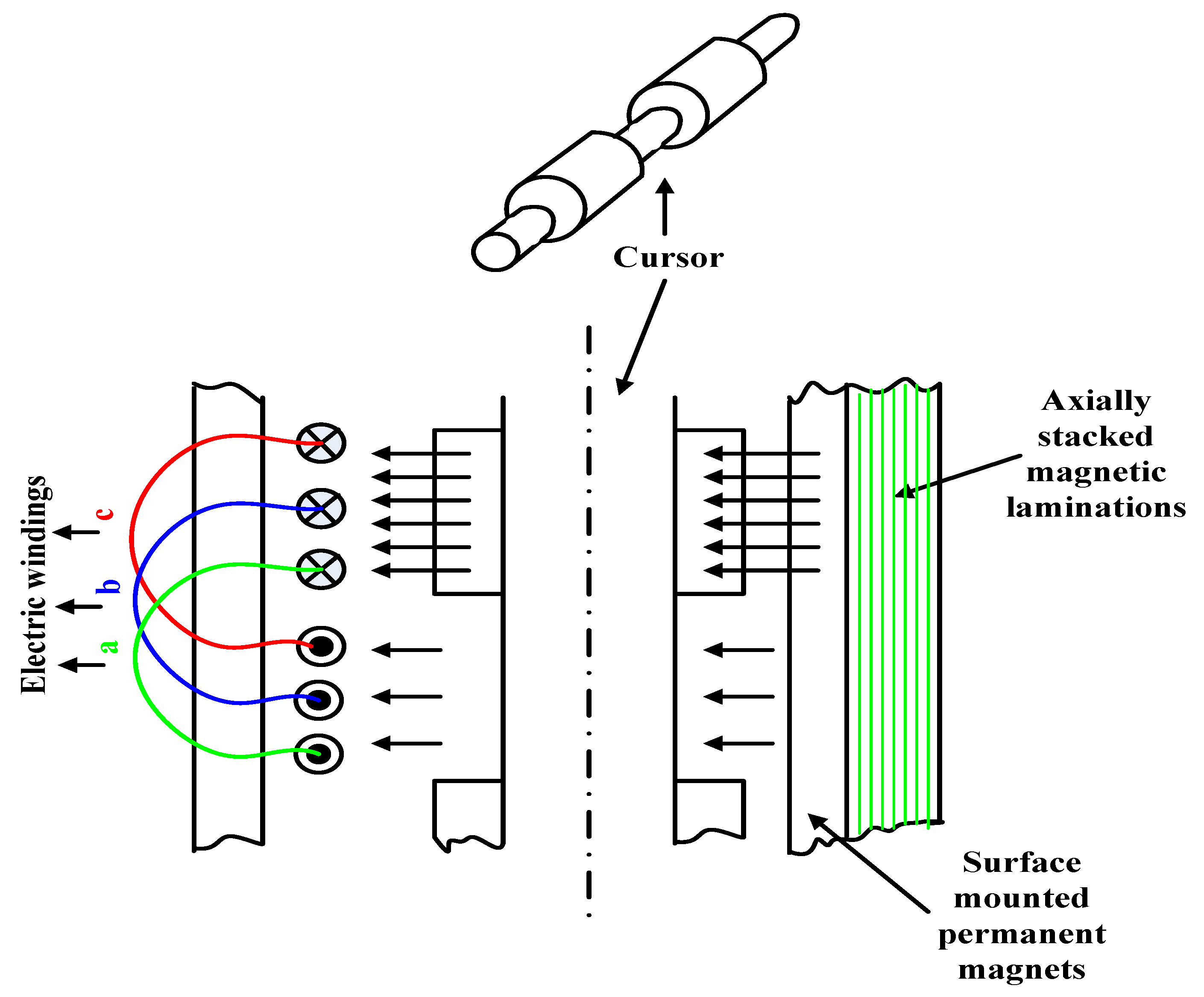
As shown in Figure 2, both the feeding coils and permanent magnets are set in the same section of the motor itself. The magnets are arranged so that the direction of the magnetization is always from the stator to the cursor so that the excitation circuit and the armature winding are placed on the same magnetic core; for this reason, the name homopolar is given to the motor. The flux lines of the permanent magnets in the outer-part are always perpendicular to the axis of the motor. Moreover, the external motor’s cover is advantageously constructed with axially stacked magnetic laminations in order to minimize iron losses.
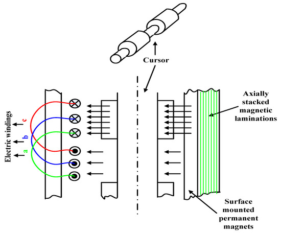
Figure 2.
Cross-section of the LT-H motor showing the interaction between permanent magnets and the motor’s windings.
The windings used in the LT-H motor are similar to those of rotary induction motors. As the magnets and windings are both set within the stator, the cursor is thoroughly passive, and thus it comes out from the stator without causing any related issues. It is worth mentioning that the LT-H motor can be constructed without permanent magnets, and in this case the motor will be very similar to the reluctance motor, with lower manufacturing costs; however, the thrust-force production will be reduced. The operation of the motor when loaded is described in the following paragraphs.
The motor windings are linked to the magnetic fields of the permanent magnet; at the same time, the currents flow in the windings, which finally results in generating a force because of the magnetic interaction. The value of the generated force is determined according to the position of the windings with respect to the cursor polar expansions; for example, maximum force is obtained when windings are in front of the cursor polar expansions, and vice versa.
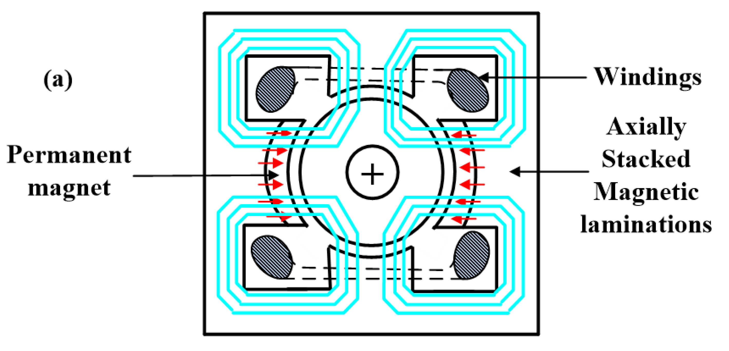
From Figure 2, it is noticed that the produced force is formulated of two contributions, relative to the two sides of the motor coil. As the direction of the magnetic flux density vector is the same, while the current directions on the two coils’ sides are opposite to each other, then the two forces’ contributions along the axial direction have opposite directions. However, due to the large flux density with respect to the cursor polar expansions, the output force will fulfill the movement task. When the cursor begins to move, the currents are synchronized with the cursor movement, in order to obtain a force with the same direction. Another cross-sectional view of the LT-H motor is also shown in Figure 3 that illustrates the positions of the motor coils and the distribution of the field lines.
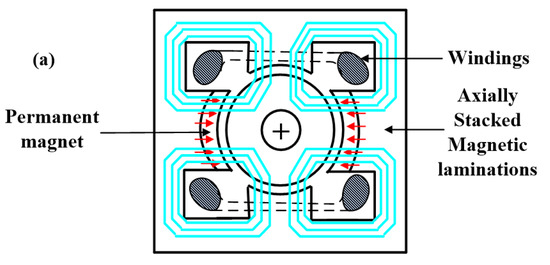
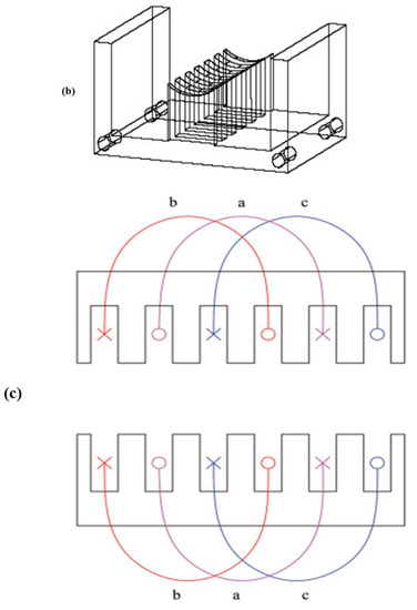
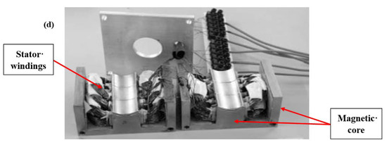
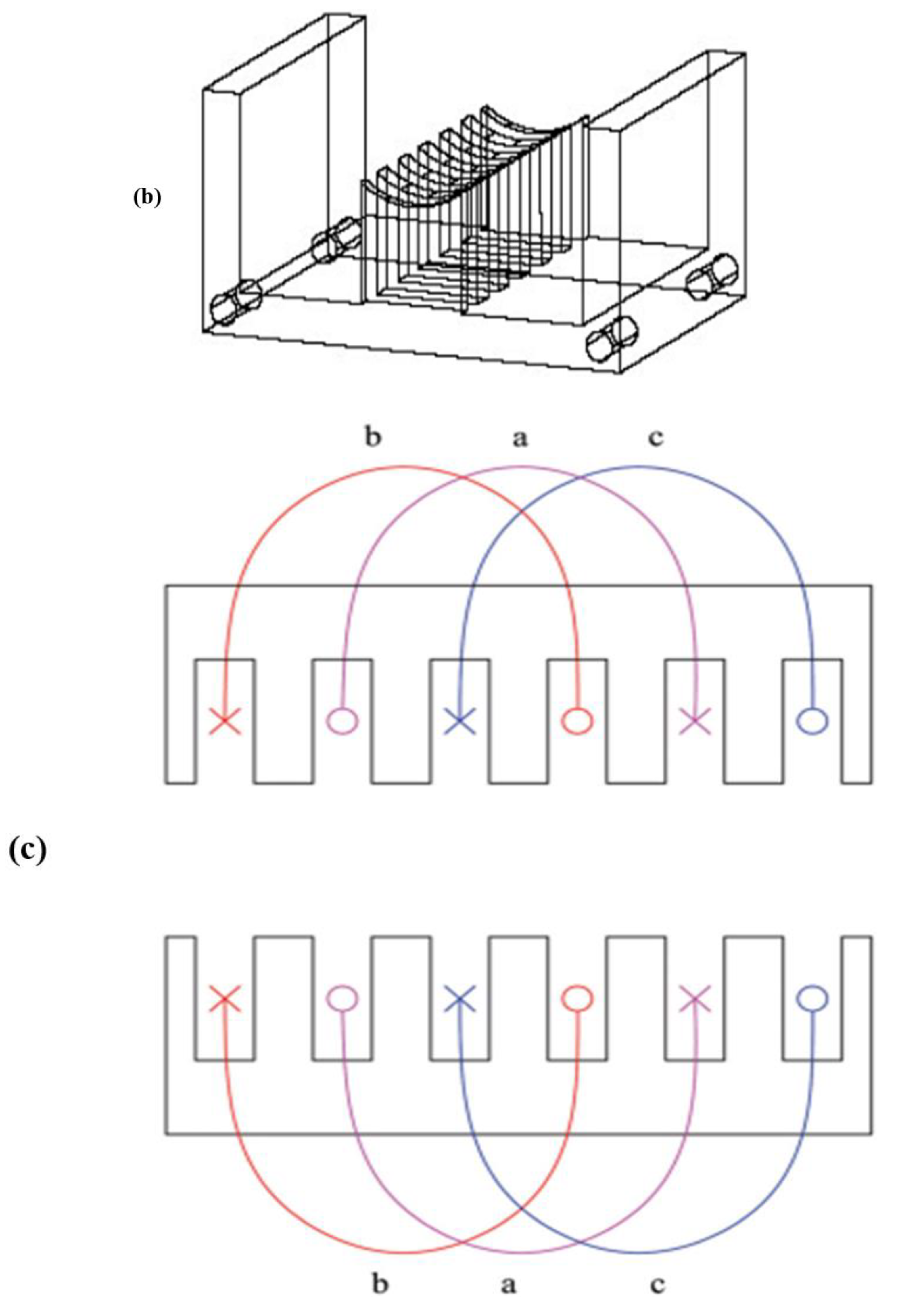
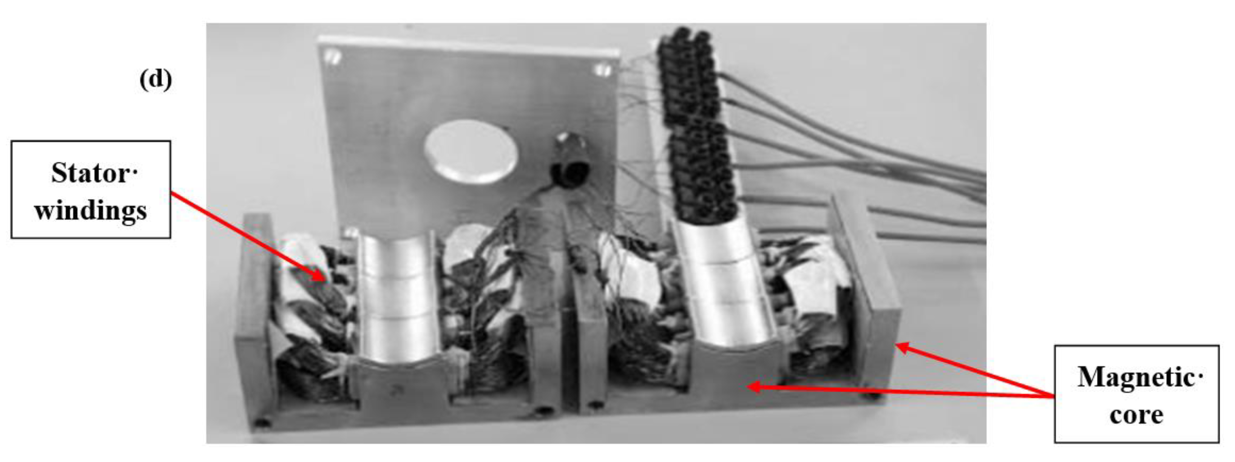
Figure 3.
(a) Cross-section of the LT-H motor showing winding positions and magnetic field lines; (b) 3D view of the magnetic core; (c) illustration of the stator windings; (d) general sectioned LT-H motor.
1.2. Mathematical Modeling
From an electrical point of view, the linear motor has equations very similar to those of the permanent magnet synchronous motor with anisotropic rotor. To describe the motor’s behavior, we can therefore consider the same general equations of the voltage balance:
where ua, ub, uc, ia, ib and ic represent the voltages and currents of the phases, and ψa, ψb and ψc are the fluxes, whereas R = 4.65 Ω represents the windings resistance.
Assuming that the magnetic circuit is not in saturation, the total magnetic flux linked by each phase can be calculated as the sum of two contributions: one term originates from the presence of permanent magnets, and one originates from the currents circulating in the phases.
In the absence of current in the phases, the flux is determined only by the permanent magnets. From the theory of homopolar synchronous motors with permanent magnets (the reference coordinate in the linear motor is given by the direction of motion along the z axis (along the cursor), not by the electrical angle ; however, the formulas are the same if we set the equality , where is the pole-pitch, is the cursor displacement and is the angle between the axis of phase ‘a’ and that of the field produced by the permanent magnets), then we obtain:
where ,and .
The self and mutual inductances of the motor’s windings are expressed by (3) and (4):
where , , , and .
All these expressions can be written in a more compact form using vector notations as follows:
with and .
The resistances, inductances and back-emf matrices are expressed by:
where .
The flux matrix is expressed by:
where θme is the electrical angle between the axes of phase ‘a’ and that of the field produced by the permanent magnets.
1.2.1. Modeling in d-q Reference Frame
Calculation of Inductance Matrix
The inductance matrix in the dq0 reference (Ldq0) is obtained from the Labc matrix as follows:
The transformation matrix from the system abc to dq0 can be expressed by:
where θg indicates the position of the system d-q with respect to the stationary α-β system.
Then, the inverse transformation of (9) can be defined by:
Considering the inductance matrix Labc in (6), and by substituting from (3) and (4), the following expression is obtained:
Via applying the transformation in (8) on (11), the Ldq0 matrix is obtained as follows:
To synchronize the motor with the reference system dq0 (2θg = θme), the inductance matrix is further simplified by:
Calculation of Flux Matrix
Similar to what was done for the Ldq0 matrix, the flux matrix can be obtained via utilizing (8), (9) and (10) as follows:
The motor’s model can be synchronized with the reference system dq0 via putting (2θg = θme), and putting , then the flux matrix is further simplified by:
Considering that the resistance matrix R remains unchanged, we can write the system’s equations in the synchronous frame by:
where is the cursor displacement variation (velocity), p = 1 is the pole pairs and , , and . All motor data are also typed in Table A1 in the Appendix A.
1.3. Operation Regions for the LT-H Motor
The region of operation for the linear motor is set by the current and voltage limits imposed at the design stage (Un = 80 V, In = 5 A), which must be considered to ensure the correct operation of the drive.
To determine these limits, the motor’s equations at full-speed operation () are then considered, leaving out its behavior during transients, where higher limits can be allowed for limited times.
where f refers to the developed force.
The current and voltage limits can be expressed by:
Substituting from (17) and (18) in (21), it results in:
Then:
The relation (23) represents an ellipse centered at the following coordinate points:
Using (24), the current limits and the related iso force (f) curves can be correctly obtained.
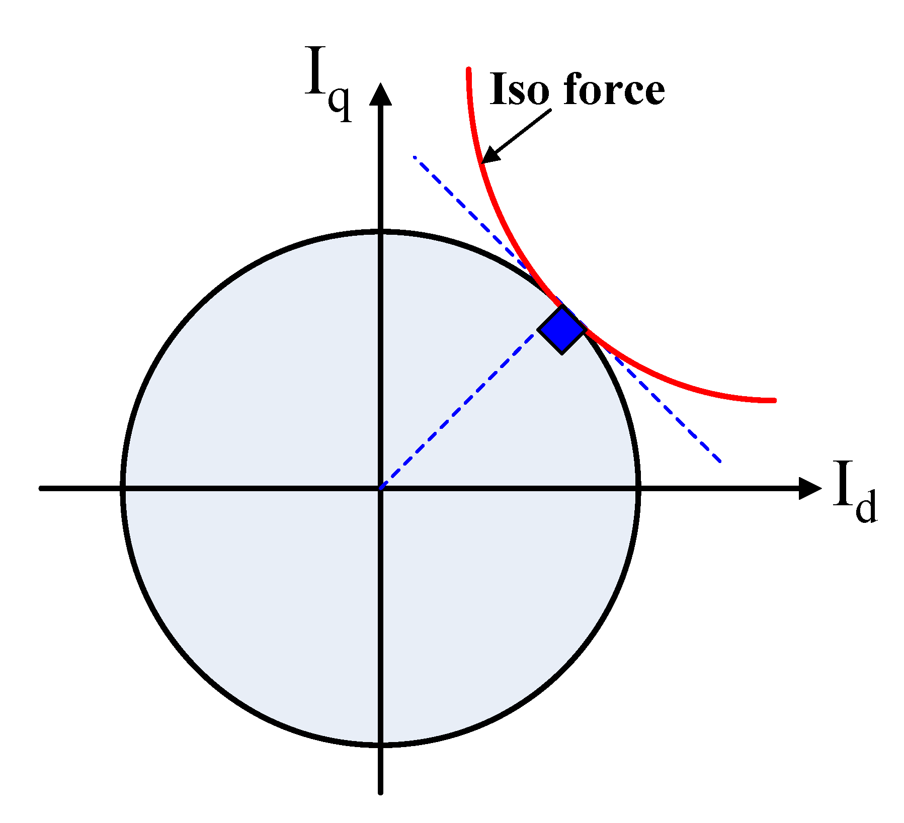
Expecting to operate the motor in the area with constant maximum force, it becomes interesting to analyze the equation that identifies the operation of the motor with the maximum force per current (MFPC) ratio, represented graphically, as the speed varies, by the set of points at which the current curve and the iso-force curve result in the same tangent. This calculation can be simplified by considering that the radius of the circumference passing through the tangent point must be perpendicular to the tangent line of the iso-force curve at the same point, as indicated in Figure 4.
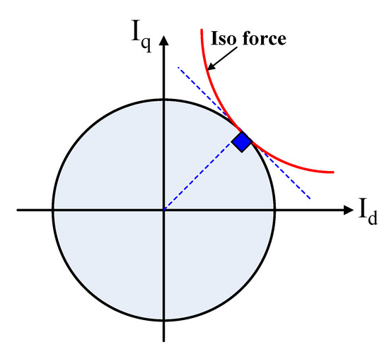
Figure 4.
Illustration of the tangent point between the iso force and current circumference.
From Figure 4, the angular coefficient of the radius can be calculated by:
From (19), the current is calculated by:
Taking the derivation of (26) with respect to id, the angular coefficient of the tangent line to the iso force curve is expressed by:
To maintain the perpendicularity between the d-q current components, it is necessary that:
Then, from (25) and (28), it results in:
By substituting from (19) into (29), then the relationship between the q and d components of the current is expressed by:
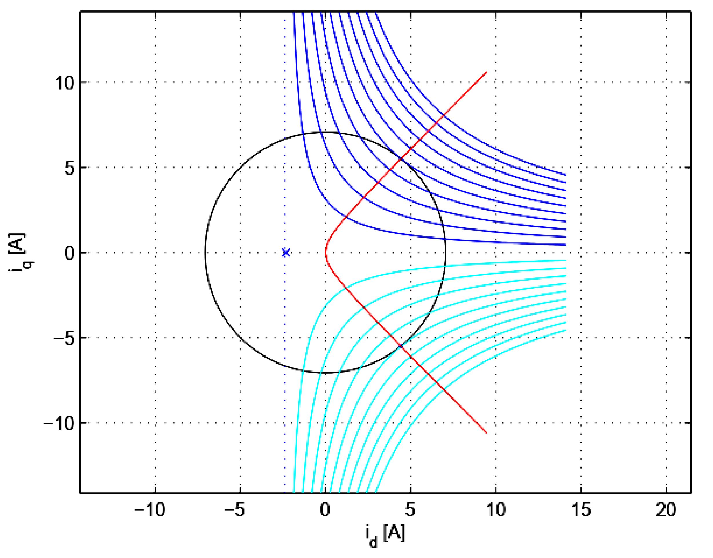
Through plotting (30) and also adding the iso-force curves to the plot, the maximum force per ampere curve (red line) can be obtained as illustrated in Figure 5.

Figure 5.
Operating regions with max force per current curve (red).
Once the maximum force-current operating curve is identified, the maximum values of id and iq currents can be obtained as follows:
Using these values, and through (19) and (22), the calculation of the base displacement zbase and nominal force is performed as follows:
where
The nominal force can be calculated by:
2. Control-System Design
The proposed control system for the LT-H motor consists of two main loops: the current (id, iq) control loop and the velocity control loop.
2.1. Design of the Current Control Loops
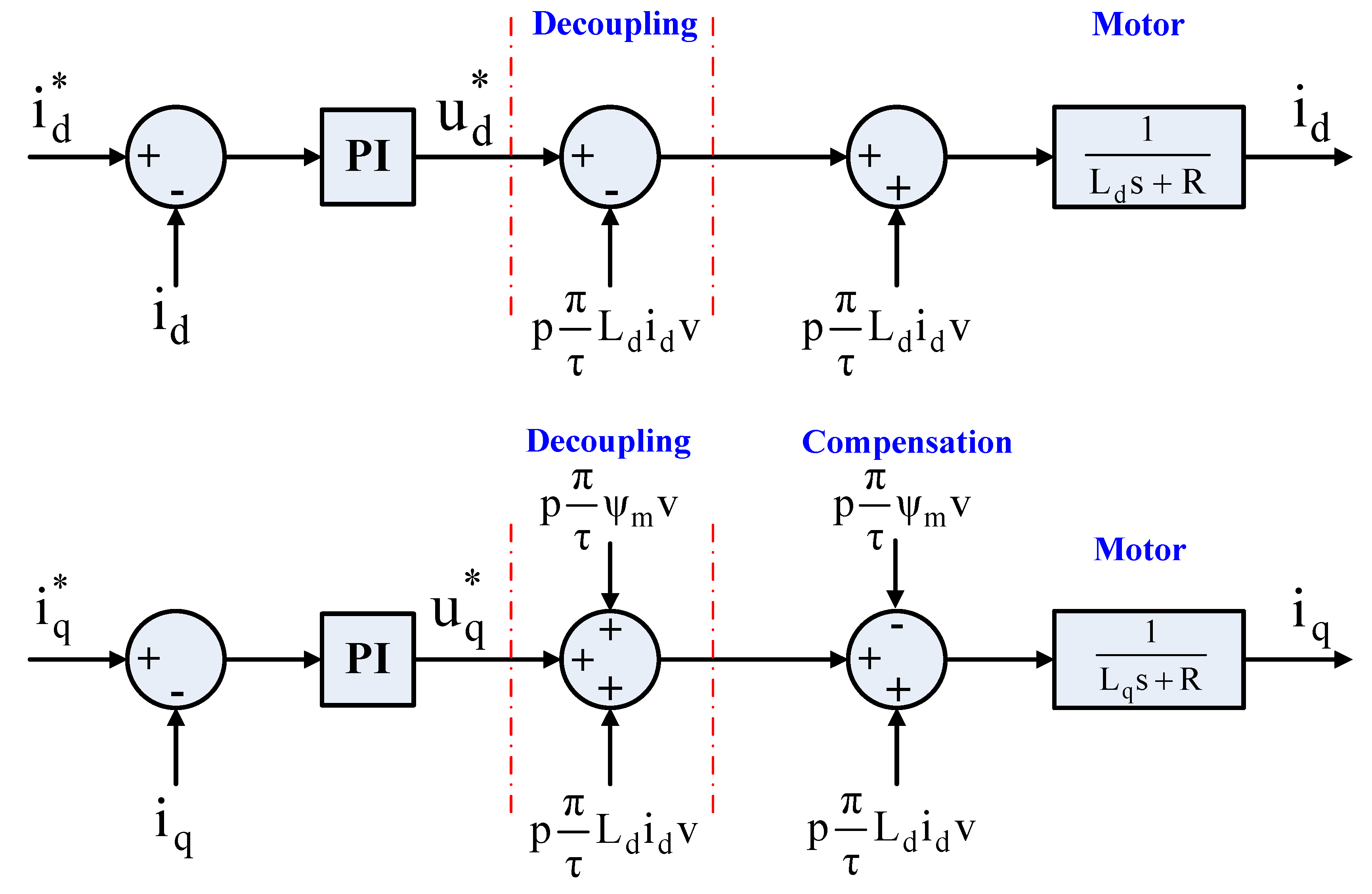
Two regulators were developed, one for the current iq and one for the id that guaranteed a bandwidth of 500 Hz for both. Before analyzing the loops, it was decided to decouple the two current branches through eliminating the mutual coupling between the d and q components, adding to the output of the regulators a contribution equal and opposite to that present inside the motor model, as shown in Figure 6.

Figure 6.
Decoupling of d and q current components.
From Figure 6, the open-loop transfer function of id current including the regulator can be expressed by:
where .
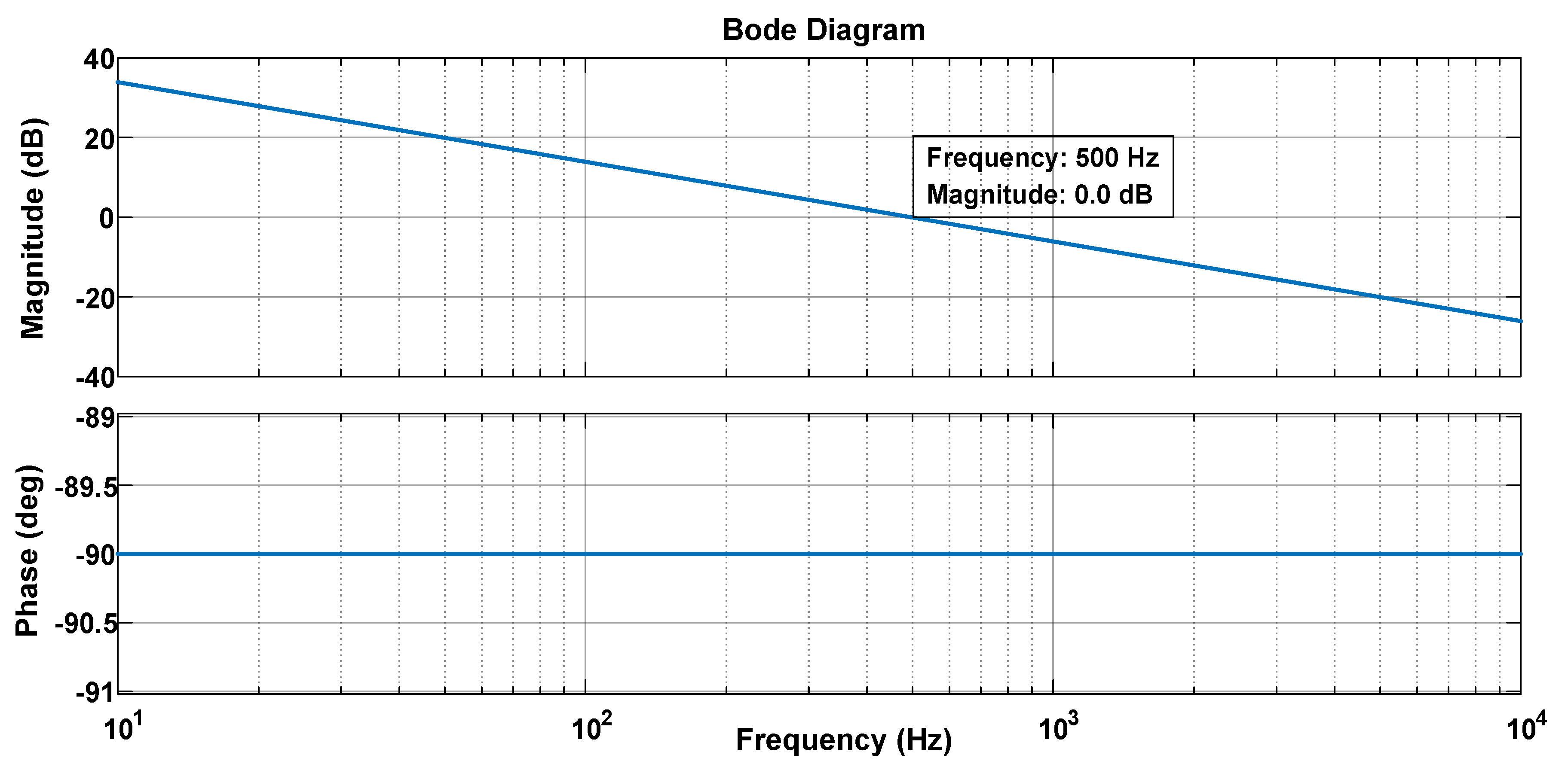
Assuming that the zero of the PI regulator cancels the dominant pole of the transfer function that represents the motor dynamics with a crossover frequency equal to , and by imposing and , the following is obtained:
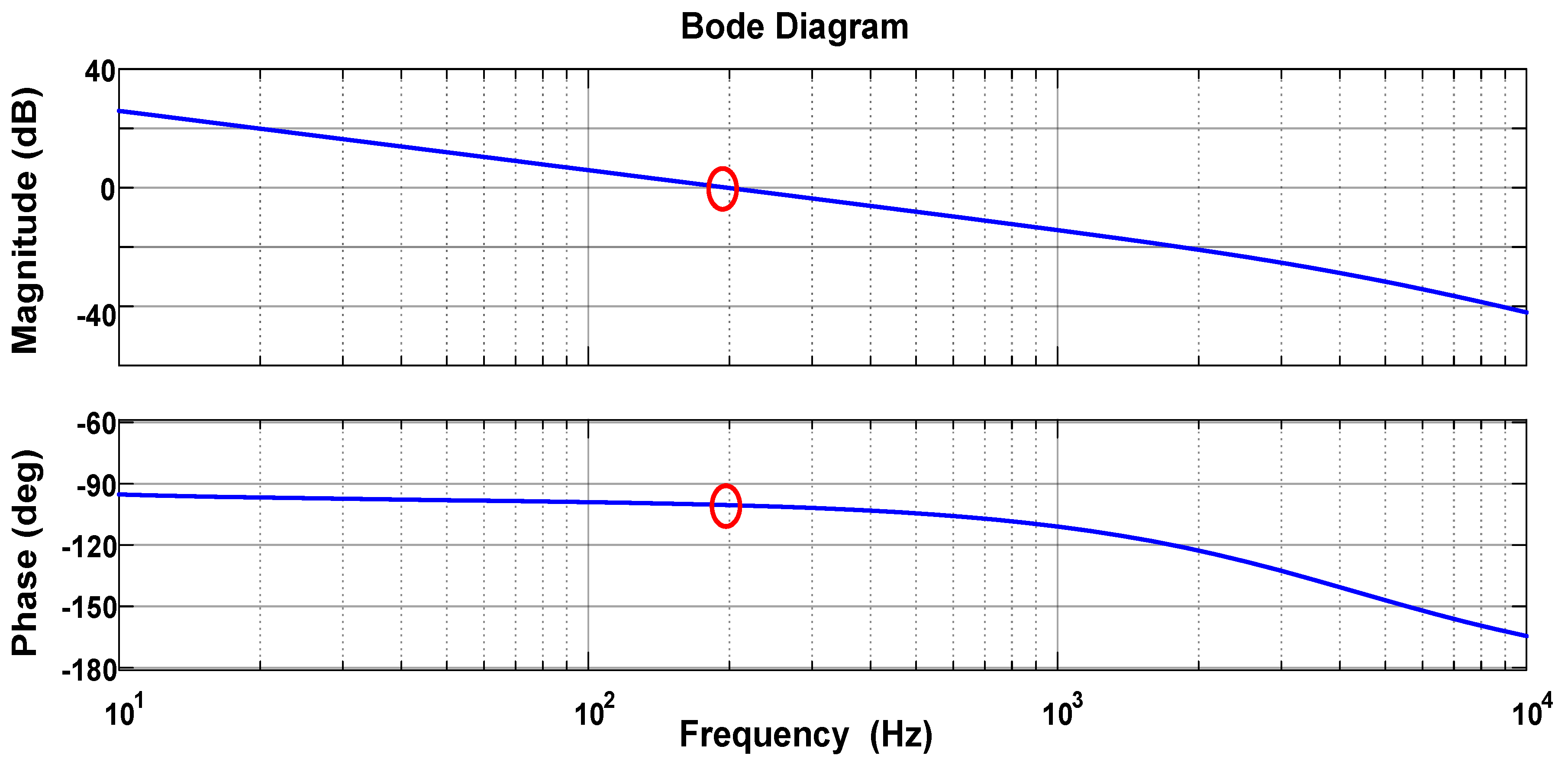
Figure 7 shows the bode plot of the transfer function; from which it can be observed that the phase margin is approximately equal to 90° degrees, which reveals the validity of the design procedure.
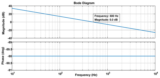
Figure 7.
Bode plot for the transfer function of the d-axis current loop.
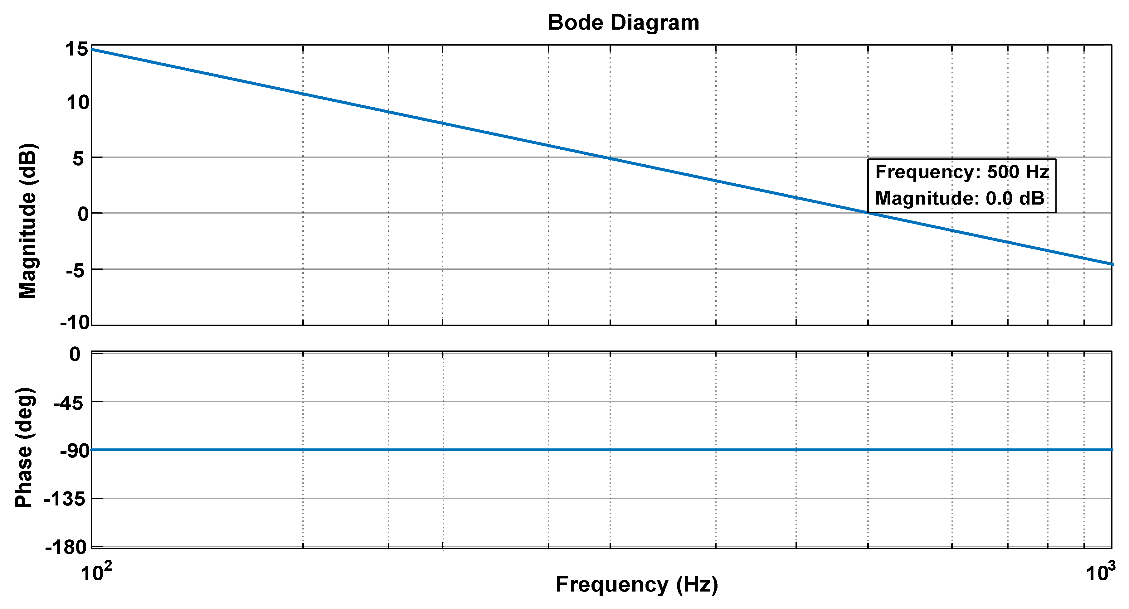
As illustrated in Figure 6, after compensating for the counter-electromotive force, the block diagram of the q-axis current loop appears to be similar to that of the direct axis. Then, similar to what was done for the direct axis by assuming that the zero of the regulator cancels the dominant pole of the function with crossing frequency of and , the following parameters are obtained:
Then, by plotting the bode plot of the transfer function for the iq current loop as shown in Figure 8, it is revealed that a phase margin of 90° is obtained, which confirms the validity of the designed regulator.
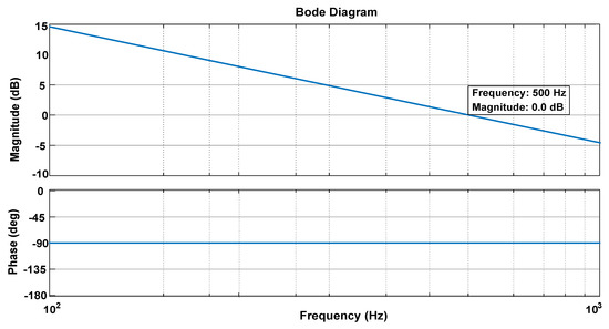
Figure 8.
Bode plot for the transfer function of the q-axis current loop.
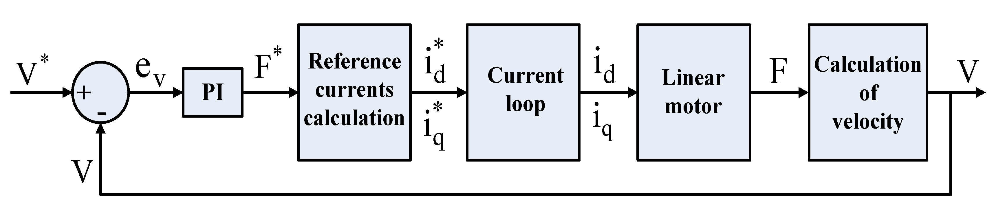
2.2. Design of the Velocity Control Loop
The scheme used for designing the parameters of the velocity regulator is shown in Figure 9. In the following subsections, the description of each block in the scheme will be provided, and some linearizations are introduced to size the velocity regulator.
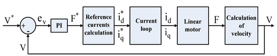
Figure 9.
Velocity control loop.
2.2.1. Current Loop Transfer Function
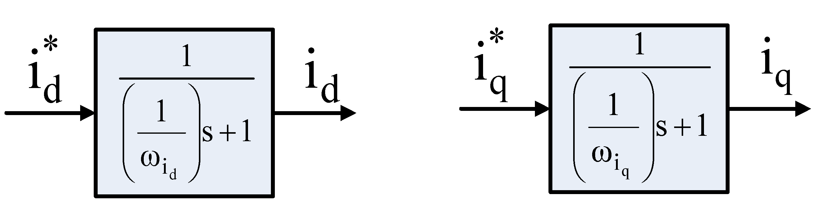
Some simplifications were made in the study of the velocity loop; the first was to approximate the transfer functions of the current loops to a first-order function with a crossing frequency set to 500 Hz.
This approximation is well justified from the theoretical point of view: in fact, considering the generic transfer function depending on whether the value of the product G(s)*H(s) is greater than 1, resulting in a good approximation in the bandwidth, or lower than 1, that is, for frequencies greater than the crossing one, which results in and , respectively. With this choice, the current loop blocks are the ones shown in Figure 10:
where and . Meanwhile, are the crossover frequencies.
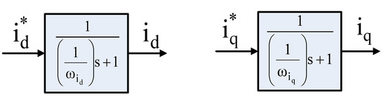
Figure 10.
Current loops.
2.2.2. Calculation of Reference Currents
Numerical Solution
The reference currents are calculated based on the value of the force required from the motor. This can be performed through analyzing the relationship between the force and the q-axis current component. Using (19) and (30), and after derivation, this results in:
where , , , , , , , , , .
The complexity of the obtained solution does not allow the numerical calculation of the velocity loop’s transfer function, since it foresees divisions 0 on 0 that the calculation program is not able to manage; it was therefore necessary to switch to an alternative solution.
Solution Through Linearization [iq = iq(f)]
The need to make a simplification in (39) has led to approximating the id curve to be a straight line; thus:
where .
Replacing (40) into (19), it results in:
where the + sign is considered when f > 0, and the − sign when f < 0.
2.2.3. Mass (m) and Friction (F) Parameters
The velocity calculation block is constructed directly through the linearization of the mechanical load equation defined by:
where
- m = 0.996 Kg represents the mass of the slider;
- F = 0.4980 N is the dynamic friction component; and
- fl is the load force.
Finally, the load force during the design of the velocity controller was treated as a disturbance, and therefore considered null in this analysis.
2.2.4. Design of Velocity Regulator
By reconsidering the block diagram in Figure 9, it is now possible to pass to the determination of the parameters of the velocity regulator and analyzing the velocity-loop transfer function via combining all blocks’ functions as follows:
where .
By assuming that the zero of the regulator cancels the denominator’s pole given by the term , with a bandwidth frequency of ( rad/s), with and , then the following gains are obtained:
Thus, the designed regulator allows a bandwidth frequency of 200 Hz with a phase margin of about 68°, as shown in Figure 11.
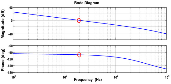
Figure 11.
Bode plot for the transfer function of the velocity loop.
3. Proposed Estimator
In order to enhance the control system’s robustness, an estimator is designed to observe the motor’s velocity and stator resistance in parallel. The design procedure can be described in a systematic way as follows:
From (16), the stator voltage d-q components can be reformulated in terms of the estimated velocity in the synchronous rotor frame by:
From (46) and (47), the rotor’s back-emf can be evaluated by:
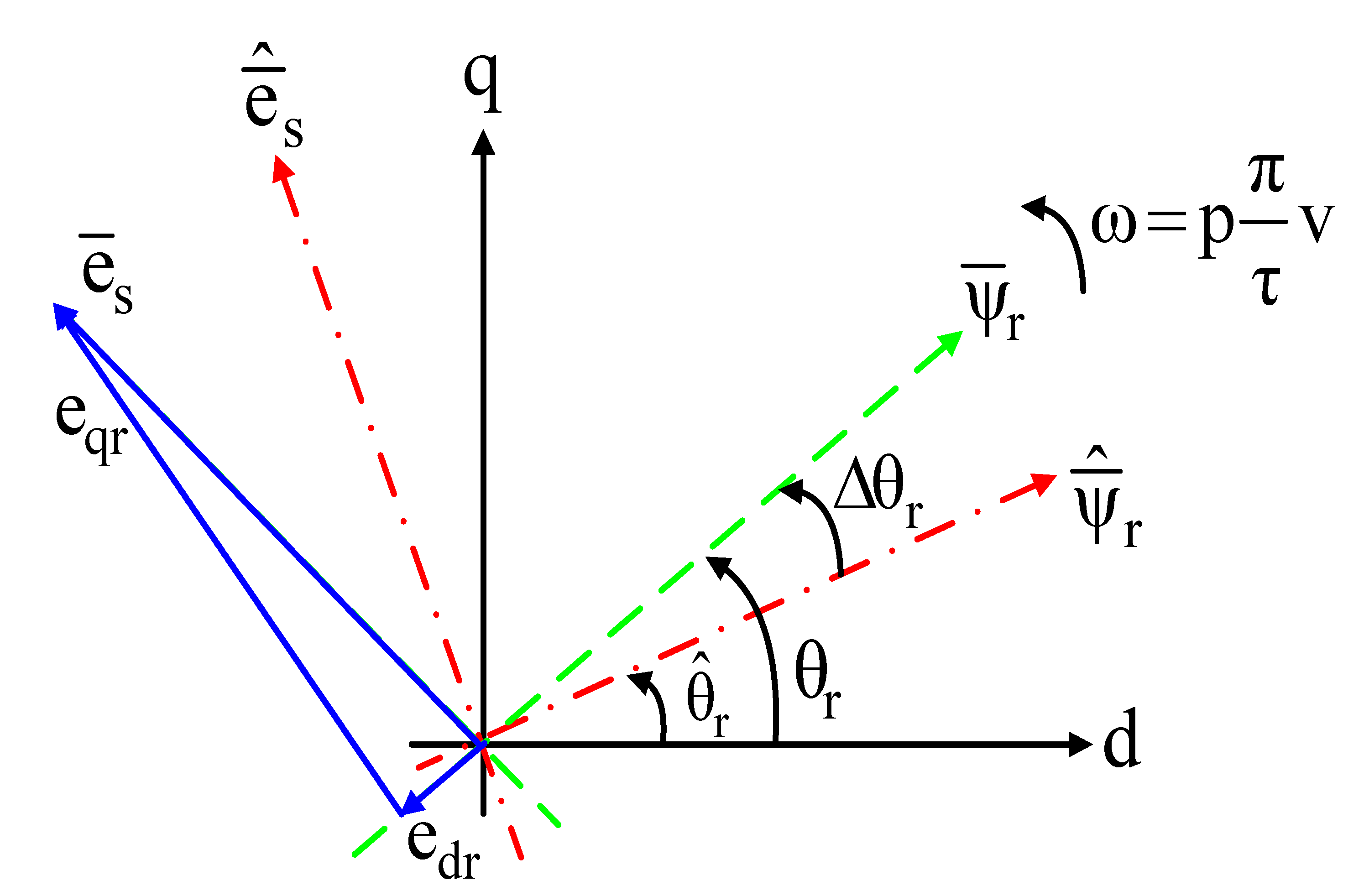
The imprecise flux orientation causes an error in the mutual induced back-emf, as shown in Figure 12.
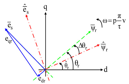
Figure 12.
Misalignment between actual and estimated rotor flux vectors.
From Figure 12, it is noted that there is an error between the actual and estimated rotor flux vectors. It is also noted that the back emfs and are perpendicular to the actual and estimated flux vectors, respectively.
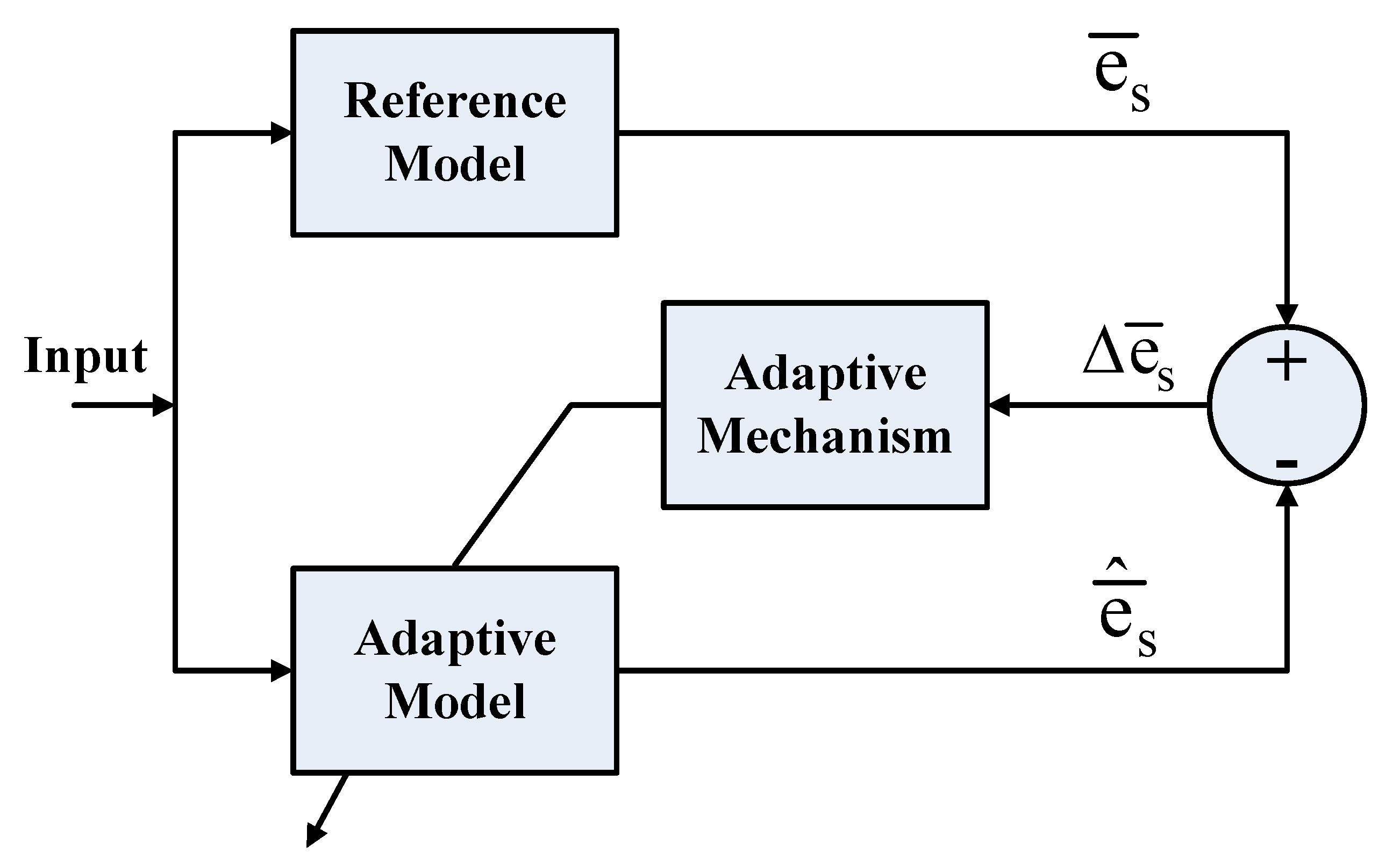
As the velocity and resistance values are extracted from the error between two models: reference model which utilizes the real back-emf () and an adaptive model which provides the estimated back-emf () as shown in Figure 13.

Figure 13.
Configuration of the back-emf-based adaptive estimator.
To achieve a correct estimation, the real back-emf must be precisely evaluated. However, the real back-emf cannot be directly evaluated, as the rotor position is also unknown during the sensorless operation. As a solution to this problem, the estimated rotor flux axis is considered as a reference to obtain the actual back-emf . This is illustrated in Figure 12, as the vector is obtained after the vector summation of the rotor emfs ( and ), then:
The actual back-emf in (50) can be obtained via differentiating the rotor flux vector as follows:
Now, if the estimated and actual fluxes are appropriately oriented (), then the actual rotor flux can be evaluated by:
Consequently, the observed back-emf can be calculated by:
The difference between the actual emf and estimated emf is the resultant error signal which must be minimized in order to make the actual and estimated fluxes identical.
From (49), (53) and (54), the error signal that will be utilized to estimate the motor velocity can be expressed by:
The calculated error in (55) is then applied to an anti-windup PI regulator, which finally provides the estimated velocity at its output.
From (55), it can be noticed that the accurate acknowledgement of R is a vital requirement for the correct estimation, especially at low operating frequencies.
The resistance R can be estimated through regulating the deviation between the actual and estimated airgap powers ( and ). The observed power can be calculated in terms of the estimated velocity and observed rotor flux by:
On the other hand, the actual power can be evaluated through subtracting the power loss in R from the input power as follows:
Thus, if the correct estimation is ensured, the two powers should have the same value, otherwise a deviation appears in case of the resistance variation.
The power deviation can be expressed by:
where and are the stator and rotor back-emfs. Then, by replacing from (53) into (54), it gives:
It is noted from (59) that the second term of error signal is almost the same as the term used to estimate the velocity, and to avoid any conflict, the error signal is simplified to consist only of the term multiplied by the sign of the estimated velocity as follows:
After that, the stator resistance variation can be obtained through feeding the error signal to a PI regulator, and finally the estimated resistance can be evaluated as follows:
where is the sampling time.
4. Overall System Structure
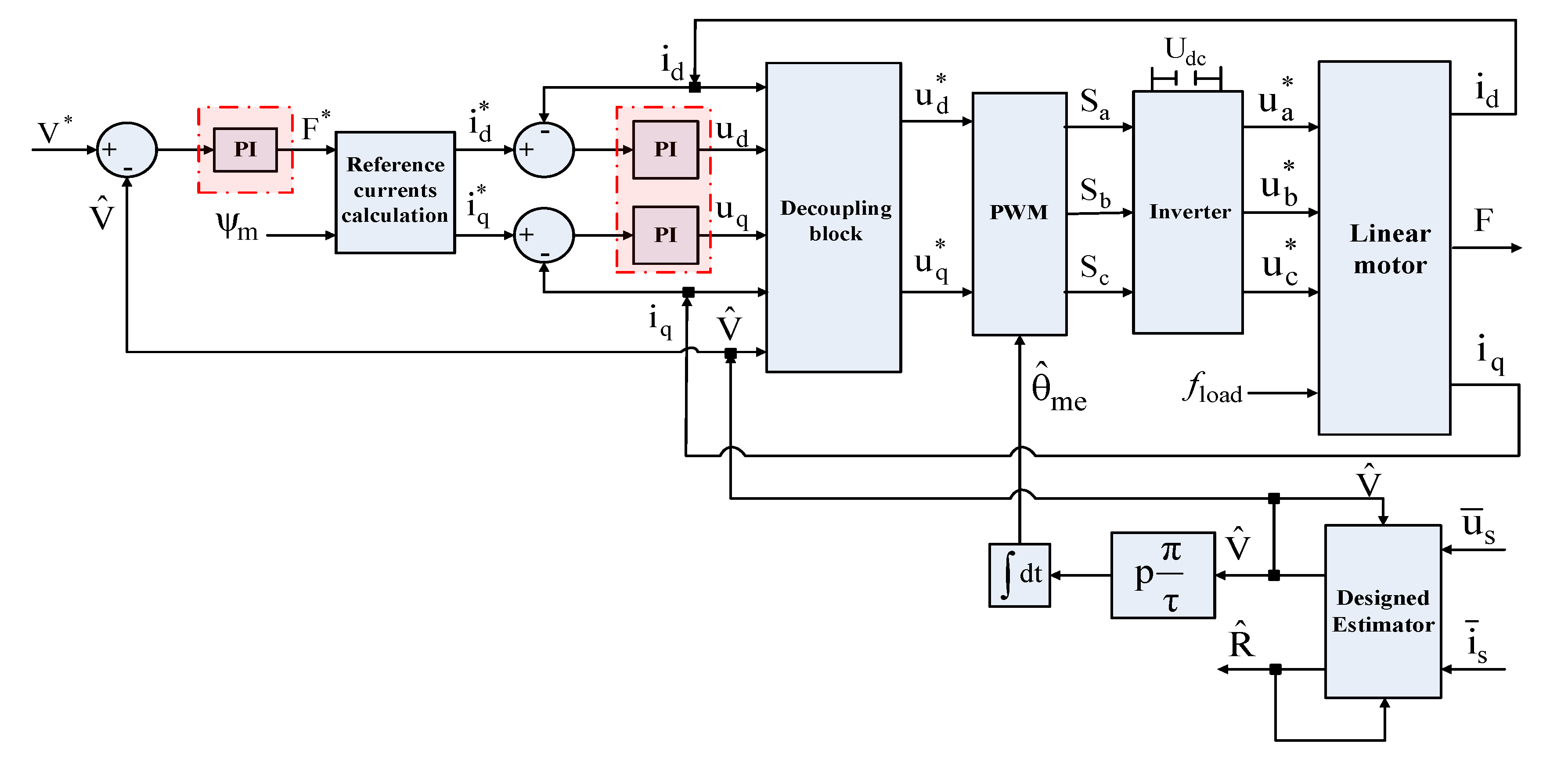
Figure 14 illustrates the complete layout for the designed control system for the LT-H motor type. The main control units are the designed velocity and d-q current PI regulators. The designed PI velocity regulator receives the velocity deviation () and provides the reference force command , which is used besides the flux value to calculate the reference d-q currents (,). The velocity is estimated using the designed observer described in Section 4. After that, the reference currents are compared with the actual motor currents, and the resultant errors are fed to the designed PI current regulators to provide the reference voltage components, which are then fed to the decoupling stage explained in Section 3 and shown in Figure 6 in order to finally provide the reference voltages and . The decoupled reference voltages are finally applied to the stator terminals through a PWM technique, which is combined with a filter to smooth the voltages applied to the motor.
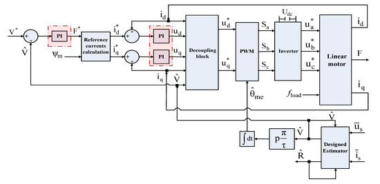
Figure 14.
Complete system layout for the designed controller.
5. Results and Discussion
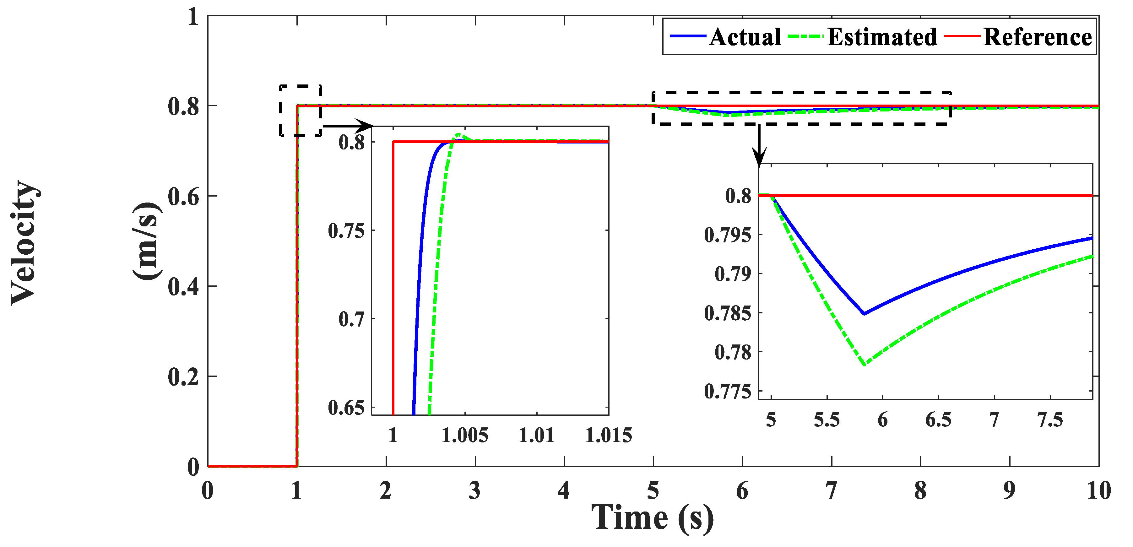
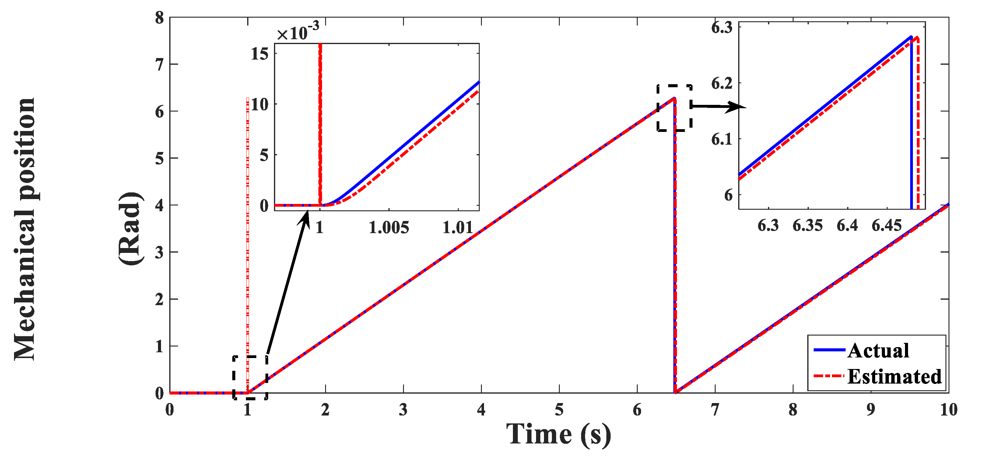
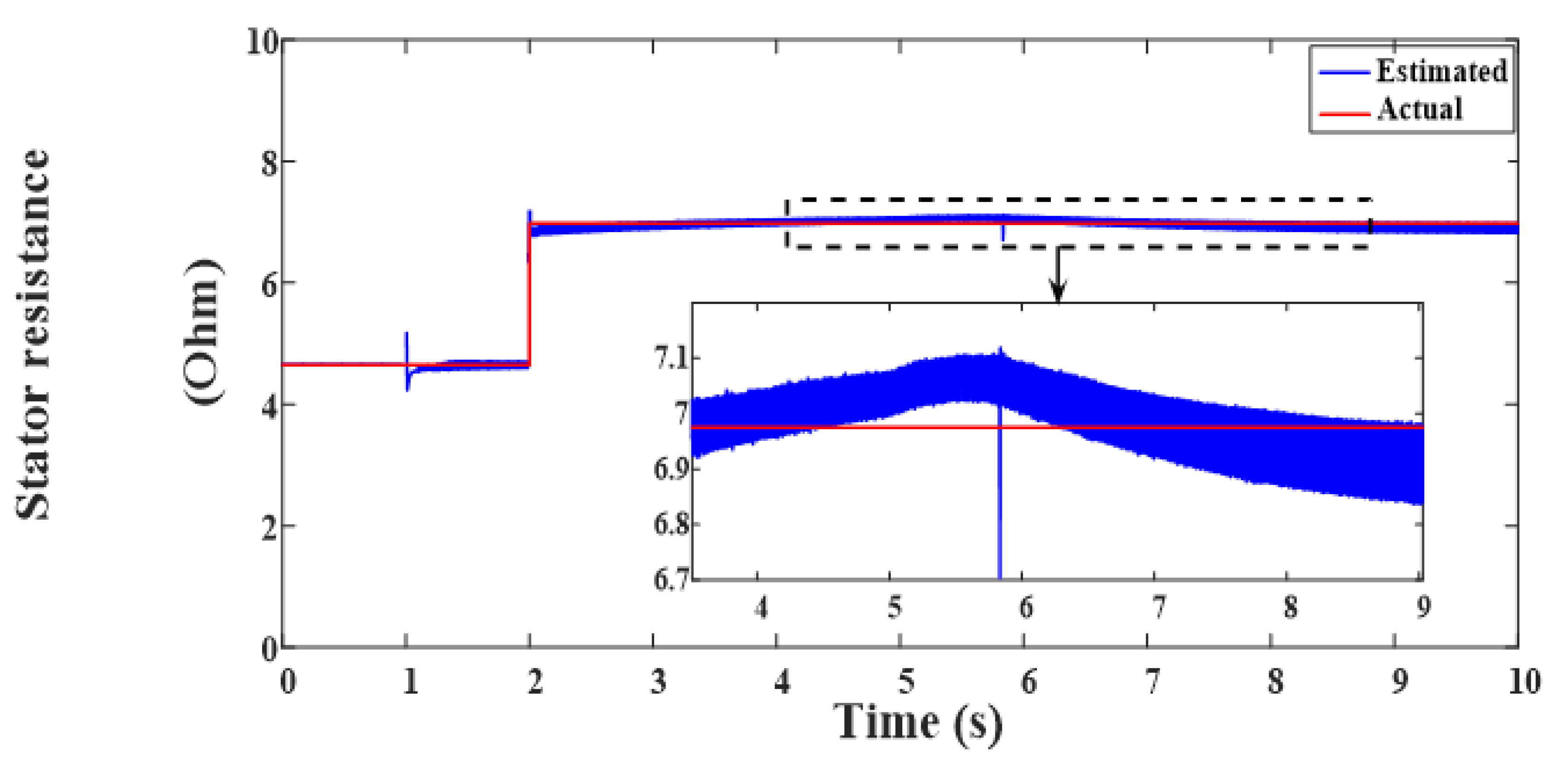
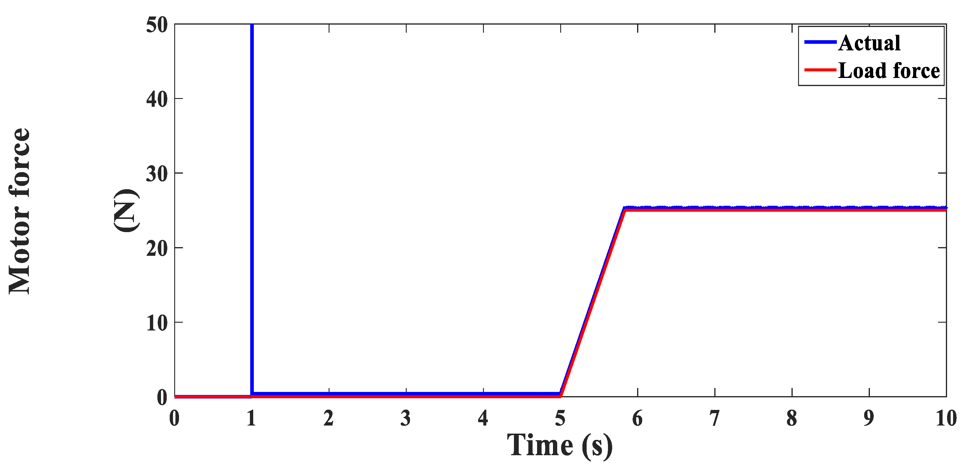
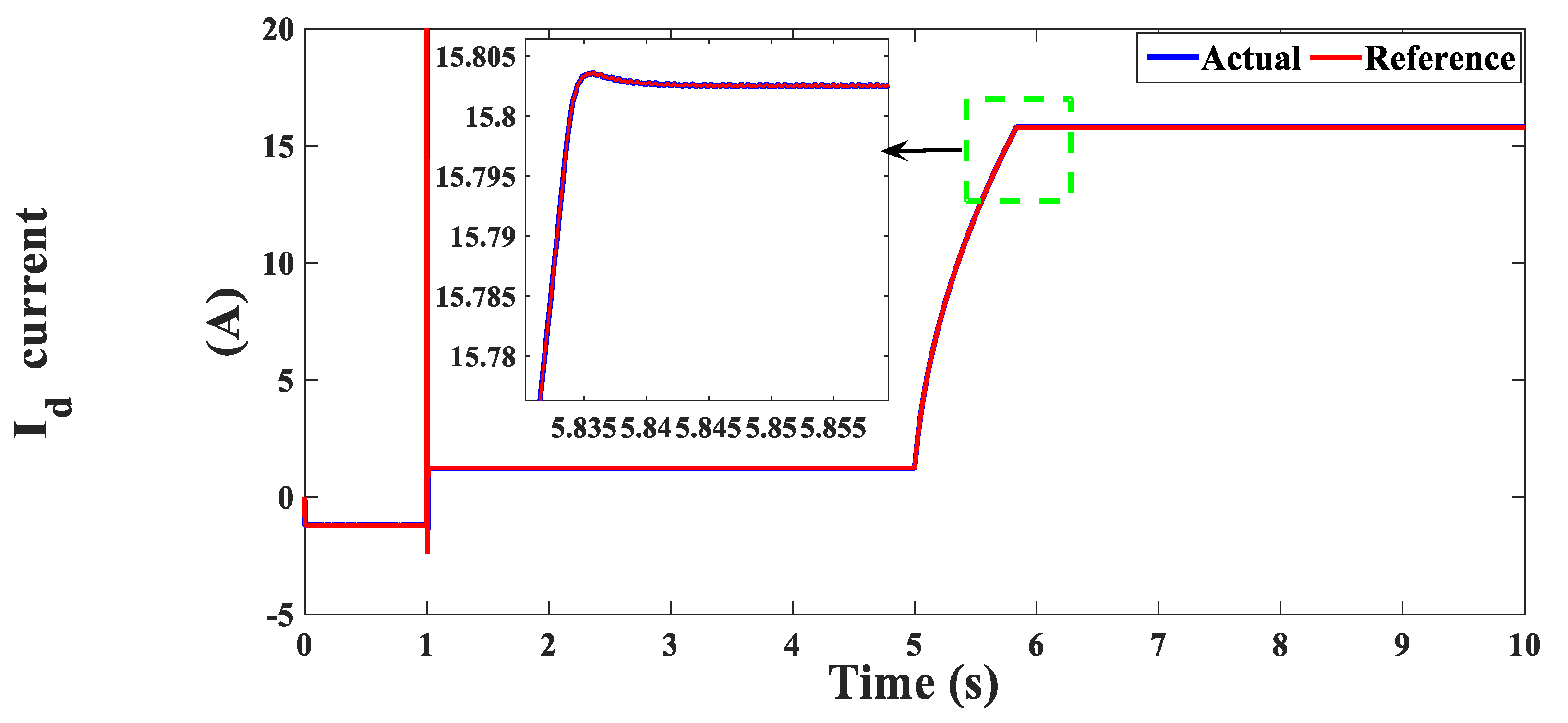
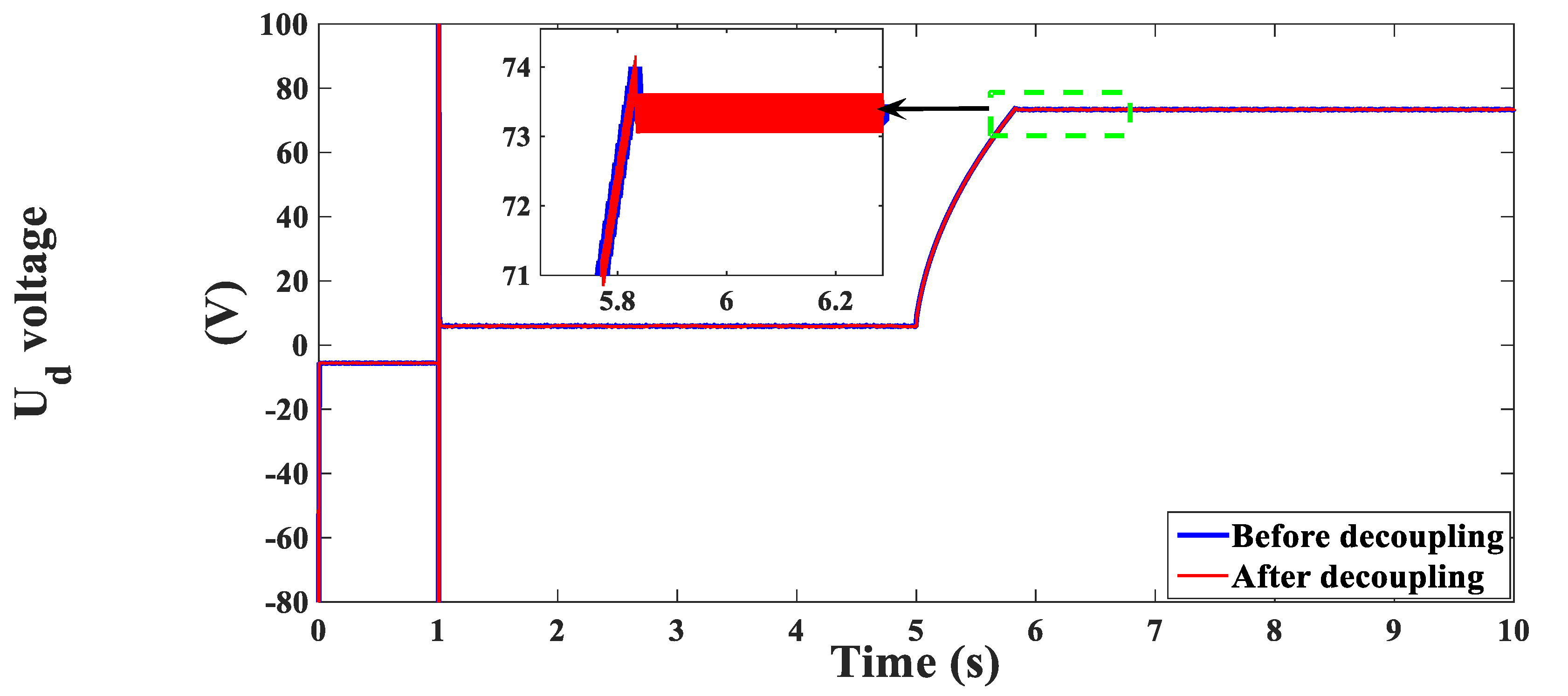
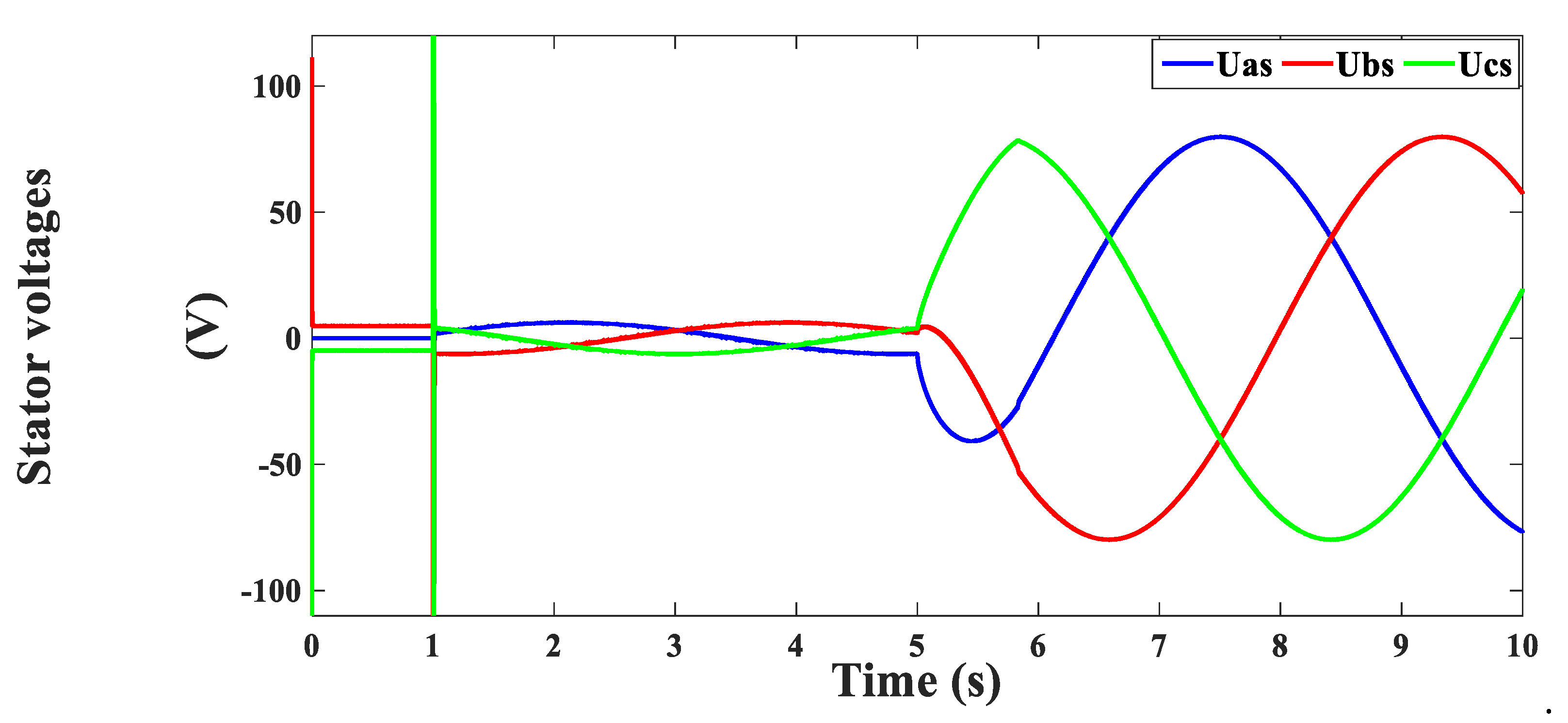
In order to test the effectivity of the designed sensorless control scheme, the tests were carried out in different manners using MATLAB/Simulink. The first test was performed by applying a reference velocity signal of 0.8 m/s at time t = 1 s, while a slope rising load force of 25 N was applied at time t = 5 s. The obtained results approved the validity of the controller in achieving a very good tracking of the reference velocity and applied load force. Figure 15 shows that the actual and estimated velocity signals definitely were following the reference signal. The estimated velocity also exhibited a very good dynamic with respect to the actual signal. Figure 16 reveals the actual and estimated rotor positions, which reconfirmed the observer’s validness. A resistance change of 1.5 times the actual value was made at time t = 2 s. Figure 17 shows the actual and estimated stator resistance, which clarified that the estimator was able to track the resistance change, which contributed effectively in enhancing the robustness. Figure 18 illustrates that the actual force was tracking the applied force with high precision. Figure 19 and Figure 20 show the actual and reference values of d-q stator currents. The currents were clearly following their references thanks to the appropriate design of the regulators. Figure 21 and Figure 22 show the un-decoupled and decoupled d-q voltage components, while Figure 23 presents the three-phase stator voltages. Finally, Figure 24 shows that a perfect decoupling was achieved between the d-q flux components thanks to the designed controller.

Figure 15.
Motor velocity (m/s).
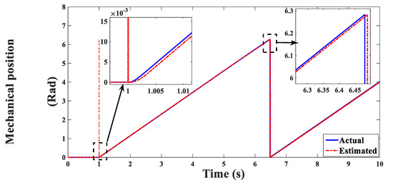
Figure 16.
Mechanical position (Rad).

Figure 17.
Resistance variation (Ω).

Figure 18.
Motor force (N).
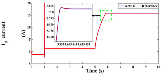
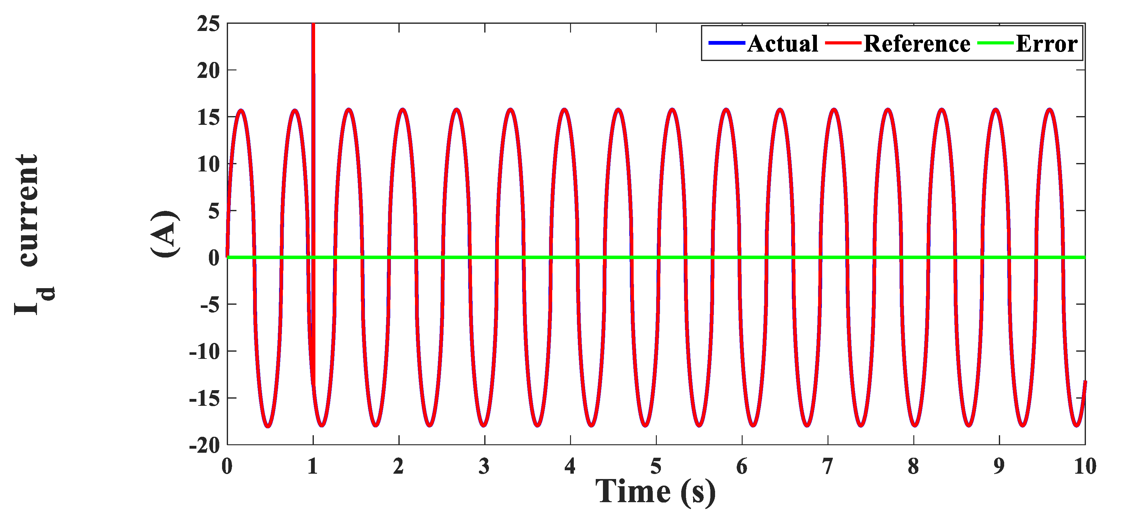
Figure 19.
The d-component of the stator current (A).
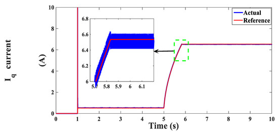
Figure 20.
The q-component of the stator current (A).
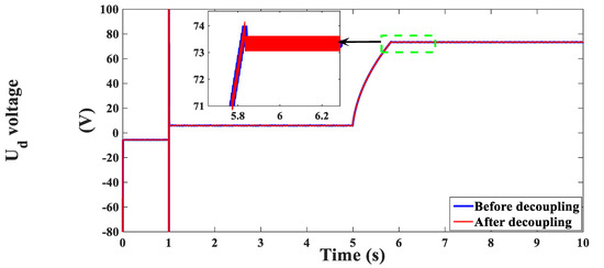
Figure 21.
The d-component of the stator voltage (V).
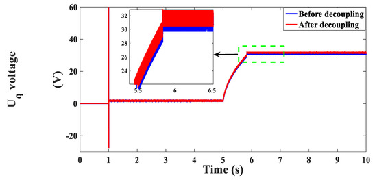
Figure 22.
The q-component of the stator voltage (V).
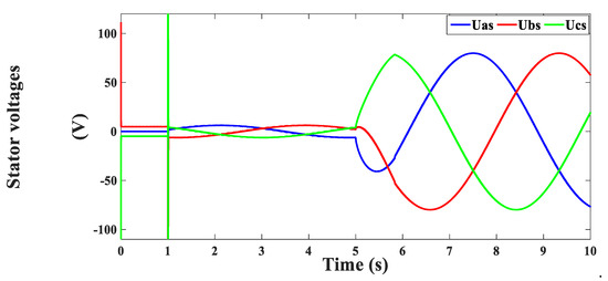
Figure 23.
Stator voltages (V).
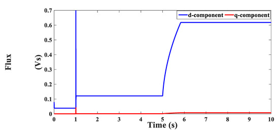
Figure 24.
Flux components (Vs).
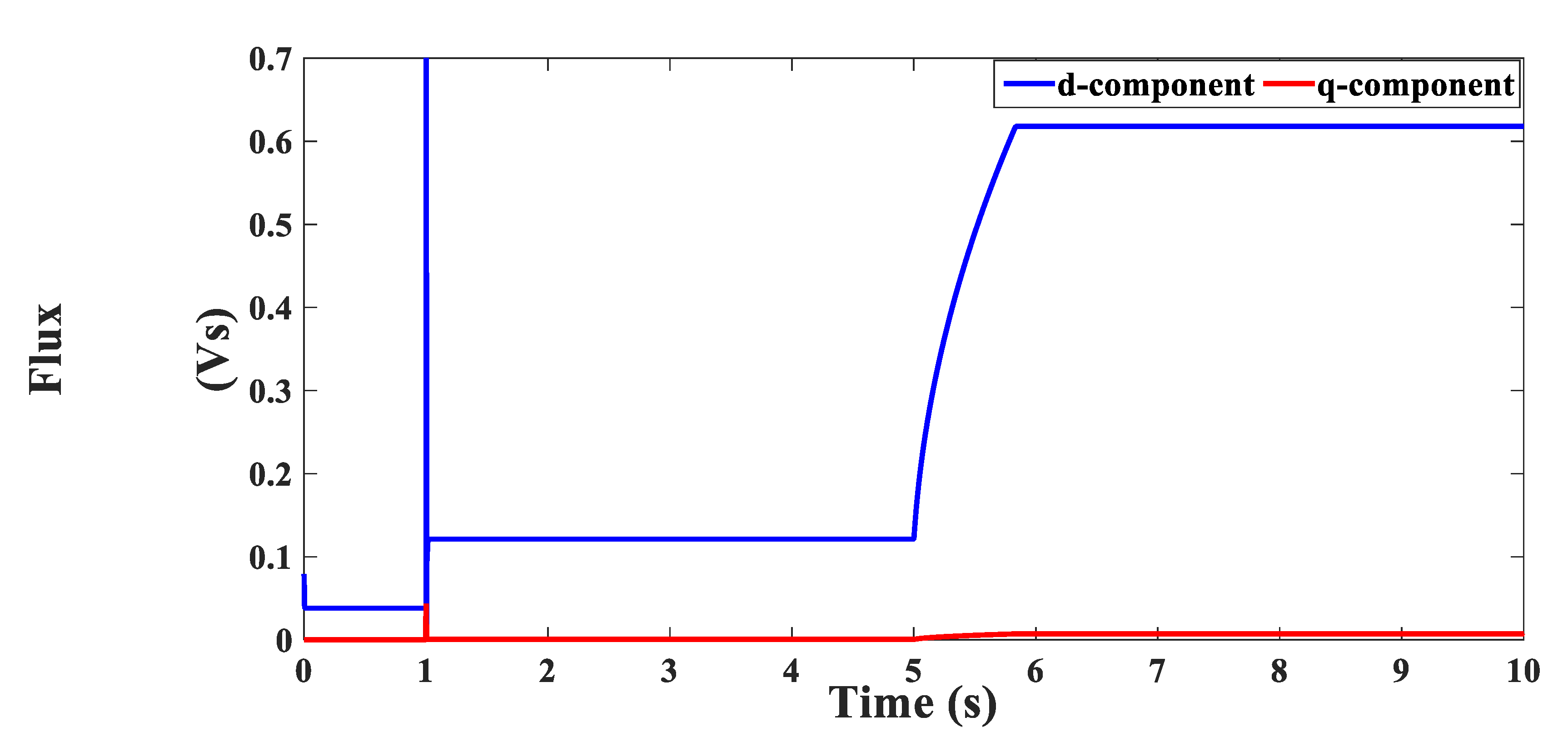
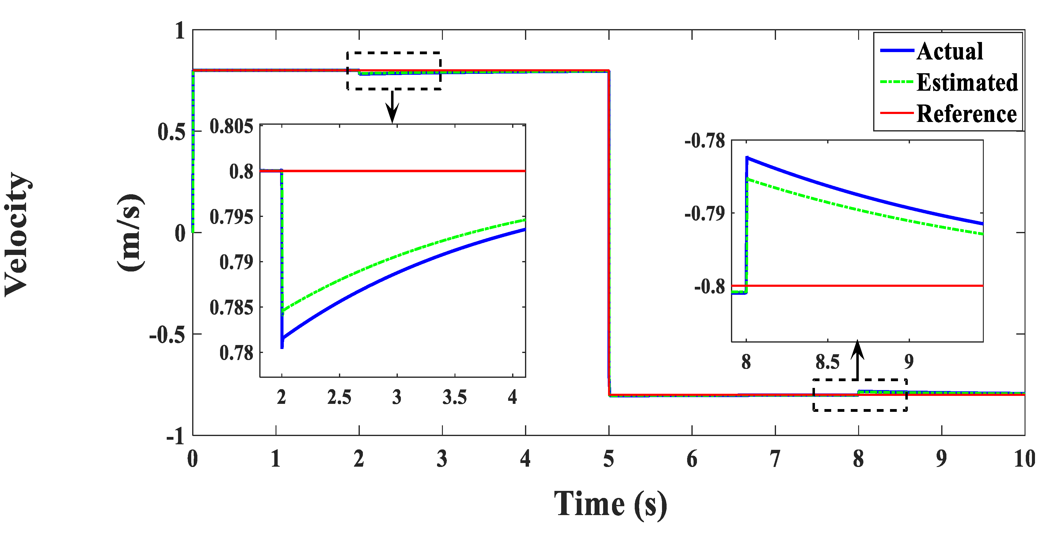
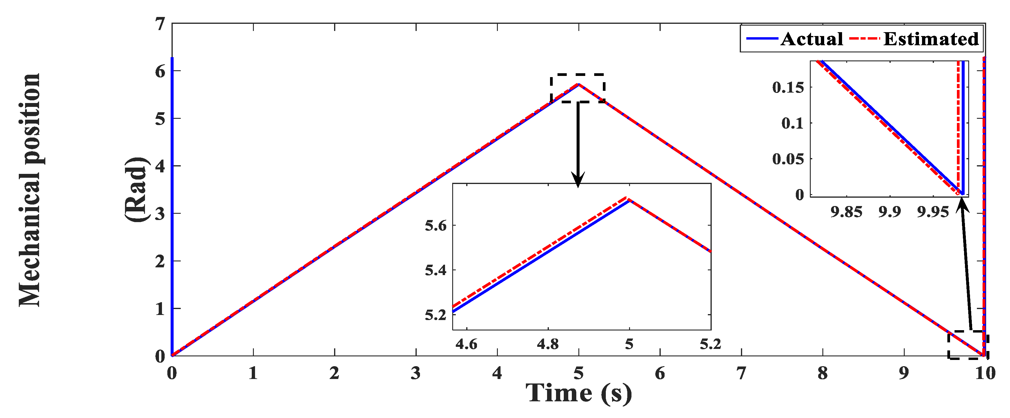
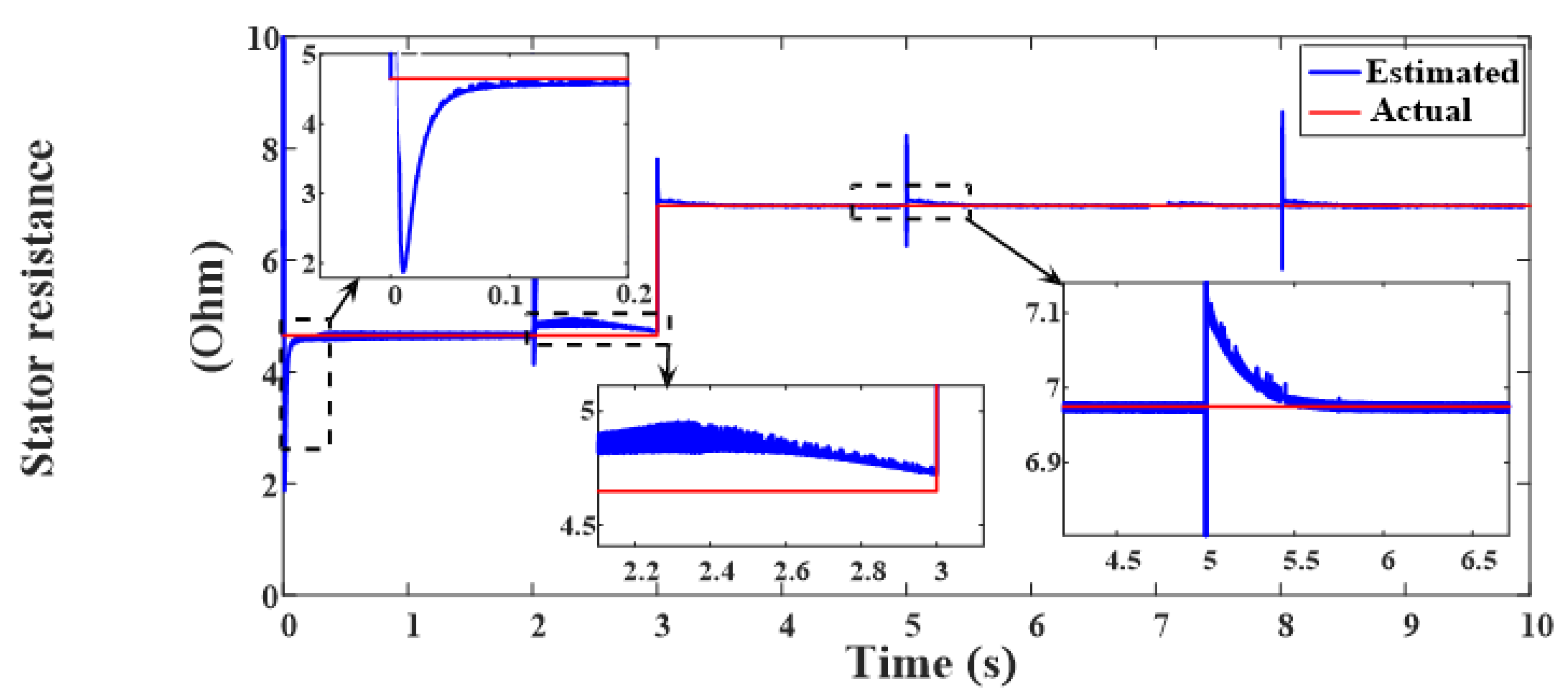
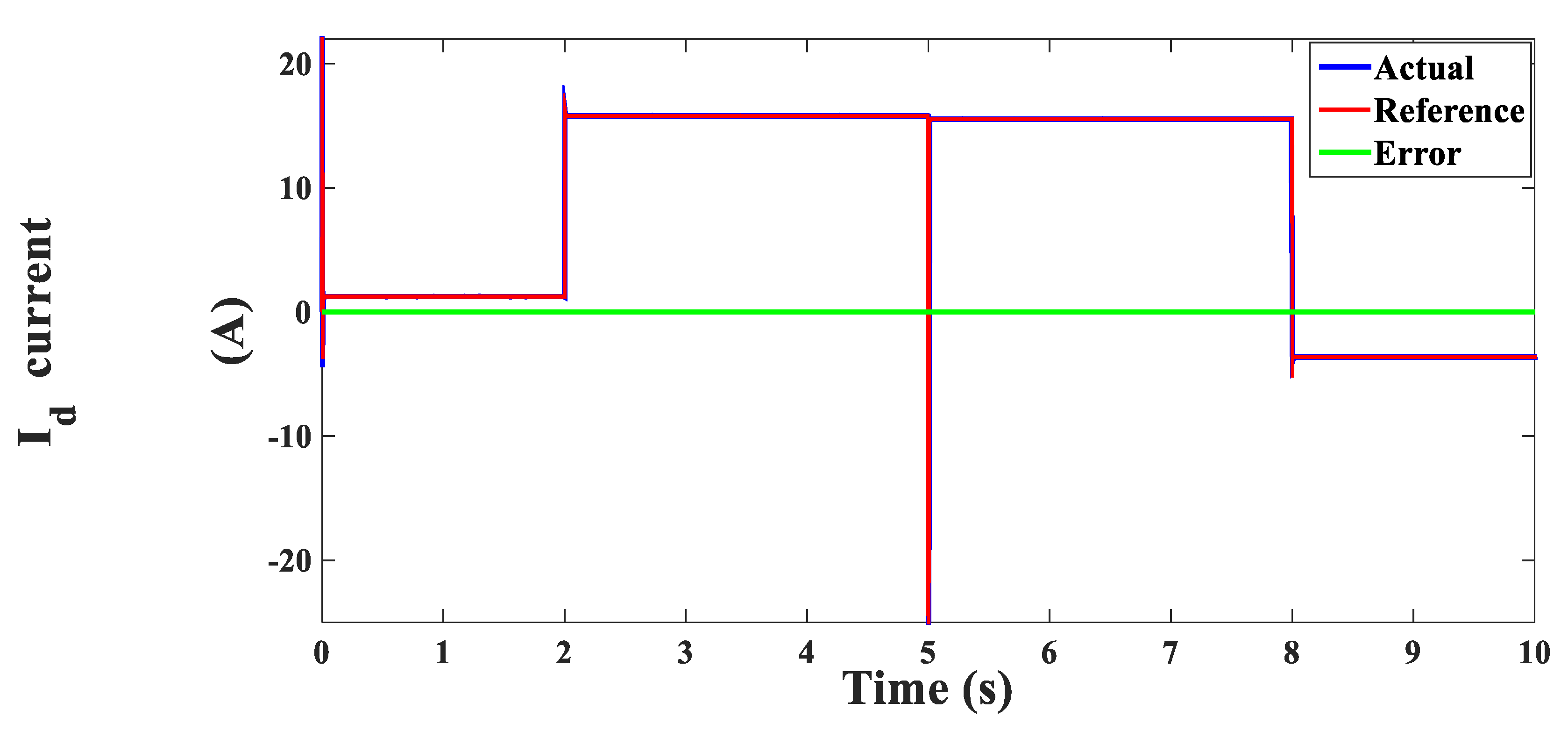
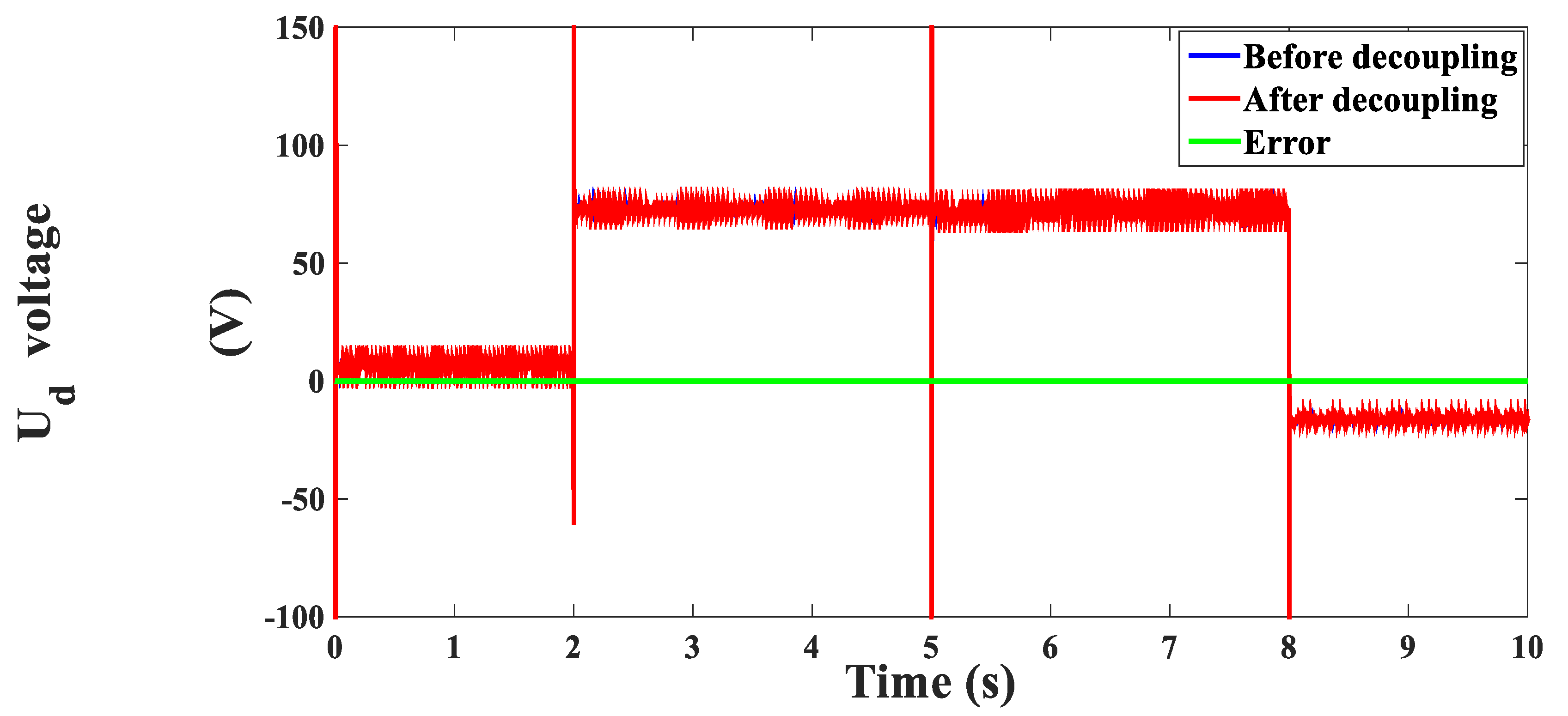
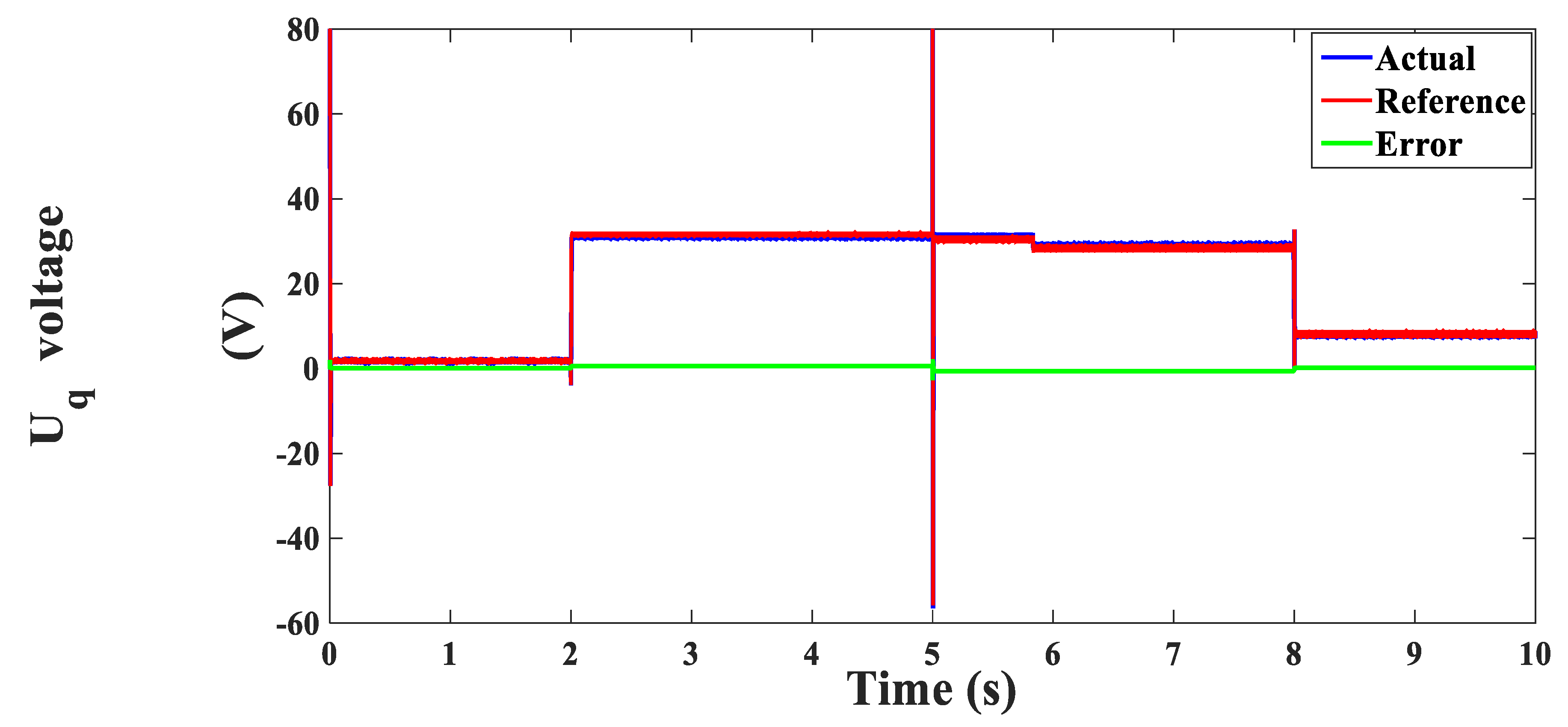
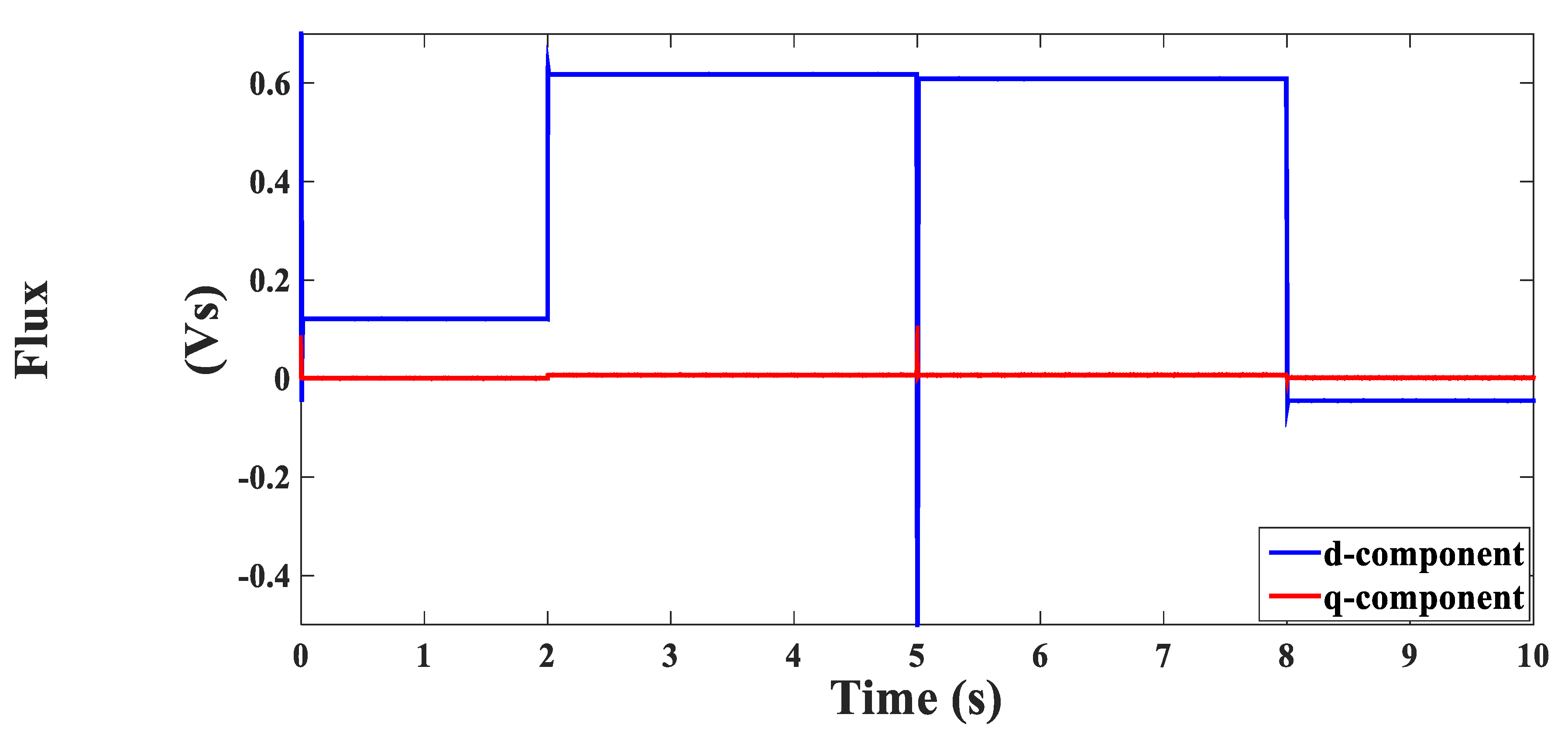
The second test was carried out for a velocity reverse from 0.8 m/s to −0.8 m/s at time t = 5 s. A load force of 25 N was applied at time t = 2 s and removed at time t = 8 s. The obtained results confirmed the validity of the controller in achieving high dynamic behavior under the force and velocity changes. Figure 25 shows the actual and observed velocities, which translated the estimator’s precision. This fact is also confirmed in Figure 26 and Figure 27, which present the real and observed quantities of mechanical position and stator resistance. Figure 28 presents the developed motor’s force and shows that it correctly tracked the load force. Figure 29 and Figure 30 outline the actual d-q stator currents with respect to their references. The currents adeptly accommodated their dynamics according to the applied references. Figure 31 and Figure 32 illustrate the d-q voltage components before and after decoupling. The three-phase voltages are also shown in Figure 33. Furthermore, the d-q flux components are graphed in Figure 34, which shows that a perfect decoupling was realized.
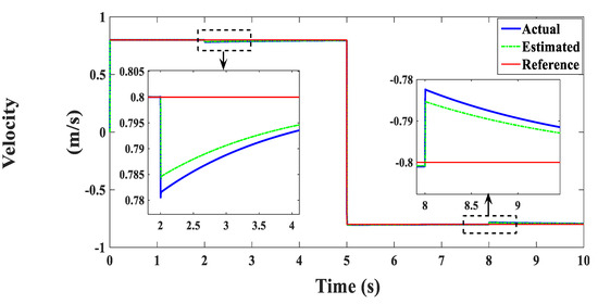
Figure 25.
Motor velocity (m/s).
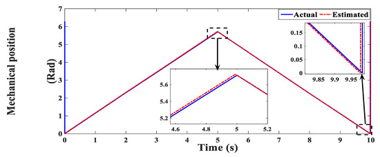
Figure 26.
Mechanical position (Rad).
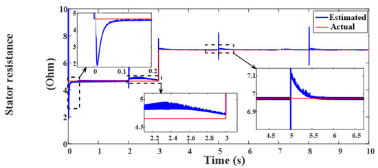
Figure 27.
Resistance variation (Ω).
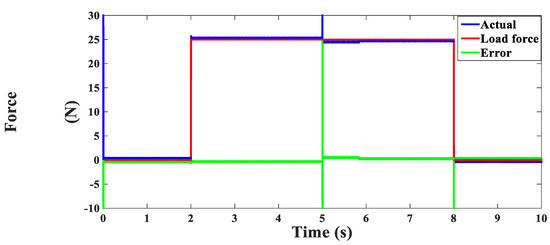
Figure 28.
Motor force (N).
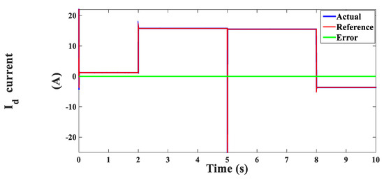
Figure 29.
The d-component of the stator current (A).
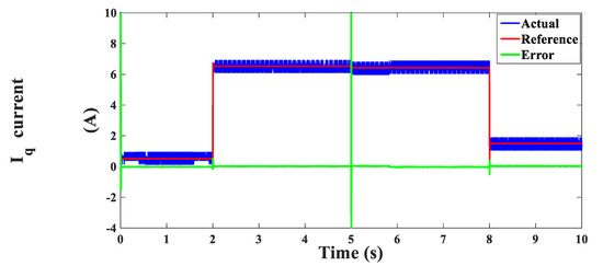
Figure 30.
The q-component of the stator current (A).

Figure 31.
The d-component of the stator voltage (V).

Figure 32.
The q-component of the stator voltage (V).
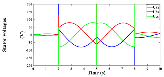
Figure 33.
Stator voltages (V).
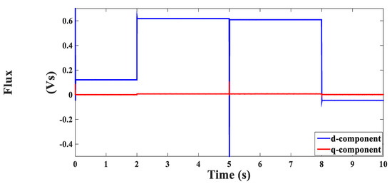
Figure 34.
Flux components (Vs).
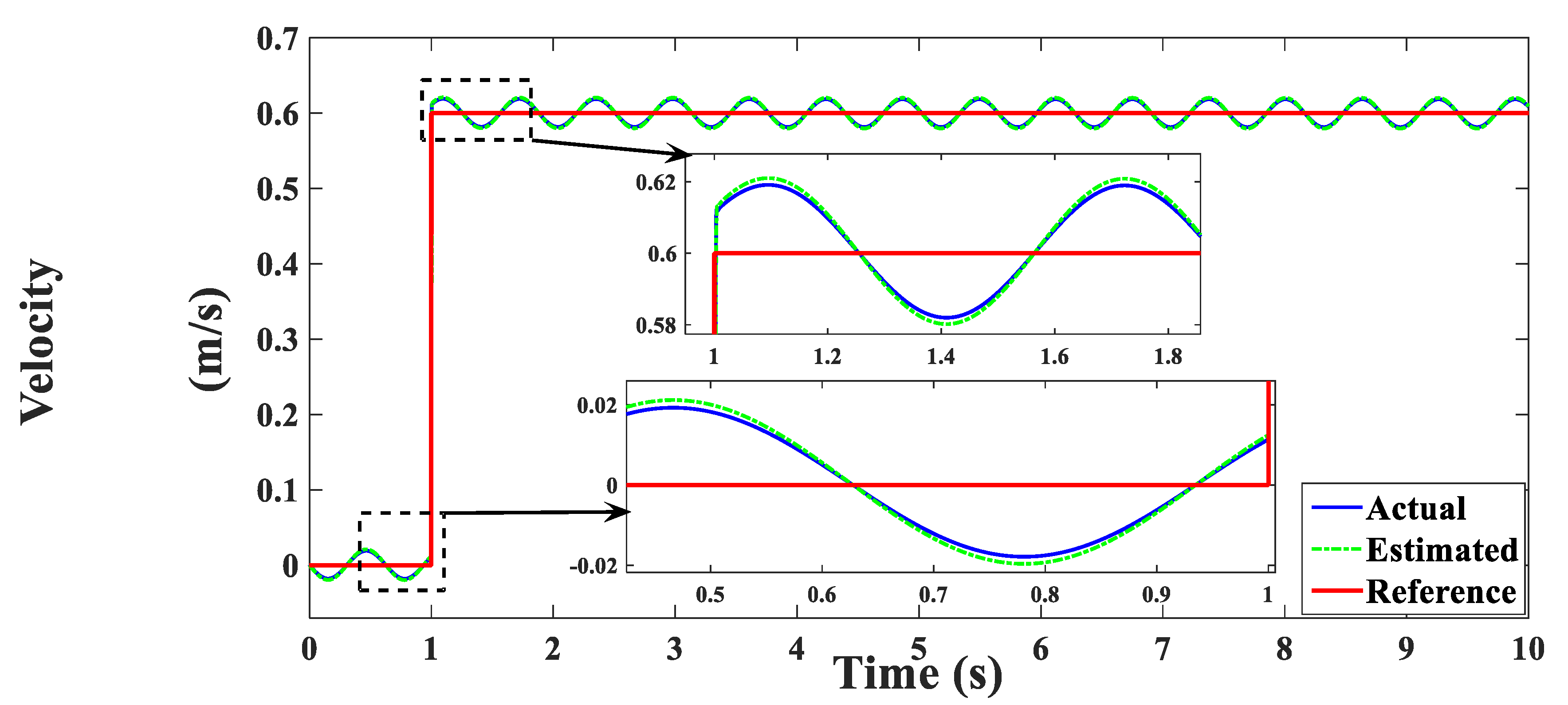
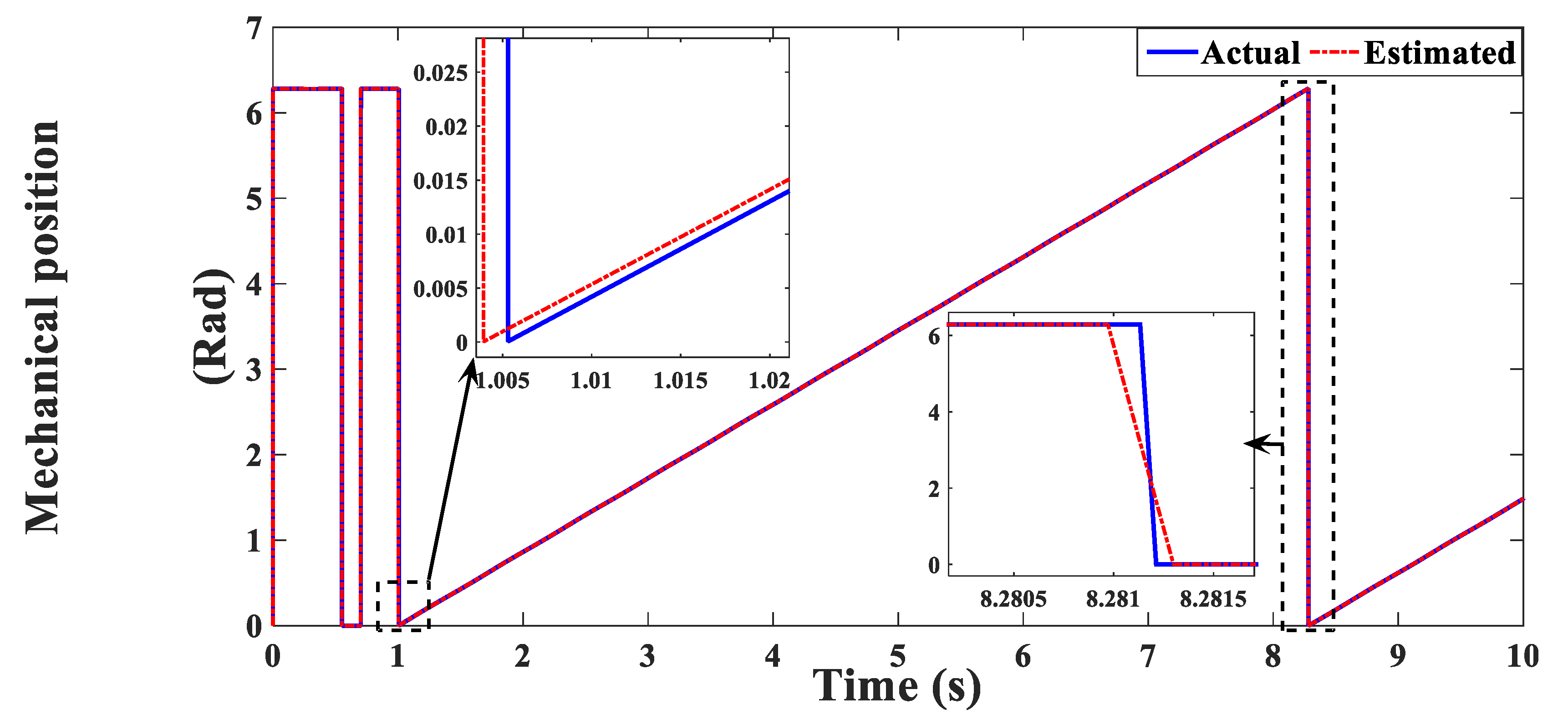
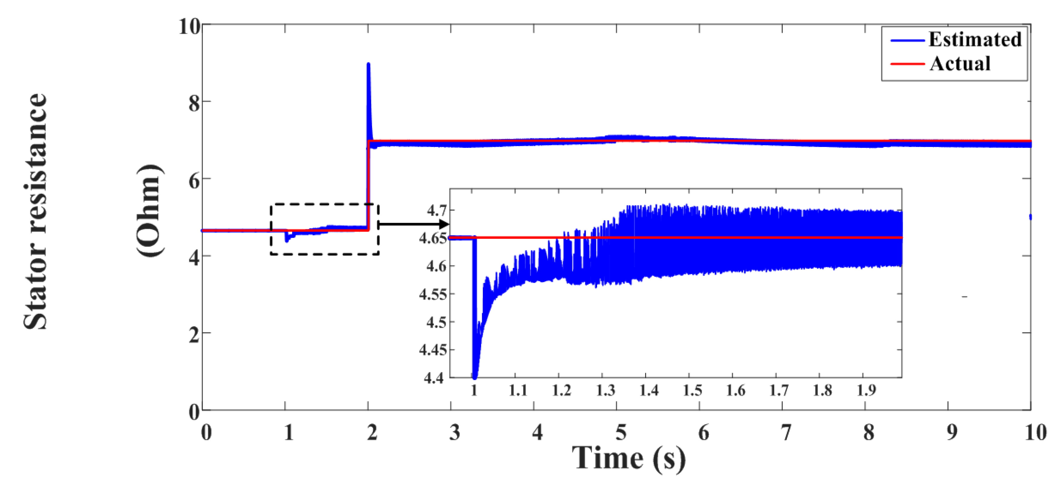
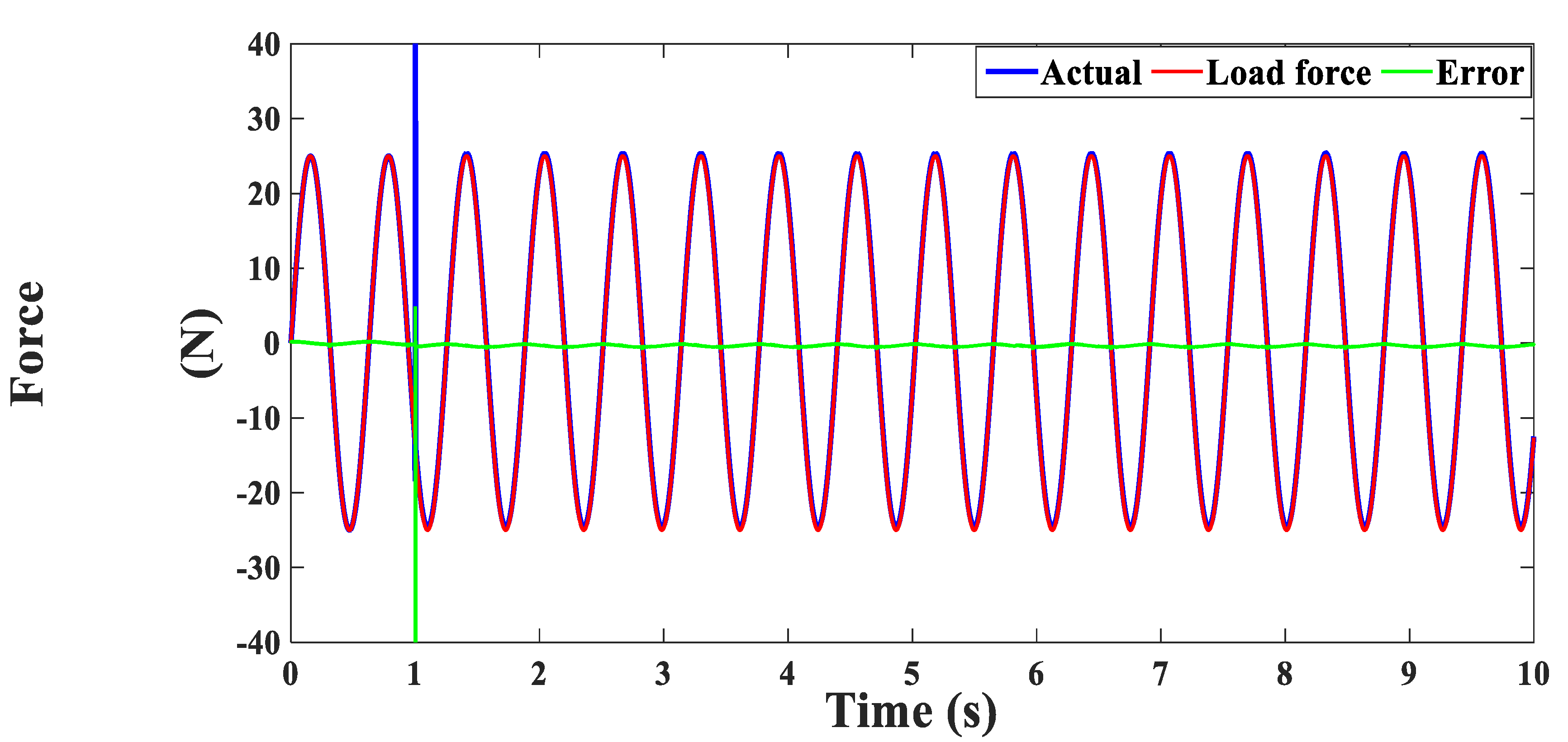
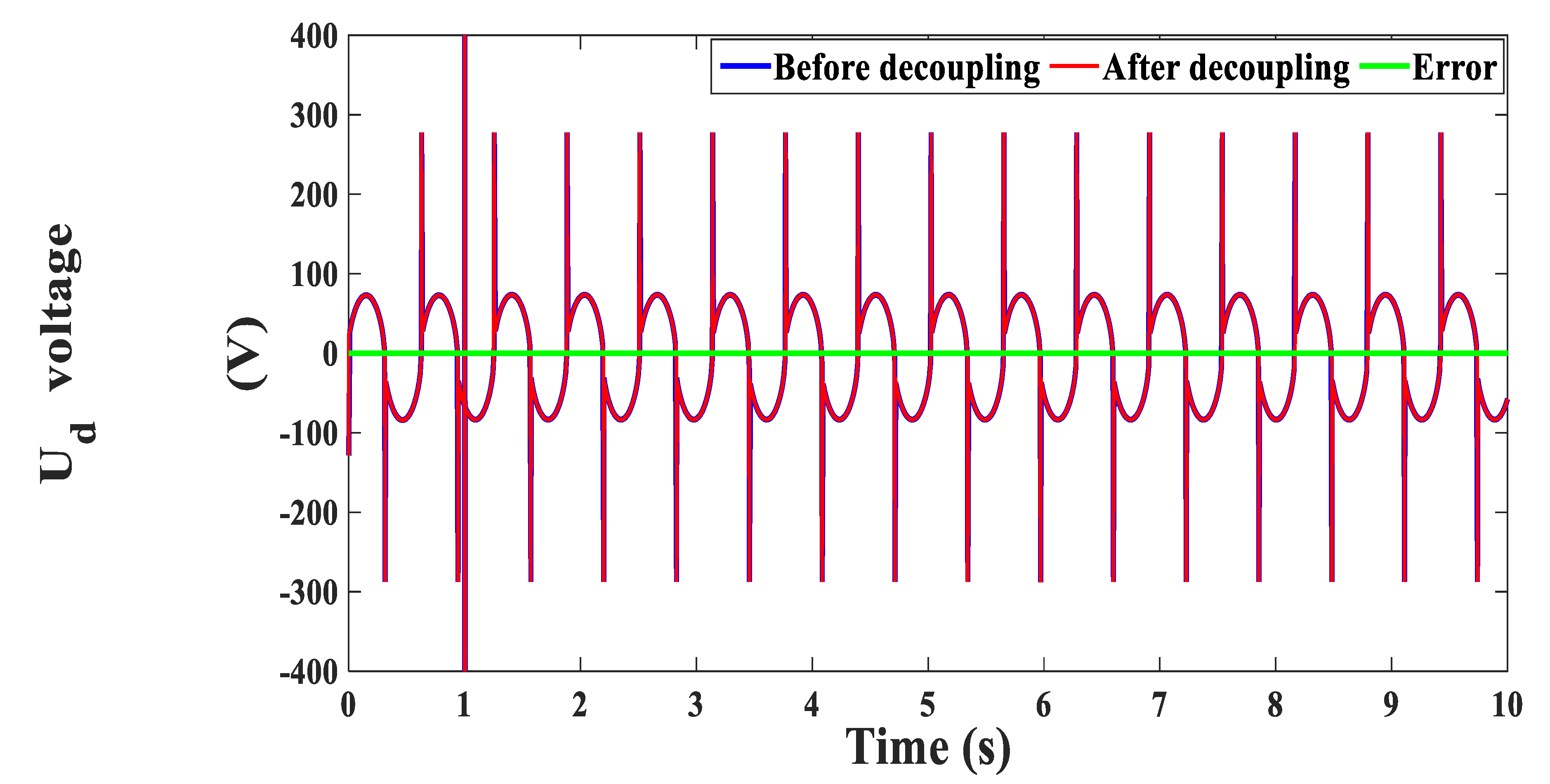
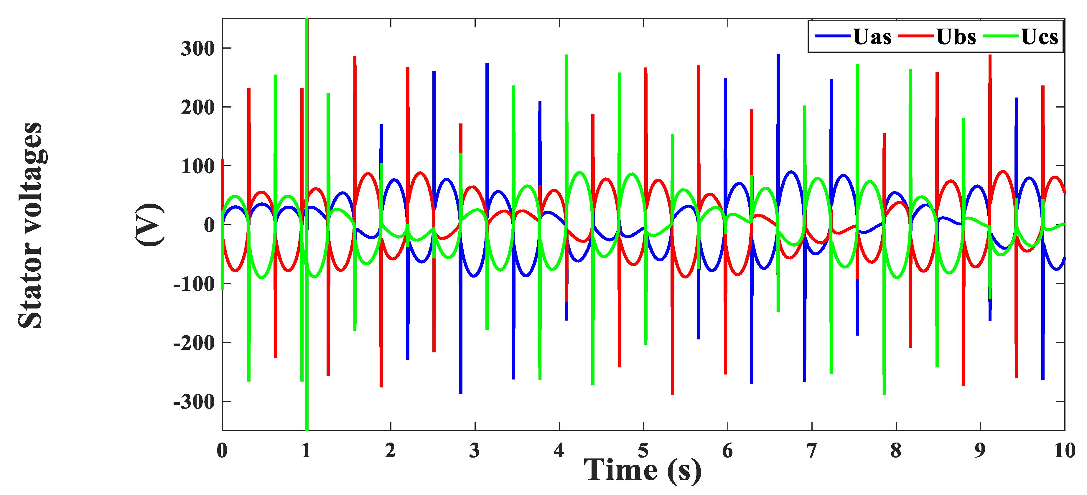
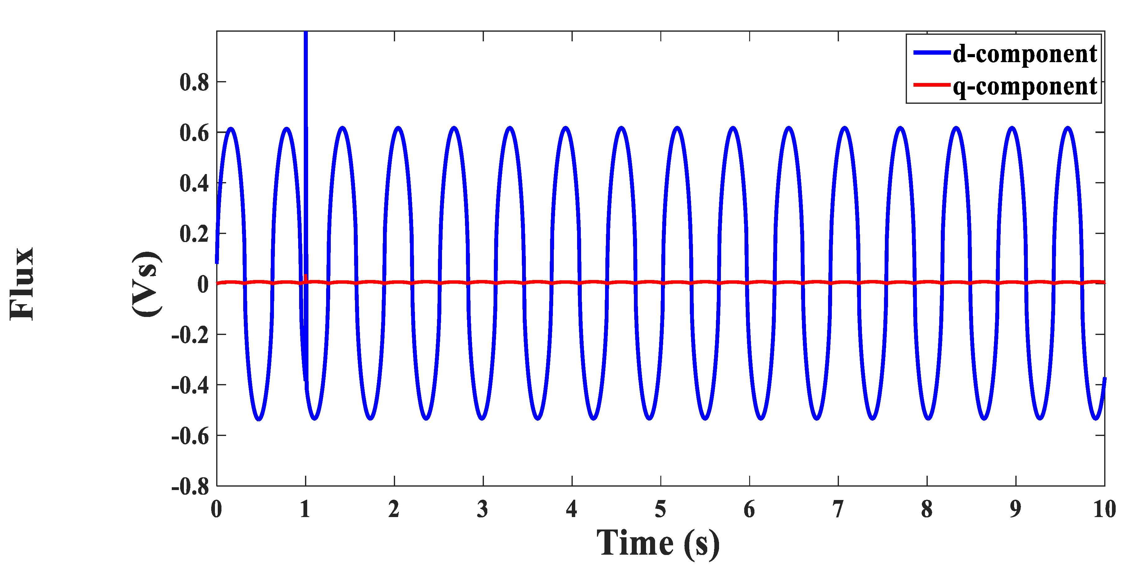
The third test was carried out when applying a reference velocity of 0.6 m/s at time t = 1 s, while applying a load force with sinusoidal waveform with amplitude of 25 Nm. This was made while changing the value of stator resistance by 1.5 times its actual value at time t = 2 s. The sinusoidal load force change was adopted here in order to clarify the validness of the controllers’ design in facing external disturbances. This fact was confirmed through the obtained results as shown in Figure 35, which shows the observed, actual and reference velocities. A very good match was achieved between the actual and estimated signals. Figure 36 and Figure 37 also prove the proper operation of the designed controller and its sensorless mechanism; these two figures show a smooth and concise matching between the real and observed quantities of the cursor’s position and the stator resistance. Figure 38 shows that the developed force exhibited a good tracking of the applied load force. Figure 39 and Figure 40 present the dynamic changes of the stator current d-q components. There was a remarkable precise match between the reference and actual currents. Figure 41 and Figure 42 outline the coupled and decoupled d-q voltage components, and the three-phase voltages are shown in Figure 43. Finally, Figure 44 illustrates that a correct decoupling was achieved between the d-q flux components.
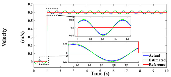
Figure 35.
Motor velocity (m/s).
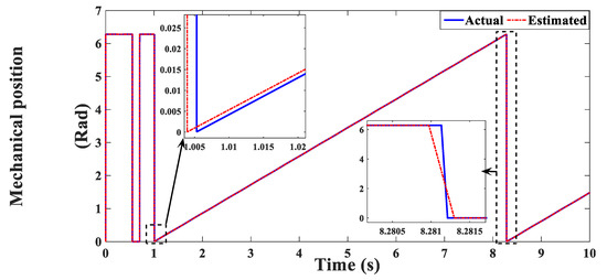
Figure 36.
Mechanical position (Rad).
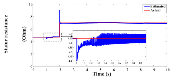
Figure 37.
Resistance variation (Ω).
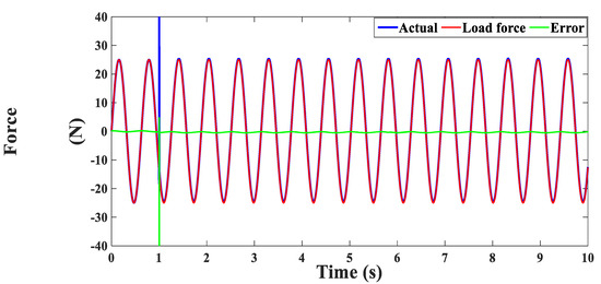
Figure 38.
Motor force (N).
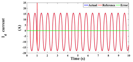
Figure 39.
The d-component of the stator current (A).
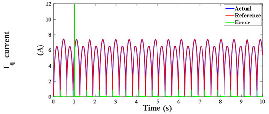
Figure 40.
The q-component of the stator current (A).
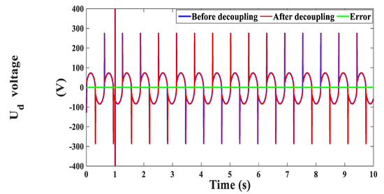
Figure 41.
The d-component of the stator voltage (V).
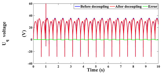
Figure 42.
The q-component of the stator voltage (V).
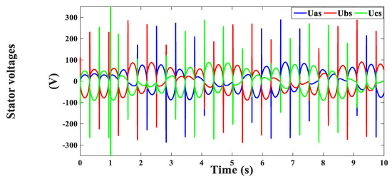
Figure 43.
Stator voltages (V).
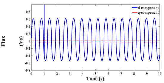
Figure 44.
Flux components (Vs).
6. Conclusions
This paper presented the design and modeling of a robust sensorless control system for a linear tubular-homopolar PMSM. The design and modeling were accomplished in a sequential manner to enable the understanding of the theoretical base upon which the controller’s operation stands. The designed controller consisted of two main control loops: the velocity and current controls. The transfer functions of the controllers were first derived, and then they were used to tune the regulators. In order to increase the system’s reliability, a simple and effective estimator was designed to observe the velocity and stator resistance. The controller’s performance was tested in different operating regimes and under uncertainties as well. The obtained results confirmed the validity of the designed controller, as well as the robustness of the designed estimator.
Author Contributions
Conceptualization, M.A.M., H.E., Z.M.A.; methodology, M.A.M., H.M.S.; software, M.A.M., H.E., H.M.S.; validation, M.A.M., Z.M.A., H.E.; formal analysis, H.E., M.A.M., Z.M.A., H.M.S.; investigation, Z.M.A., H.E., H.M.S.; resources, M.A.M., H.E.; data curation, M.A.M., Z.M.A., H.M.S.; writing—original draft preparation, M.A.M., H.E., H.M.S.; writing—review and editing, H.M.S., Z.M.A., M.A.M., S.F.A.-G.; visualization, M.A.M., H.E., Z.M.A.; supervision, M.A.M., Z.M.A., M.A., S.F.A.-G.; project administration, M.A.M., Z.M.A., M.A.; funding acquisition, M.A., S.F.A.-G. All authors have read and agreed to the published version of the manuscript.
Funding
This work is funded by Research Groups Program, under Grant number (RGP.1/49/42) at King Khalid University and Taif University Researchers Supporting Project Number (TURSP-2020/146), Taif University, Taif, Saudi Arabia.
Acknowledgments
The authors would like to acknowledge the financial support received from the Deanship of Scientific Research at King Khalid University for funding this work through the Research Groups Program, under Grant number (RGP.1/49/42) and Taif University Researchers Supporting Project Number (TURSP-2020/146), Taif University, Taif, Saudi Arabia.
Conflicts of Interest
The authors declare no conflict of interest.
Appendix A

Table A1.
Parameters of the linear motor.
Table A1.
Parameters of the linear motor.
| Parameters | Value | Parameters | Value |
|---|---|---|---|
| Nominal force | 27 N | Pole pairs | 1 |
| Rated speed | 1 m/s | Windings current density | 9 A/mm2 |
| Nominal voltage (rms) | 80 v | Cursor mass (m) | 0.996 Kg |
| R | 4.65 Ω | Dynamic friction (F) | 0.4980 N |
| Ld | 0.0341 H | Magnetic material | NdFeB |
| Lq | 0.0011 H | ||
| ψm | 0.079 Vs |
References
- Boldea, I. Electric generators and motors: An overview. CES Trans. Electr. Mach. Syst. 2017, 1, 3–14. [Google Scholar] [CrossRef]
- Hellinger, R.; Mnich, P. Linear Motor-Powered Transportation: History, Present Status, and Future Outlook. Proc. IEEE 2009, 97, 1892–1900. [Google Scholar] [CrossRef]
- Yang, W.; Wang, Y.; Zhang, P.; Liu, Y. Potential Development of Linear Motors for Unmanned Air Vehicles. IEEE Trans. Appl. Supercond. 2010, 20, 1856–1859. [Google Scholar] [CrossRef]
- De Bruyn, B.; Jansen, J.; Lomonova, E. Comparison of Force Density of Various Superconducting Linear Motor Types Considering Numerically Evaluated AC Losses. IEEE Trans. Appl. Supercond. 2016, 26, 1–5. [Google Scholar] [CrossRef]
- Budig, P. The Application of Linear Motors. In Proceedings of the IEEE Power Electronics and Motion Control Conference Proceedings, Beijing, China, 15–18 August 2000; Volume 3, pp. 1336–1341. [Google Scholar]
- Pandian, S.; Takemura, F.; Hayakawa, Y.; Kawamura, S. Control Performance of an Air Motor—Can Air Motors Replace Electric Motors. In Proceedings of the 1999 IEEE International Conference on Robotics and Automation, Detroit, MI, USA, 10–15 May 1999; pp. 518–524. [Google Scholar]
- Takemura, F.; Pandian, S.; Nagase, Y.; Mizutani, H.; Hayakawa, Y.; Kawamura, S. Control of a Hybrid Pneumatic/Electric Motor. In Proceedings of the 2000 IEEE/RSI International Conference on Intelligent Robots and Systems, Takamatsu, Japan, 30 October–5 November 2000; pp. 209–214. [Google Scholar]
- Lovchik, C.; Diftler, M. The Robonaut Hand: A Dexterous Robot Hand for Space. In Proceedings of the IEEE International Conference on Robotics and Automation, Detroit, MI, USA, 10–15 May 1999; Volume 2, pp. 907–912. [Google Scholar]
- Liang, K. A review of linear compressors for refrigeration. Int. J. Refrig. 2017, 84, 253–273. [Google Scholar] [CrossRef]
- Kwon, Y.; Kim, W. Steady-State Modeling and Analysis of a Double-Sided Interior Permanent-Magnet Flat Linear Brushless Motor with Slot-Phase Shift and Alternate Teeth Windings. IEEE Trans. Magn. 2016, 52, 1–11. [Google Scholar] [CrossRef]
- Hassan, A.; Bijanzad, A.; Lazoglu, I. Dynamic Analysis of a Novel Moving Magnet Linear Actuator. IEEE Trans. Ind. Electron. 2017, 64, 3758–3766. [Google Scholar] [CrossRef]
- Tsai, N.-C.; Chiang, C.-W. High-Frequency Linear Compressor and Lateral Position Regulation. IEEE Trans. Control. Syst. Technol. 2011, 20, 127–138. [Google Scholar] [CrossRef]
- Latham, J.; McIntyre, M.L.; Mohebbi, M. Parameter Estimation and a Series of Nonlinear Observers for the System Dynamics of a Linear Vapor Compressor. IEEE Trans. Ind. Electron. 2016, 63, 6736–6744. [Google Scholar] [CrossRef]
- Park, J.; Park, I.; Cha, J.; Jeong, S. Experimental Investigation of Superconducting Linear Compressor (SCLC) for Pulse Tube Refrigerator (PTR). IEEE Trans. Appl. Supercond. 2017, 27, 1–5. [Google Scholar] [CrossRef]
- Abdalla, I.; Ibrahim, T.; Nor, N. Linear permanent magnet motor for reciprocating compressor applications. In Proceedings of the IEEE 7th International Power Engineering and Optimization Conference (PEOCO), Langkawi, Malaysia, 3–4 June 2013; pp. 29–34. [Google Scholar]
- Wang, J.; Howe, D.; Lin, Z. Design optimization of short-stroke single-phase tubular permanent-magnet motor for refrigeration applications. IEEE Trans. Indus. Electron. 2010, 57, 327–334. [Google Scholar] [CrossRef]
- Wang, J.; Ibrahim, T.; Howe, D. Prediction and Measurement of Iron Loss in a Short-Stroke, Single-Phase, Tubular Permanent Magnet Machine. IEEE Trans. Magn. 2010, 46, 1315–1318. [Google Scholar] [CrossRef]
- Abdalla, I.; Ibrahim, T.; Nor, N. A Study on Different Topologies of the Tubular Linear Permanent Magnet Motor Designed for Linear Reciprocating Compressor Applications. Appl. Comput. Electromagn. Soc. J. 2016, 31, 85–91. [Google Scholar]
- “World First Eco Pedal Helps Reduce Fuel Consumption,” Nissan Eco Pedal System to be Commercialized by 2009. Available online: http://www.nissan-global.com/EN/NEWS/2008/_STORY/080804-02-e.html (accessed on 4 August 2008).
- Pan, J.F.; Cheung, N.C.; Zou, Y. Design and Analysis of a Novel Transverse-Flux Tubular Linear Machine with Gear-Shaped Teeth Structure. IEEE Trans. Magn. 2012, 48, 3339–3343. [Google Scholar] [CrossRef]
- Baoquan, K.; Liyi, L.; Chengming, Z. Analysis and Optimization of Thrust Characteristics of Tubular Linear Electromagnetic Launcher for Space-Use. IEEE Trans. Magn. 2009, 45, 250–255. [Google Scholar] [CrossRef]
- Tomczuk, B.; Sobol, M. Field analysis of the magnetic systems for tubular linear reluctance motors. IEEE Trans. Magn. 2005, 41, 1300–1305. [Google Scholar] [CrossRef]
- Wang, Q.; Zhao, B.; Zhao, H.; Li, Y.; Zou, J. Optimal Design of Tubular Transverse Flux Motors with Low Cogging Forces for Direct Drive Applications. IEEE Trans. Appl. Supercond. 2016, 26, 1–5. [Google Scholar] [CrossRef]
- Zou, Y.; Cheng, K.W.E. Design and Optimization of a Homopolar Permanent-Magnet Linear Tubular Motor Equipped with the E-Core Stator. IEEE Access 2019, 7, 134514–134524. [Google Scholar] [CrossRef]
- Chen, H.; Zhao, S.; Wang, H.; Nie, R. A Novel Single-Phase Tubular Permanent Magnet Linear Generator. IEEE Trans. Appl. Supercond. 2020, 30, 1–5. [Google Scholar] [CrossRef]
- Gu, B.; Kim, Y.; Jung, I.; An, J.; Noh, J. Design and force control of slotted tubular linear motor for active pedal. In Proceedings of the IEEE Energy Conversion Congress and Exposition, Phoenix, AZ, USA, 16–21 September 2011; pp. 1423–1427. [Google Scholar]
- Thomas, J.; Hansson, A. Speed Tracking of a Linear Induction Motor-Enumerative Nonlinear Model Predictive Control. IEEE Trans. Control. Syst. Technol. 2012, 21, 1956–1962. [Google Scholar] [CrossRef]
- Qiwei, X.; Cui, S.; Zhang, Q.; Song, L.; Li, X. Research on a New Accurate Thrust Control Strategy for Linear Induction Motor. IEEE Trans. Plasma Sci. 2015, 43, 1321–1325. [Google Scholar] [CrossRef]
- Karimi, H.; Vaez-Zadeh, S.; Salmasi, F.R. Combined Vector and Direct Thrust Control of Linear Induction Motors with End Effect Compensation. IEEE Trans. Energy Convers. 2016, 31, 196–205. [Google Scholar] [CrossRef]
- Shao, K.; Zheng, J.; Huang, K.; Wang, H.; Man, Z.; Fu, M. Finite-Time Control of a Linear Motor Positioner Using Adaptive Recursive Terminal Sliding Mode. IEEE Trans. Ind. Electron. 2019, 67, 6659–6668. [Google Scholar] [CrossRef]
- El-Sousy, F.F.M.; Abuhasel, K.A. Nonlinear Robust Optimal Control via Adaptive Dynamic Programming of Permanent-Magnet Linear Synchronous Motor Drive for Uncertain Two-Axis Motion Control System. IEEE Trans. Ind. Appl. 2020, 56, 1940–1952. [Google Scholar] [CrossRef]
- Pan, J.; Fu, P.; Niu, S.; Wang, C.; Zhang, X. High-Precision Coordinated Position Control of Integrated Permanent Magnet Synchronous Linear Motor Stations. IEEE Access 2020, 8, 126253–126265. [Google Scholar] [CrossRef]
- Zhao, J.; Wang, L.; Dong, F.; He, Z.; Song, J. Robust High Bandwidth Current Regulation for Permanent Magnet Synchronous Linear Motor Drivers by Using Two-Degree-of-Freedom Controller and Thrust Ripple Observer. IEEE Trans. Ind. Electron. 2020, 67, 1804–1812. [Google Scholar] [CrossRef]
- Liu, X.; Zhen, S.; Sun, H.; Zhao, H. A Novel Model-Based Robust Control for Position Tracking of Permanent Magnet Linear Motor. IEEE Trans. Ind. Electron. 2020, 67, 7767–7777. [Google Scholar] [CrossRef]
- Ji, J.; Xue, R.; Zhao, W.; Tao, T.; Huang, L. Simplified Three-Vector-Based Model Predictive Thrust Force Control with Cascaded Optimization Process for a Double-Side Linear Vernier Permanent Magnet Motor. IEEE Trans. Power Electron. 2020, 35, 10681–10689. [Google Scholar] [CrossRef]
- Accetta, A.; Cirrincione, M.; Pucci, M.; Vitale, G. Neural Sensorless Control of Linear Induction Motors by a Full-Order Luenberger Observer Considering the End Effects. IEEE Trans. Ind. Appl. 2014, 50, 1891–1904. [Google Scholar] [CrossRef]
- Ji, J.; Jiang, Y.; Zhao, W.; Chen, Q.; Yang, A. Sensorless Control of Linear Vernier Permanent-Magnet Motor Based on Improved Mover Flux Observer. IEEE Trans. Power Electron. 2020, 35, 3869–3877. [Google Scholar] [CrossRef]
- Hussain, H.; Toliyat, H. Position sensorless control of a permanent magnet linear motor connected through a long cable. In Proceedings of the IEEE Energy Conversion Congress and Exposition (ECCE), Cincinnati, OH, USA, 1–5 October 2017; pp. 830–835. [Google Scholar]
- Cao, R.; Jiang, N.; Lu, M. Sensorless Control of Linear Flux-Switching Permanent Magnet Motor Based on Extended Kalman Filter. IEEE Trans. Ind. Electron. 2020, 67, 5971–5979. [Google Scholar] [CrossRef]
- Wang, H.; Yang, Y.; Ge, X.; Li, S.; Zuo, Y. Speed-Sensorless Control of Linear Induction Motor Based on the SSLKF-PLL Speed Estimation Scheme. IEEE Trans. Ind. Appl. 2020, 56, 4986–5002. [Google Scholar] [CrossRef]


Publisher’s Note: MDPI stays neutral with regard to jurisdictional claims in published maps and institutional affiliations. |
© 2021 by the authors. Licensee MDPI, Basel, Switzerland. This article is an open access article distributed under the terms and conditions of the Creative Commons Attribution (CC BY) license (https://creativecommons.org/licenses/by/4.0/).