Detection of Diseases in Tomato Leaves by Color Analysis

Abstract

Agricultural productivity is an important factor for the economic development of a country. Therefore, the diagnosis of plant diseases is a field of research of utmost importance for the agricultural sector as it allows us to help recommend strategies to avoid the spread of diseases, thus reducing economic losses. Currently, with the rise of computer systems, computer systems have been developed that allow computer-assisted diagnosis in different research fields, including the agricultural sector. This work proposes the development of a methodology that allows the detection of three types of diseases in tomato leaves (late blight, tomato mosaic virus and Septoria leaf spot) by image analysis and pattern recognition. The methodology is divided into three stages: (1) segmentation of the leaf and of the lesion, (2) feature extraction using color moments and Gray Level Co-occurrence Matrix (GLCM) and (3) classification. For the segmentation process, it is proposed to use a range of pixel colors that represent healthy and diseased areas in tomato leaves using values proposed by an expert in the area of phytopathology. For the classification it is proposed to use a decision rule in which if two of the Support Vector Machines (SVM) classifiers, K Nearest Neighbors (K-NN) and Multilayer Perceptron (MLP) give the same result, then this is taken for the final decision. The result of the methodology is compared with other classifiers using the value of its accuracy and validated with cross validation.

1. Introduction

According to the Food and Agriculture Organization (FAO) data, the global tomato area grew at an average annual rate of 1.4% between 2007 and 2017, to reach 4.8 million hectares. Of the total area harvested in 2017, this was concentrated in five countries: China with 21.2%, India with 16.4%, Nigeria with 12.2%, Turkey with 3.9% and Egypt with 3.8% [1,2]. According to statistics from the National Institute of Food and Agriculture (U.S.A), crops worldwide, between 40 and 50%, are lost, caused by pests and different crop diseases, so monitoring and the detection of plant diseases is of utmost importance for sustainable agricultural development [3]. Detecting plant diseases by manual monitoring is slow work that requires the preparation of an expert in the agricultural area. However, with the growth of computer systems, and mainly in the development of the field of machine learning, studies have been carried out to detect diseases in plants automatically [4,5,6]. Late blight is one of the most devastating diseases that infects tomatoes, potatoes and other nightshades. Late blight is caused by the oomycete Phytophthora infestans, the first symptoms of which are shown as watery or oily lesions on the leaves that later turn into a purple and brown color, and later the appearance of mycelium, infecting stems and fruits. Late blight was the main cause of the Great Irish famine from 1845 to 1849 and of the Great Scottish Famine of 1846 to 1857 [7,8]. Tomato mosaic virus belongs to the genus Tobamovirus [9]; this virus is present worldwide, causing heavy damage to tomato crops grown both outdoors and those that are under protection. The main symptom consists of alterations in the shape and color of the leaves, with chlorotic areas and others of normal green and dark green color (mosaics) with upward curl [10]. On the other hand, leaf spot is caused by the pathogenic fungus Septoria lycopersici [11], which is characterized by small circular spots of up to 3 mm in diameter, with white centers and black edges, lesions very similar to those caused by late blight. At a very advanced stage, the area affected by the fungus is clearly visible [12].

Various methodologies have been developed that allow the detection of diseases in plants [13,14]. Some of these perform manual segmentation of the damaged areas [13], while others make use of deep learning applied directly to the image color [14,15], leaving aside the segmentation process. In this work, an automated methodology is proposed using methods in the spatial domain, and it is proposed to use a range of values of the pixels that represent healthy and diseased areas in tomato leaves, through values exposed by an expert in the area of phytopathology for the segmentation process in such a way that it is possible to visualize the damaged areas in tomato leaves. On the other hand, there are studies that only focus on the detection of a particular disease such as late blight [16,17] or Septoria leaf spot [18]. The work proposal addresses three types of diseases in tomato leaves: late blight, Septoria leaf spot and mosaic virus in tomato leaves. There are works that specialize in the detection of various diseases in plants [15,19,20] without considering the class of healthy leaves, while in this research two classifications are considered; firstly, it is detected if a tomato leaf is found healthy or diseased, and secondly, if a leaf is diseased, then it is detected which type of disease it suffers from, among the three considered. Some studies propose extracting characteristics such as color and shape from images of plant lesions [21,22]. In this study, for the extraction of characteristics, four color moments are used for each RGB component and nine statistical measures are used for texture analysis by GLCM, as shown in [23,24]. Most of the architectures shown in the works make use of a classifier model in a sequential way to test using algorithms such as ANN [25], SVM [26] and K-means [27] among others; however, some works propose to carry out an architecture in which the classification depends on three algorithms such as FIS, ANFIS and MLP [28]. In this research, it is also proposed to use three classifier models in parallel (MLP, K-NN and SVM) considering a decision rule that suggests that, if two classifiers give the same result, then this will be the final result.

This article is structured as follows. Section 1 shows the introduction. In Section 2 the necessary tools for the development of the work are presented. Section 3 shows the proposed methodology. In Section 4 the experiments and results are presented. In Section 5 the discussion of results is presented. Finally, in Section 6 the conclusions are presented.

2. Materials and Methods

2.1. Image Acquisition

Imaging is a process by which 3D light information (scene) is projected onto a 2D plane (digital image). To carry out this process, an optical sensor is needed. An optical sensor is an electrical or electrochemical sensor that allows data to be obtained digitally from analog data. The optical sensor is composed of a matrix of small microscopic photosensitive cells aligned in rows and columns, each of these cells producing electrical impulses of different intensities depending on the amount of light they receive. The information obtained by an optical sensor (different levels of electrical current for each cell) is processed by an analog to digital signal converter (ADC), obtaining digital data as an output that is represented by pixels. Pixels are generally organized in an ordered rectangular array. The size of an image is determined by the dimensions of this pixel array. The width of the image is the number of columns $W$, and the height of the image is the number of rows $H$ of the array. Therefore, the pixel array is an array of size $H\times W$. To refer to a specific pixel within the array of an image, it will be done using its coordinate $\left(x, y\right)$. In addition, each pixel position $\left(x, y\right)$ has an associated color intensity that will be denoted as $I_{xy}=I\left(x, y\right)$. Figure 1 shows the process for acquiring a digital image from the 3D scene.

2.2. Color Models

Color pixel handling is of utmost importance in image processing, due to the characteristics that allow highlighting in the image, such as brightness, chromaticity, intensity of a certain color, etc. There are different color models, and one of the most common is the RGB (Red-Green-Blue) model. The RGB model is based on a cartesian coordinate system where the color subspace of interest is the cube, and the colors are defined by a point in space where their coordinates $\left(x, y, z\right)$ represent the red color, green and blue, respectively. On the other hand, the HSV (Hue, Saturation, Value) model is represented by an inverted cone. The $H$ component is the circular region with values between 0° and 360°, and the $S$ and $V$ components are represented on the horizontal and vertical axes, respectively, as shown in Figure 2.

To carry out the conversion from the RGB model to the HSV model, the values of the RGB channels are obtained on a scale of 0 to 1, that is, $R=\frac{R^{\prime }}{scal{e}_r}$, $G=\frac{G^{\prime }}{scal{e}_g}$ and $B=\frac{B^{\prime }}{scal{e}_b}$, where the scale variable represents the scale of the channel, in this case, of 255. In this way, $m_{max}=max\left(R, G, B\right),min=min\left(R, G, B\right)\mathrm{and} \Delta =m_{max} – m_{min}$ are defined. Then,

$$H=\{\begin{array}{ll}undefined,& if \Delta =0\\ \frac{G-B}{\Delta },& if m_{max}=R\\ \frac{B-R}{\Delta }+2,& if m_{max}=G\\ \frac{R-G}{\Delta }+4,& if m_{max}=B\end{array}$$

(1)

$$V=m_{max}$$

(2)

$$S=\{\begin{array}{c}0, if V=0\\ \frac{\Delta }{V}, otherwise\end{array}$$

(3)

$H^{\prime }=H\times scal{e}_h, S^{\prime }=S\times scal{e}_s \mathrm{and} V^{\prime }=V\times scal{e}_v$, where $scal{e}_h,$ $scal{e}_s$ and $scal{e}_v$ represent the scale of the HSV channels.

2.3. Image Histogram

The histogram of a digital image with gray levels in the range [0, 255] is a discrete function $Histo \left[k\right]$ that represents the number of colors for each gray level $(k=0,\dots ,255$). The graphical representation of this function for all values of $k$ provides an overall description of the appearance of the image [29]. Although the histogram does not indicate something specific about the content of the image, it provides us very useful information on the possibility of highlighting interesting features of the image.

2.4. Otsu Method

The Otsu method is to split an image into gray levels with $N$ pixels and $L$ different possible levels. The probability of occurrence of the gray level $i$ in the image is given by $p_i=f_i/N$, with $f_i$ the frequency of repetition of the $i$-th gray level $\left(i=1, 2,\dots , L\right)$. Consider ${\omega }_1={\sum }_{i=1}^t{p}_i \mathrm{and} {\omega }_2={\sum }_{i=t+1}^L{p}_i, \mathrm{where} 1, 2,\dots , t, \mathrm{and} t+1, t+2,\dots , L$ are the gray levels corresponding to classes $C1$ and $C2$ (binarization), then the probability distributions of classes $C1$ and $C2$ are given, respectively, by

$$\frac{p_1}{{\omega }_1 \left(t\right)}, \frac{p_2}{ \omega { }_1\left(t\right)},\dots , \frac{p_t}{ \omega { }_1\left(t\right)}$$

(4)

and

$$\frac{p_{t+1}}{ \omega { }_2\left(t\right)} , \frac{p_{t+2}}{ \omega { }_2\left(t\right)},\dots , \frac{p_L}{ \omega { }_2\left(t\right)}$$

(5)

The averages for each class are, respectively, defined as

$${\mu }_1={\sum }_{i=1}^t\frac{i{P}_i}{\omega { }_1\left(t\right)}$$

(6)

and

$${\mu }_2={\sum }_{i=t+1}^L\frac{i{P}_i}{\omega { }_2\left(t\right)} .$$

(7)

The variance between classes of a threshold image is given by

$${\sigma }_B^2={\omega }_1{\left({\mu }_1 – \mu T\right)}^2+{\omega }_2{\left({\mu }_2 – \mu T\right)}^2$$

(8)

with

$${\mu }_T={\omega }_1{\mu }_1+{\omega }_2{\mu }_2.$$

(9)

The optimal threshold that maximizes the variance is

$$t^{*}=Ma{x}_t\left\{{\sigma }_B^2\left(t\right)\right\}$$

(10)

2.5. Related Components

An essentially related component is to group pixels from the same region by assigning them the same label. To refine the definition of a related component, consider 8-connectivity. It is said that a pixel $p$ is connected by 8-connectivity to a pixel $q$, if $p$ is one of its 8 neighbors adjacent to $q$. A path from pixel $p$ to pixel $q$ is a sequence of pixels $r_0,r_1,\dots ,r_k$ such that $r_0=p, r_k=q$ and pixel $r_i$ is connected by 8-connectivity to pixel $r_i+1$for each $0\le i\le k$. A region $S$ of an image is a related component if for each pair of pixels $p, q$ in $S$, there is a path from $p$ to $q$ where each pixel that defines the path is also in $S$.

2.6. Support Vector Machines

The Support Vector Machine (SVM) is a statistical method of supervised, controlled and non-parametric learning and operates on the premise that the type of distribution of the data set is unknown. SVM is a binary classification method that takes a set of input data and classifies it into one of two different classes. The power of SVM lies in its ability to transform data into a higher dimensional space than where they are, where the data can be separated by an optimal hyper plane that maximizes the margin distance between the two classes [30,31].

2.7. K-Nearest Neighbor (K-NN)

The K-NN algorithm is a widely used non-parametric method for classification in pattern recognition. The principle of the K-NN algorithm is to determine the class to which an input data belongs from its K closest neighbors. For this, a training set is required $T=\left\{\left(Y_1, C_1\right), \left(Y_2, C_2\right),\dots , \left(Y_n, C_n\right)\right\}$, where $Y_i\in ℝ{ }^d$ and $C_i$ denote the class to which it belongs$Y_i,i=1, 2,\dots , n$. Given an input $X\in ℝ{ }^d$, of which you want to know its class, the Euclidean distance is calculated with each of the data of $T$, that is, $d \left(X, Y_i\right)=\parallel X-Y\parallel$ is calculated for each $i=1, 2,\dots , n$, the K elements of $T$ closest to $X$ are selected via Euclidean distance and their classes are counted, in such a way that $X$will be classified to the class that counts the most votes of the $K$ closest elements [32].

2.8. Multilayer Perceptron (MLP)

MLP is an artificial neural network model (ANN) made up of multiple layers. MLP is composed of an input layer with n nodes, an output layer and m intermediate hidden layers. In the learning phase, MLP uses a technique called backpropagation, in order to modify the weights of the connections between the networks, to obtain an approximation to the expected output data. Each layer consists of an independent process of units called neurons. Each neuron receives inputs, each input value is multiplied by weight. The input is computed using a mathematical function that determines the activation value of the neuron and then goes to the next layer [33].

2.9. GLCM Gray Level Co-Occurrence Matrix and Color Moments

Color moments are very effective for color-based analysis, as the color distribution in-formation of an image can be captured by the low order moments. The color moments used are the first, second, third and fourth order, that is: the average, standard deviation, asymmetry and kurtosis. From these moments, a collection of descriptive measurements is obtained which together form the color features of the image. The four moments of color can be defined as:

Moment 1: Medium. It is the average of the intensity of the pixels. It describes its general character and brightness. Its formula is given by:

$$\mu =\frac{{\sum }_{ij}{I}_{ij}}{N}$$

(11)

where $N$ is the total number of pixels in the image.

Moment 2: Standard deviation. It measures the dispersion of the intensity values with respect to the medium. It indicates how each pixel in the image varies from neighboring or center pixels and the contrast of the image. The standard deviation is obtained using the following statistical formula:

$$\sigma =\sqrt{\frac{{\mathsf{\Sigma }}_{ij}{\left(I_{ij}-\mu \right)}^2}{N}}$$

(12)

Moment 3: Asymmetry. Measure in which the intensity values are not symmetrical with respect to the medium. It indicates the asymmetry of the intensity of the values. Its formula is given by:

$$\frac{{\mathsf{\Sigma }}_{ij}{\left(I_{ij}-\mu \right)}^3}{N{\sigma }^3}$$

(13)

Moment 4: Kurtosis. Measurement that indicates if the intensity distribution is maximum or flat with respect to the normal distribution. Kurtosis is given by:

$$\frac{{\mathsf{\Sigma }}_{ij}{\left(I_{ij}-\mu \right)}^4}{\left(N-1\right){\sigma }^4}$$

(14)

On the other hand, gray level co-occurrence matrices (GLCM) are useful for image texture analysis. GLCM functions characterize the texture of an image by calculating how often pixel pairs with specific values and in a specific spatial relationship are produced in an image, creating a GLCM C matrix, and then extracting statistical measures from this matrix. If $C=\left\{c_{ij}\right\}$ is the GLCM size matrix $N\times N$, then the statistical measures used are:

• Medium:

  $${\mu }_i={\displaystyle \sum }_{i,j=1}^{N}i{c}_{ij},{\mu }_j={\displaystyle \sum }_{i,j=1}^{N}j{c}_{ij}$$

  (15)
• Standard deviation:

  $${\sigma }_i^2={\displaystyle \sum }_{i,j=1}^N{c}_{ij}{\left(i-{\mu }_i\right)}^2$$

  (16)
• Correlation:

  $${\displaystyle \sum }_{i,j=1}^N{c}_{ij}\left[\frac{\left(i-{\mu }_i\right)\left(j-{\mu }_j\right)}{\sqrt{\left({\sigma }_i^2\right)\left({\sigma }_j^2\right)}}\right]$$

  (17)
• Entropy:

  $$-{\displaystyle \sum }_{i=1}^N{\displaystyle \sum }_{j=1}^N{c}_{ij}log{c}_{ij}$$

  (18)
• Dissimilarity:

  $${\displaystyle \sum }_{i=1,j=1}^N{c}_{ij}\left|i-j\right|$$

  (19)
• Contrast:

  $${\displaystyle \sum }_{i=1,j=1}^N{c}_{ij}{\left(i-j\right)}^2$$

  (20)
• Homogeneity:

  $${\displaystyle \sum }_{i=1}^N{\displaystyle \sum }_{j=1}^N\frac{1}{1+{\left(i-j\right)}^2}{c}_{ij}$$

  (21)
• Energy:

  $${\displaystyle \sum }_{i=1}^N{\displaystyle \sum }_{j=1}^N{\left|c_{ij}\right|}^2$$

  (22)
• Maximum probability:

  $$\max \left(c_{ij}\right)$$

  (23)

3. Proposed Model

In this section, the methodology is shown that allows the detection of three tomato leaf diseases: late blight, tomato mosaic and Septoria leaf spot. The methodology is divided into three modules: segmentation, extraction of features and classification.

3.1. Segmentation

The segmentation procedure for obtaining the damaged area in tomato leaves is carried out by means of the following sequence of steps:

• The grayscale image is obtained using the average of the three channels of the RGB model, that is,$I \left(x, y\right)=\frac{R \left(x, y\right)+G \left(x, y\right)+B \left(x, y\right)}{3}$;
• The negative operator $Neg \left(x, y\right)=255-I \left(x, y\right)$ is applied;
• A median filter with a 3 × 3 mask is applied;
• The threshold is set using the Otsu method (Equations (4)–(10)).

The connected components are determined through the 8-connectivity of those areas that have pixels with value equal to 255 (white pixels), and those components with an area less than a threshold equal to 300 pixels are eliminated. This allows us to leave only the connected component that corresponds to the background of the image. The image is then binarized by transforming f (x, y) = 0 if the pixel corresponds to a pixel with a value of 255 (area of the sheet), and f (x, y) = 255 otherwise (background of the image). Once the image is binarized, an and operation is performed with the color input image to obtain the segmented image of the sheet. Figure 3 shows the block diagram to obtain the segmented image of the sheet.

Figure 4 shows the steps applied to obtain the segmented image of the leaf to an image of the PlantVillages image set. Figure 4g shows the area of the sheet in white and the background in yellow that corresponds to the connected component with the largest area. Through the transformation given by f (x, y) = 0 if the pixel corresponds to a white pixel, and f (x, y) = 255 if the pixel corresponds to a background pixel, the binarized image is obtained as in Figure 4h. Finally, an and operation is performed with the color image to obtain the segmented image of the sheet as shown in Figure 4i.

The color space is transformed from the RGB model to HSV (Equations (1)–(3)). The HSV model is designed to align more closely with the way in which human vision perceives the attributes of color creation. HSV ranges from 0°–360°. A shade of 0° is red, 120° is green, 240° is blue, etc.

The HSV model is used to segment the leaf lesions. The color analysis of the pixels in the tomato leaf varies according to the disease, and in the case of late blight the table shown in Figure 5 gives the color thresholds in which a pixel represents part of an area damaged by this disease and the thresholds in which it is healthy; the values shown in the table were validated by experts in the area of phytopathology.

In this way, the hue component of the HSV color model is thresholded using the values assigned by the expert in the area of phytopathology for each of the diseases, obtaining the thresholding function to locate late blight as,

$$H_{late blight}\left(\theta \right)=\{\begin{array}{l} 1\left(sick\right), if 1\le \theta \le 80 or 170\le \theta \le 360\\ 0\left(healthy\right), otherwise\end{array}$$

(24)

for mosaic virus,

$$H_{mosaic virus}\left(\theta \right)=\{\begin{array}{l} 1\left(sick\right), if 1\le \theta \le 33 or 100\le \theta \le 360\\ 0\left(healthy\right), otherwise\end{array}$$

(25)

and for Septoria leaf spot,

$$H_{Septoria}\left(\theta \right)=\{\begin{array}{l} 1\left(sick\right), if 1\le \theta \le 59 or 256\le \theta \le 360\\ 0\left(healthy\right), otherwise\end{array}$$

(26)

Using segmentation by thresholding on the hue component of the HSV color model and using the thresholds for which the tomato leaf is diseased, the following was the segmentation of the lesions of each of the diseases in the segmented leaves. Figure 6 shows the final result of the segmentation of the lesion in a tomato leaf to which each of the steps of the methodology was applied.

3.2. Feature Extraction

For the feature extraction, four color moments are used for each of the RGB components (Equations (11)–(14)) and nine statistical measurements for texture analysis by GLCM (Equations (15)–(23)), obtaining a characteristic vector of size 21.

3.3. Classification

Three classifiers (MLP, K-NN and SVM) are used to decide the output of an input pattern by means of a decision rule, i.e., if two of the three classifiers classify to the same class $Ci$, then the final output will be $Ci$. Firstly, it is classified if a tomato leaf is healthy or sick, and in case it is sick, it is decided what kind of disease it has, among late blight, mosaic virus and Septoria leaf spot. Figure 7 shows the architecture of the proposed model.

4. Experiments and Results

PlantVillage image bank was used in this work. PlantVillage [34] is an open-access repository of more than 70,000 images of different diseases in different types of plants; for the most part, the images were captured by optical cell camera sensors in a controlled environment with a resolution of 0.1 megapixels [35]. For this work were considered images on tomato leaves distributed as follows: 480 images of healthy leaves, 160 of diseased leaves with late blight, 160 of diseased leaves with mosaic virus and 160 of diseased leaves with Septoria leaf spot, obtaining a total of 960 images that were used for classification between healthy and diseased tomato leaves; on the other hand, 480 images corresponding to diseased leaves were used to classify the type of disease among the proposals. The described methodology was applied to each of the color images considered, divided into three modules:

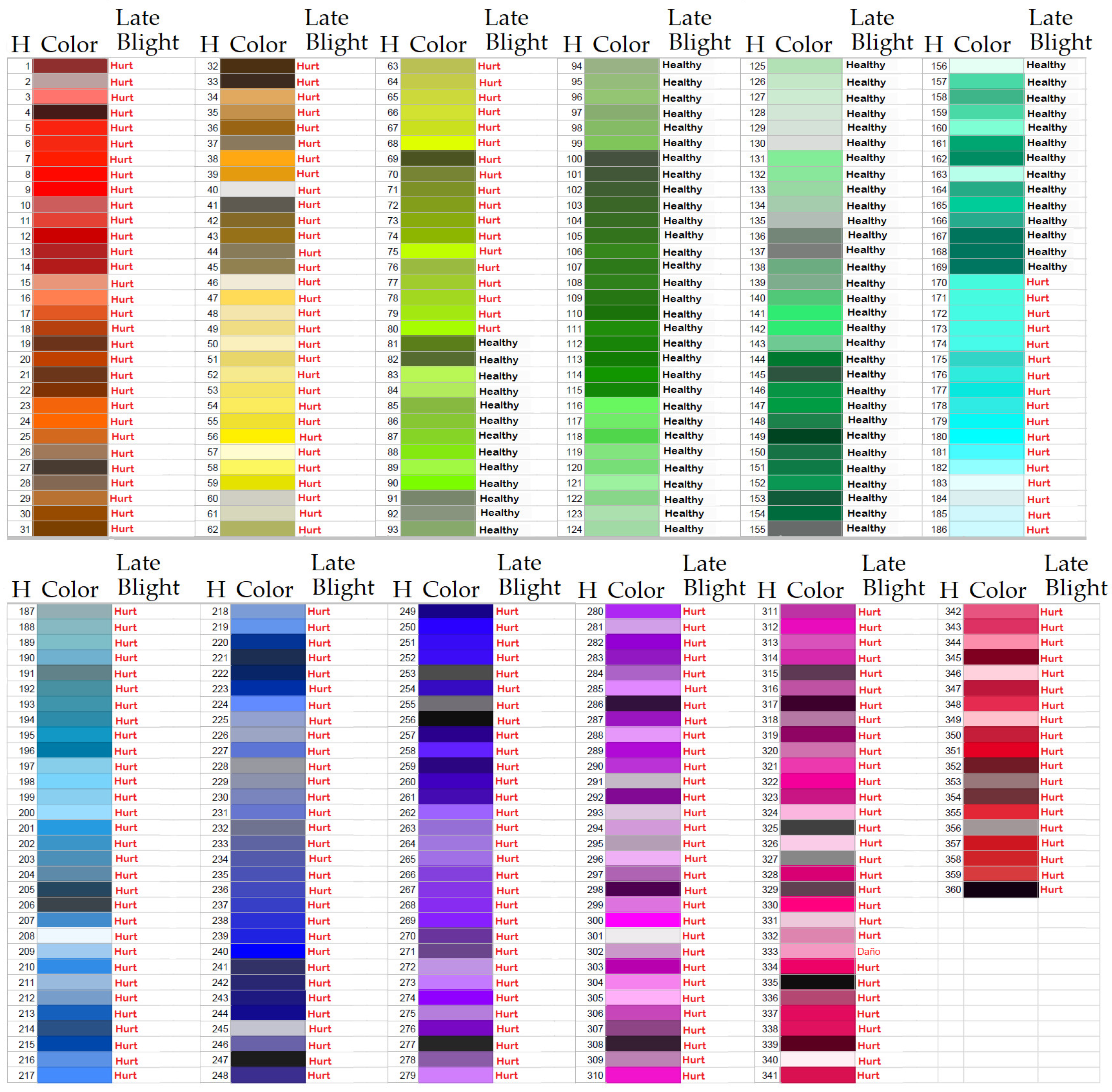
• Segmentation: First, the RGB model was used, and by means of the average of the three channels R, G and B, it was converted to gray scale, then the negative of the image was obtained and on it, immediately, a median filter was applied of a 3×3 mask. Then, it was thresholded by the Otsu method to obtain the optimal binarization threshold, the image was binarized and the related components of the negative of the threshold image by means of Otsu were calculated. The related components of greater area were eliminated and those related components that were not delimited by an area of black pixels where obtained by the binarization by means of Otsu. In this way, the area of the segmented leaf was obtained. Once the color leaf was segmented, the HSV color model was considered, and on the HSV model it was segmented by threshold on the H component, considering the color thresholds in which a plant is damaged by any of the diseases considered, or is healthy. These threshold values were validated by experts in the area of phytopathology. For the case of late blight, Figure 4 shows the color threshold.
• Features extraction: Four color moments for each RGB component and nine statistical measurements were used for texture analysis by GLCM, obtaining a total of 21 features.
• Classification: MLP, K-NN and SVM classifiers were used, using the architecture proposed in Figure 6, i.e., all three classifiers were considered to decide on the output of the classification.

  Table 1. Arguments of the classifiers that make up the proposed architecture.

  Sorter	Accuracy	Arguments
  MLP	healthy-sick	1 hidden layer
  SVM	healthy-sick	kernel linear
  K-NN	healthy-sick	k = 9
  MLP	type-disease	2 hidden layers
  SVM	type-disease	kernel rbf
  K-NN	type-disease	k = 3

  shows the arguments considered for each of the classifiers that were used for the proposed methodology.

Table 2. Sorting results of healthy and sick tomato leaves.

Sorter	Accuracy	—
J48	77.70%	-
KStar	77.29%	-
Random Tree	74.79%	-
LWL	61.45%	-
Decision Stump	61.04%	-
Naive Bayes Updateable	61.16%	-
PART	76.45%	-
Decision Table	74.37%	RMSE
MLP	89.02%	2 hidden layers
SVM	89.03%	Kernel linear
K-NN	85.39%	k = 3
K-NN	83.01%	k = 5
K-NN	70.84%	k = 9
Proposed	86.45%	-

shows the accuracy obtained for the proposed method in which healthy and sick tomato leaves are classified, and in

Table 3. Lesion type classification results: late blight, tomato mosaic virus and Septoria leaf spot.

Sorter	Accuracy	—
J48	92.91%	-
KStar	92.91%	-
Random Tree	90.93%	-
LWL	78.75%	-
Decision Stump	77.5%	-
Naive Bayes Updateable	78.33%	-
PART	91.45%	-
Decision Table	90.72%	RMSE
MLP	98.05%	1 hidden layer
SVM	97.52%	Kernel linear
SVM	97.27%	Kernel rbf
K-NN	94.92%	k = 1
K-NN	93.09%	k = 3
K-NN	95.05%	k = 9
Proposed	97.39%	-

the accuracy obtained in which the type of disease the lesion presented belongs to is classified. The respective tables show the comparison with other models, for which the WEKA platform was used and validated by means of cross validation with $k=10$.

Table 4. Results obtained by other authors.

Architecture	Accuracy	Refs
K-mean	93.63%	[15]
ResNet	97.28%	[19]
SVM	93.75%	[20]
ELM	71.8%	[36]
Inception V3	88%	[37]
CNN	93%	[38]
SqueezeNet	94.93%	[39]
ResNet50	85.98%	[40]
VGG16	90.4%	[41]

shows the accuracy obtained by other authors using different architectures; in each of them, the classes to be classified are healthy class and types of diseases.

5. Discussion

The development of computer systems to support the diagnosis of plant diseases has been of great importance to the agricultural sector in making decisions to act correctly and in time to pests or viruses present. The methodology proposed in this work allows the detection of diseases in tomato leaves.

The methodology is divided into three modules: segmentation, extraction of characteristics and classification. Related works [13] carry out the segmentation of diseases in leaves in a manual way. In the proposed methodology, the segmentation is carried out in an automated way by means of methods in the spatial domain; in addition, the RGB to HSV color model is used for the identification of lesions in the leaves by means of identification from a range of colors that were validated by experts in the area of phytopathology for each of the diseases. Some works [21,28] use color moments in the CIE XYZ color space for feature extraction, while others [36] use eight statistical features based on texture analysis using GLCM. In the proposed methodology, four color moments using the RGB color space and nine statistical measurements using GLCM are used. For the classification module, a decision rule is used to obtain the output corresponding to an input image from the classification obtained by the MLP, K-NN and SVM algorithms in such a way that if two classifiers return the same output, then this will be the final result.

The methodology was applied to the classification of tomato leaves, separating them into diseased and healthy leaves. Later, diseased leaves were classified into three types of diseases: late blight, mosaic virus and Septoria leaf spot. Many works have reported different results in the accuracy values obtained when applying them to detect diseases in leaves; however, in each of them, they consider the healthy class as one more class within the set of classes of diseased leaves to be classified. Ref [36] reported 71.8% using ELM models for late blight detection, another work [37] managed to obtain an accuracy of 88% using the Inception-V3 model, while different authors [38] developed a CNN model with which they achieved an accuracy of 93%. Another study [39] showed that the SqueezeNet model is a good candidate for detecting plant diseases in tomato leaves in a mobile device, obtaining an accuracy of 94.93%. On the other hand, with the proposed model, an accuracy of 86.45% was obtained in the classification of diseased leaves and healthy leaves, while in the classification of the type of disease an accuracy of 97.39% was obtained. The model was compared with other algorithms using the WEKA platform. The results are shown in Table 2 and Table 3.

From the results obtained, it is inferred that the proposed methodology is recommended when you want to classify between different types of diseases present in plant leaves, since the results obtained are competitive to those shown by other authors; however, when it comes to distinguishing between healthy and diseased leaves, other techniques are required that allow you to increase the accuracy compared to the values provided by the WEKA platform. On the other hand, one of the main contributions of this work is to carry out the segmentation process by thresholding using the HSV color model through values registered by an expert in the area of phytopathology, and to make the proposal to use three classifiers in parallel for decision making.

6. Conclusions and Future Work

In this work, a methodology is presented that allows discrimination between images of healthy and sick tomato leaves. In case the leaf is diseased, it is detected which type of disease it suffers from, among late blight, mosaic virus and Septoria leaf spot. The methodology is divided into three modules: (i) segmentation, (ii) extraction of characteristics and (iii) classification. For the segmentation, it is proposed to use thresholding, making use of the HSV color model through a range of colors of the pixels that represent healthy and diseased areas in tomato leaves, validated by an expert in the area of phytopathology. Subsequently, a vector of characteristics corresponding to four color moments for each component of the RGB color model and nine statistical measurements for the texture analysis is constructed using GLCM. Finally, for the classification, an architecture is proposed in which three classifiers are used in parallel (MLP, K-NN and SVM) for decision making through a decision rule that suggests that if two classifiers give the same result, then this will be the end result. The model was validated using k-fold cross validation with k = 10, and it was compared with other models using the WEKA Platform and through the work carried out by other authors via the accuracy presented by the classifiers. The proposed model performs two classifications: firstly, it classifies between classes of diseased leaves and healthy leaves, and secondly, if a leaf is diseased, it detects which type of disease it has, among three to consider (late blight, Septoria leaf spot and mosaic virus).

The proposed methodology obtained an accuracy of 86.45% when classifying healthy tomato leaves with diseased tomato leaves, and an accuracy of 97.39% when classifying the type of disease suffered by a diseased leaf. The results obtained show that the proposed model is adequate compared to other authors when the type of disease is detected; however, when distinguishing between healthy and diseased leaves, it is necessary to analyze other techniques that allow increased accuracy.

The proposed work allows us to obtain a methodology to detect diseases in tomato leaves that can be of support to farmers who are initiated in the study of phytopathology. In the future, machine learning techniques will help improve agricultural productivity in the growth of different crops. In addition, these learning techniques will be implemented in hardware through the use of FPGAs [42,43,44], Arduino [45,46] or in mobile devices [47,48], relying on the use of drones [49,50] for technical monitoring and cultivation tests in order to avoid significant losses in the agricultural sector.

References

1. Organización de las Naciones Unidas para la Alimentación y la Agricultura. Food and Agriculture Organization of the United Nations. Available online: http://www.fao.org/home/es/ (accessed on 24 April 2021).
2. Fideicomisos Instituidos en Relación con la Agricultura. Available online: https://www.fira.gob.mx/ (accessed on 24 April 2021).
3. Li, Y.; Wang, H.; Dang, L.M.; Sadeghi-Niaraki, A.; Moon, H. Crop pest recognition in natural scenes using convolutional neural networks. Comput. Electron. Agric. 2020, 169, 105174. [Google Scholar] [CrossRef]
4. Arsenovic, M.; Karanovic, M.; Sladojevic, S.; Anderla, A.; Stefanovic, D. Solving Current Limitations of Deep Learning Based Approaches for Plant Disease Detection. Symmetry 2019, 11, 939. [Google Scholar] [CrossRef] [Green Version]
5. Atila, Ü.; Uçar, M.; Akyol, K.; Uçar, E. Plant leaf disease classification using EfficientNet deep learning model. Ecol. Informatics 2021, 61, 101182. [Google Scholar] [CrossRef]
6. Nazki, H.; Yoon, S.; Fuentes, A.; Park, D.S. Unsupervised image translation using adversarial networks for improved plant disease recognition. Comput. Electron. Agric. 2020, 168, 105117. [Google Scholar] [CrossRef]
7. Kumbar, B.; Mahmood, R.; Nagesha, S.; Nagaraja, M.; Prashant, D.; Kerima, O.Z.; Karosiya, A.; Chavan, M. Field application of Bacillus subtilis isolates for controlling late blight disease of potato caused by Phytophthora infestans. Biocatal. Agric. Biotechnol. 2019, 22, 101366. [Google Scholar] [CrossRef]
8. Charalampopoulos, I.; Droulia, F. The Agro-Meteorological Caused Famines as an Evolutionary Factor in the Formation of Civilisation and History: Representative Cases in Europe. Climate 2020, 9, 5. [Google Scholar] [CrossRef]
9. Xu, Y.; Zhang, S.; Shen, J.; Wu, Z.; Du, Z.; Gao, F. The phylogeographic history of tomato mosaic virus in Eurasia. Virology 2021, 554, 42–47. [Google Scholar] [CrossRef]
10. Klap, C.; Luria, N.; Smith, E.; Bakelman, E.; Belausov, E.; Laskar, O.; Lachman, O.; Gal-On, A.; Dombrovsky, A. The Potential Risk of Plant-Virus Disease Initiation by Infected Tomatoes. Plants 2020, 9, 623. [Google Scholar] [CrossRef]
11. Ávila, M.C.R.; Lourenço, V.; Quezado-Duval, A.M.; Becker, W.F.; De Abreu-Tarazi, M.F.; Borges, L.C.; Nascimento, A.D.R. Field validation of TOMCAST modified to manage Septoria leaf spot on tomato in the central-west region of Brazil. Crop. Prot. 2020, 138, 105333. [Google Scholar] [CrossRef]
12. Mulugeta, T.; Miuhinyuza, J.B.; Gouws-Meyer, R.; Matsaunyane, L.; Andreasson, E.; Alexandersson, E. Botanicals and plant stregtheners for potato and tomato cultivation in Africa. J. Integr. Agric. 2020, 19, 406–427. [Google Scholar] [CrossRef]
13. Arnal, J.G. Plant disease identification from individual lesions and spots using deep learning. Biosyst. Eng. 2019, 180, 96–107. [Google Scholar] [CrossRef]
14. Saleem, M.H.; Potgieter, J.; Arif, K.M. Plant Disease Detection and Classification by Deep Learning. Plants 2019, 8, 468. [Google Scholar] [CrossRef] [PubMed] [Green Version]
15. Singh, V.; Misra, A. Detection of plant leaf diseases using image segmentation and soft computing techniques. Inf. Process. Agric. 2017, 4, 41–49. [Google Scholar] [CrossRef] [Green Version]
16. Vianna, G.K.; Cunha, G.V.; Oliveira, G.S. A Neural Network Classifier for Estimation of the Degree of Infestation by Late Blight on Tomato Leaves. Int. J. Comput. Inf. Eng. 2017, 11, 18–24. [Google Scholar]
17. Sabrol, H.; Kumar, S. Recognition of Tomato Late Blight by using DWT and Component Analysis. Int. J. Electr. Comput. Eng. 2017, 7, 194–199. [Google Scholar] [CrossRef] [Green Version]
18. Mattos, A.P.; Tolentino, J.B.; Itako, A.T. Determination of the severity of Septoria leaf spot in tomato by using digital im-ages. Australas. Plant Pathol. 2020, 49, 329–356. [Google Scholar] [CrossRef]
19. Zhang, K.; Wu, Q.; Liu, A.; Meng, X. Can Deep Learning Identify Tomato Leaf Disease? Adv. Multimedia 2018, 2018, 1–10. [Google Scholar] [CrossRef] [Green Version]
20. Vetal, S.; Khule, R.S. Tomato plant disease detection using image processing. Int. J. Adv. Res. Comput. Commun. Eng. 2017, 6, 293–297. [Google Scholar] [CrossRef]
21. Sabrol, H.; Satish, K. Tomato plant disease classification in digital images using classification tree. In Proceedings of the IEEE 2016 International Conference on Communication and Signal Processing (ICCSP), Melmaruvathur, India, 6–8 April 2016; pp. 1242–1246. [Google Scholar]
22. Saleem, G.; Akhtar, M.; Ahmed, N.; Qureshi, W. Automated analysis of visual leaf shape features for plant classification. Comput. Electron. Agric. 2019, 157, 270–280. [Google Scholar] [CrossRef]
23. Din, M.Z.; Adnan, S.M.; Ahmad, W.; Aziz, S.; Rashid, J.; Ismail, W.; Iqba, M.J. Classification of Disease in Tomato Plants’ Leaf Using Image Segmentation and SVM. Tech. J. Univ. Eng. Technol. 2018, 23, 81–88. [Google Scholar]
24. Khan, S.; Saboo, M.H.; Narvekar, M.; Sanghvi, D.J. Novel fusion of color balancing and Superpixel based approach for detection of Tomato plant diseases in natural complex environment. J. King Saud Univ. Comput. Inf. Sci. 2020, 1319–1578. [Google Scholar] [CrossRef]
25. Saeed, F.; Khan, M.A.; Sharif, M.; Mittal, M.; Goyal, L.M.; Roy, S. Deep neural network features fusion and selection based on PLS regression with an application for crops diseases classification. Appl. Soft Comput. 2021, 103, 107164. [Google Scholar] [CrossRef]
26. Kumar, S.D.; Esakkirajan, S.; Bama, S.; Keerthiveena, B. A microcontroller based machine vision approach for tomato grading and sorting using SVM classifier. Microprocess. Microsyst. 2020, 76, 103090. [Google Scholar] [CrossRef]
27. Tian, K.; Li, J.; Zeng, J.; Evans, A.; Zhang, L. Segmentation of tomato leaf images based on adaptive clustering number of K-means algorithm. Comput. Electron. Agric. 2019, 165, 104962. [Google Scholar] [CrossRef]
28. Sabrol, H.; Kumar, S. Fuzzy and Neural Network based Tomato Plant Disease Classification using Natural Outdoor Images. Indian J. Sci. Technol. 2016, 9, 1–8. [Google Scholar] [CrossRef]
29. Petrellis, N. Plant Disease Diagnosis for Smart Phone Applications with Extensible Set of Diseases. Appl. Sci. 2019, 9, 1952. [Google Scholar] [CrossRef] [Green Version]
30. Wu, X.; Sun, C.; Zou, T.; Li, L.; Wang, L.; Liu, H. SVM-based image partitioning for vision recognition of AVG guide paths under complex illumination conditions. Robot. Comput. Integr. Manuf. 2020, 61, 101856. [Google Scholar] [CrossRef]
31. Hosseini, S.; Zade, B.M.H. New hybrid method for attack detection using combination of evolutionary algorithms, SVM, and ANN. Comput. Netw. 2020, 173, 107168. [Google Scholar] [CrossRef]
32. Saadatfar, H.; Khosravi, S.; Joloudari, J.H.; Mosavi, A.; Shamshirband, S. A New K-Nearest Neighbors Classifier for Big Data Based on Efficient Data Pruning. Mathematics 2020, 8, 286. [Google Scholar] [CrossRef] [Green Version]
33. Hu, Y.-C. Multilayer Perceptron for Robust Nonlinear Interval Regression Analysis Using Genetic Algorithms. Sci. World J. 2014, 2014, 1–8. [Google Scholar] [CrossRef]
34. Mohanty, S.P.; Hughes, D.P.; Salathé, M. Using Deep Learning for Image-Based Plant Disease Detection. Front. Plant Sci. 2016, 7, 1419. [Google Scholar] [CrossRef] [PubMed] [Green Version]
35. Hughes, D.P.; Salathé, M. An open access repository of images on plant health to enable the development of mobile disease diagnostics through machine learning and crowdsourcing. arXiv 2015, arXiv:1511.08060. [Google Scholar]
36. Xie, C.; Shao, Y.; Li, X.; He, Y. Detection of early blight and late blight diseases on tomato leaves using hyperspectral imaging. Sci. Rep. 2015, 5, 16564. [Google Scholar] [CrossRef] [PubMed]
37. Wan, H.; Lu, Z.; Qi, W.; Chen, Y. Plant Disease Classification Using Deep Learning Methods. In Proceedings of the 4th International Conference on Machine Learning and Soft Computing, ACM, Haiphong City, Vietnam, 17–19 January 2020; pp. 5–9. [Google Scholar]
38. Sharma, P.; Berwal, Y.P.S.; Ghai, W. KrishiMitr (Farmer’s Friend): Using Machine Learning to Identify Diseases in Plants. In Proceedings of the IEEE International Conference on Internet of Things and Intelligence System (IOTAIS), Bali, Indonesia, 1–3 November 2018; pp. 29–34. [Google Scholar]
39. Durmus, H.; Gunes, E.O.; Kirci, M. Disease detection on the leaves of the tomato plants by using deep learning. In Proceedings of the IEEE 2017 6th International Conference on Agro-Geoinformatics, Fairfax, VA, USA, 7–10 August 2017; pp. 1–5. [Google Scholar]
40. Fuentes, A.; Yoon, S.; Kim, S.C.; Park, D.S. A Robust Deep-Learning-Based Detector for Real-Time Tomato Plant Diseases and Pests Recognition. Sensors 2017, 17, 2022. [Google Scholar] [CrossRef] [PubMed] [Green Version]
41. Wang, G.; Sun, Y.; Wang, J. Automatic Image-Based Plant Disease Severity Estimation Using Deep Learning. Comput. Intell. Neurosci. 2017, 2017, 1–8. [Google Scholar] [CrossRef] [Green Version]
42. Prabakaran, G.; Vaithiyanathan, D.; Ganesan, M. FPGA based effective agriculture productivity prediction system using fuzzy support vector machine. Math. Comput. Simul. 2021, 185, 1–16. [Google Scholar] [CrossRef]
43. Yin, L.; Zhang, Y. Village precision poverty alleviation and smart agriculture based on FPGA and machine learning. Microprocess. Microsyst. 2020, 103469. [Google Scholar] [CrossRef]
44. Huang, C.-H.; Chen, P.-J.; Lin, Y.-J.; Chen, B.-W.; Zheng, J.-X. A robot-based intelligent management design for agricultural cyber-physical systems. Comput. Electron. Agric. 2021, 181, 105967. [Google Scholar] [CrossRef]
45. Rodríguez-Robles, J.; Martin, Á.; Martin, S.; Ruipérez-Valiente, J.; Castro, M. Autonomous Sensor Network for Rural Agriculture Environments, Low Cost, and Energy Self-Charge. Sustainability 2020, 12, 5913. [Google Scholar] [CrossRef]
46. Zervopoulos, A.; Tsipis, A.; Alvanou, A.G.; Bezas, K.; Papamichail, A.; Vergis, S.; Stylidou, A.; Tsoumanis, G.; Komianos, V.; Koufoudakis, G.; et al. Wireless Sensor Network Synchronization for Precision Agriculture Applications. Agriculture 2020, 10, 89. [Google Scholar] [CrossRef] [Green Version]
47. Karar, M.E.; Alsunaydi, F.; Albusaymi, S.; Alotaibi, S. A new mobile application of agricultural pests recognition using deep learning in cloud computing system. Alex. Eng. J. 2021, 60, 4423–4432. [Google Scholar] [CrossRef]
48. Hyun, S.; Yang, S.M.; Kim, J.; Kim, K.S.; Shin, J.H.; Lee, S.M.; Lee, B.-W.; Beresford, R.M.; Fleisher, D.H. Development of a mobile computing framework to aid decision-making on organic fertilizer management using a crop growth model. Comput. Electron. Agric. 2021, 181, 105936. [Google Scholar] [CrossRef]
49. Cicioğlu, M.; Çalhan, A. Smart agriculture with internet of things in cornfields. Comput. Electr. Eng. 2021, 90, 106982. [Google Scholar] [CrossRef]
50. Merwe, D.; Burchfield, D.R.; Witt, T.D.; Price, K.P.; Sharda, A. Chapter One—Drones in agriculture. Adv. Agron. 2020, 162, 1–30. [Google Scholar]
Figure 1. Image acquisition.
Electronics 10 01055 g001
Figure 2. Color models: (a) RGB model; (b) HSV model.
Electronics 10 01055 g002
Figure 3. Steps to obtain the segmented image of the leaf.
Electronics 10 01055 g003
Figure 4. Segmentation of the sheet: in (a) original image, (b) gray scale, (c) negative, (d) median filter, (e) method of Otsu, (f) related components, (g) components removed, (h) binarized segmented sheet and (i) segmented color sheet.
Electronics 10 01055 g004
Figure 5. Color range of pixels representing healthy and diseased areas on a late blight leaf (hue component).
Electronics 10 01055 g005
Figure 6. Segmentation of lesion on a tomato leaf infected by Late Blight.
Electronics 10 01055 g006
Figure 7. Architecture of the proposed model.
Electronics 10 01055 g007