A Neuron Model with Dendrite Morphology for Classification

Abstract

Recent neurological studies have shown the importance of dendrites in neural computation. In this paper, a neuron model with dendrite morphology, called the logic dendritic neuron model (LDNM), is proposed for classification. This model consists of four layers: a synaptic layer, a dendritic layer, a membrane layer, and a soma body. After training, the LDNM is simplified by proprietary pruning mechanisms and is further transformed into a logic circuit classifier. Moreover, to address the high-dimensional challenge, feature selection is employed as the dimension reduction method before training the LDNM. In addition, the effort of employing a heuristic optimization algorithm as the learning method is also undertaken to speed up the convergence. Finally, the performance of the proposed model is assessed by five benchmark high-dimensional classification problems. In comparison with the other six classical classifiers, LDNM achieves the best classification performance on two (out of five) classification problems. The experimental results demonstrate the effectiveness of the proposed model. A new perspective for solving classification problems by the proposed LDNM is provided in the paper.

1. Introduction

Biological neural networks are complex and are composed of a large number of interconnected neurons. A neuron is an electrically excitable cell and consists of three typical parts, including a soma (cell body), dendrites, and an axon. Dendrites are filamentous and branch multiple times, constituting the dendritic tree of a neuron. An axon is a slender projection of a neuron. In general, a neuron receives signals via the synapses, which are located on its dendritic tree. Then, the neuron sends out processed signals down its axon. Inspired by the biological neuron model, McCulloch and Pitts first mathematically proposed an artificial neuron model in 1943 [1]. This model worked as a linear threshold gate by comparing a predefined threshold with the sum of inputs that were multiplied by a set of weights. Later, Rosenblatt optimized the artificial neuron model and developed the first perceptron [2]. However, these models are considered to be simplistic and lack flexible computational features. Specifically, nonlinear mechanisms of dendrites were not involved in these models [3].

Koch, Poggio, and Torre are the pioneers who investigated the nonlinear mechanisms of dendrites. They proposed a dendritic neuron model called $\delta$ cell in [4,5]. This model was based on the nonlinear interactions between excitation and inhibition on a dendritic branch. Further studies [6,7,8] also made researchers aware of the importance of dendrites in neural computation. Subsequently, numerous neuron models based on dendritic computation were proposed. For example, Rhodes et al. proposed a model with apical dendrites to reproduce different neuronal firing patterns [9]. Poirazi et al. proposed a neural network model with a nonlinear operation on dendrites [10]. Todo et al. enhanced the nonlinear interaction on the dendrites of a neuron model to simulate directionally selective cells [11]. These works all strengthened the necessity of incorporating mechanisms of dendrites into neural computation.

A classification problem refers to the task where similar objects are grouped into the same classes according to their attributes. Owing to the distinguishing learning capability of artificial neural networks (ANNs), they have been regarded as an alternative classification model for various classification problems, such as credit risk evaluation [12], human recognition [13,14], electroencephalography analysis [15], and disease diagnostics [16]. Although ANNs have shown their high performance for solving classification problems, some issues remain challenging in the application of ANNs. For example, an ANN is not considered as an interpretable model [17]. A determined ANN provides us with little insight into how the classification results are concluded [18]. In addition, as the number of dimensions of a classification problem increases, the size of the ANN grows sharply. Consequently, the training process becomes difficult, and the classification process becomes more time-consuming.

The performance of an ANN is characterized by its learning methods [19]. Backpropagation (BP) algorithms [20,21,22] are commonly used to train ANNs. These BP algorithms utilize the gradient information of the loss function and adjust the weights of neurons in the negative gradient direction. However, the BP algorithms and their variations suffer from two main disadvantages. First, since BP algorithms are the gradient descent algorithms, they are highly sensitive to the initial conditions of an ANN. In other words, BP algorithms may not always find a solution and easily become trapped in local minima [23]. Second, it is not easy to set the learning rate for fast and stable learning. An unsuitable value results in slow convergence or divergence [24]. On the other hand, recent studies have shown that heuristic optimization methods are considered to perform well in the training of ANNs because ANNs are natively suitable for global optimization [25]. These training methods based on heuristic optimization include particle swarm optimization (PSO) [26], the genetic algorithm (GA) [27], the biogeography-based optimizer (BBO) [28], and differential evolution (DE) [29].

In recent years, the use of an artificial neuron model to resolve practical problems has aroused the interest of many researchers. For example, Arec et al. proposed a dendrite morphological neural network with an efficient training algorithm for some synthetic problems and a real-life problem [30]. Hernandez-Barragan et al. proposed an adaptive single-neuron proportional–integral–derivative controller to manipulate a four-wheeled omnidirectional mobile robot [31]. Luo et al. proposed a decision-tree-initialized dendritic neuron model for fast and accurate data classification [32]. In our previous works, various neuron models involved with dendritic computation have been proposed to tackle several real-world issues, such as classification [33,34], function approximation [35], financial time series prediction [36], liver disorder diagnosis [37], tourism demand forecasting [38], and credit risk evaluation [39]. These applications demonstrated the advantages of the dendritic neuron models in solving complicated problems. However, it should be pointed out that the sizes of these proposed neuron models are not very large because the corresponding problems are small-scale applications. Applying dendritic neuron models to large-scale problems has not yet been explored. This prompts us to verify whether a dendritic neuron model can be applied to solve high-dimensional classification problems. On the other hand, with the trend of big data [40,41], not only the dimension but also the number of instances of classification problems becomes increasingly large. As a result, the classification speed of a classifier has drawn the attention of researchers [42,43]. Importantly, we also focus on this aspect when applying dendritic neuron models to high-dimensional classification problems.

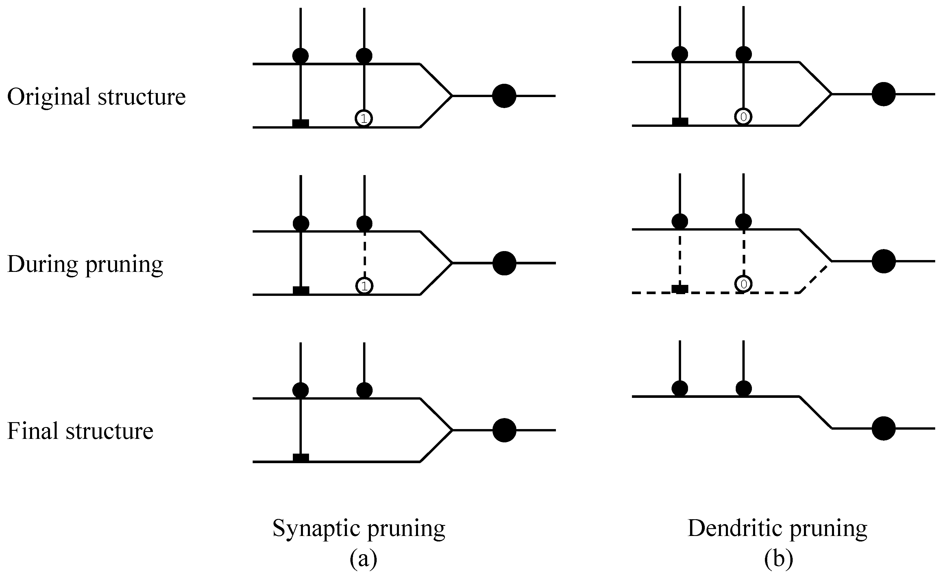
In this study, a neuron model with dendrite morphology called LDNM is proposed to solve high-dimensional classification problems. This neuron model contains four layers: a synaptic layer, a dendritic layer, a membrane layer, and a soma body. The LDNM has structural plasticity, and a trained LDNM can be simplified by means of synaptic pruning and dendritic pruning. It is worth emphasizing that a simplified LDNM can be further transformed into a logic circuit classifier (LCC), which only consists of digital components: comparator, NOT, AND, and OR gates. Compared to most conventional classification methods [44], the proposed LDNM has two novel features. First, for a specific classification problem, the architecture of the trained LDNM can give us some insights into how the classification results are concluded. Second, the trained LDNM can be transformed into an LCC. The classification speed of the LCC is greatly improved when it is implemented in hardware because it only consists of digital components. On the other hand, since the size of the LDNM is considered large when it is applied in high-dimensional classification problems, a heuristic optimization algorithm instead of a BP algorithm is employed in training the LDNM. In addition, feature selection is employed as the dimension reduction method to address the high-dimensional challenge. Finally, five high-dimensional benchmark classification problems are used to evaluate the performance of the proposed model. The experimental results evidence the high performance of LDNM as a very competitive classifier.

The remainder of this paper is organized as follows. The characteristics of the proposed LDNM are described in Section 2. Section 3 presents the two training methods. The experimental studies are provided in Section 4. Finally, Section 5 presents the conclusions of this paper.

2. Proposed Model

2.1. Logic Dendritic Neuron Model

Previous neurological studies strengthened the opinion that the computation performed by dendrites is an indispensable part of neural computation [7,8]. Specifically, the issue regarding the mechanism of dendritic construction was investigated by Koch et al. in their spearheading works [5]. They suggested that the interactions between excitation and inhibition in synapses are nonlinear. An excitation is vetoed by a shunting inhibition that is on the pathway between the excitation and the soma. In other words, logic operations exist on the branch. Furthermore, the interaction between two synaptic inputs is considered a logic AND operation, and the branching points execute a logic OR operation.

Inspired by the abovementioned dendritic mechanism, we propose an LDNM which has a dendrite morphology in this study. The logic architecture of this model is displayed in Figure 1. Four layers compose the LDNM, including a synaptic layer, a dendrite layer, a membrane layer, and a soma body. In detail, the synaptic layers receive and process the input signals that originate in the axons of other neurons. Then, the AND operation is performed on each branch in the dendrite layer. Next, branching points execute the logic OR operation in the membrane layer. Finally, the soma body processes the output of the membrane layer and sends the output signal to its axon. The proposed LDNM can be described mathematically as follows.

2.1.1. Synaptic Layer

The synaptic layer represents the connection where nerve signals are transmitted from a presynaptic neuron to a postsynaptic neuron. A sigmoid function is used to model the synaptic connection in a dendritic branch. The synaptic layer connecting the ith ($i=1,2,...,n$) synaptic input to the jth ($j=1,2,...,m$) dendritic branch is expressed as follows:

$$Y_{ij}=\frac{1}{1+e^{-k(w_{ij}{x}_i-q_{ij})}}$$

(1)

where $x_i$ is the ith synaptic input and ranges in $[0, 1]$. k is a positive constant and is set to 5. $w_{ij}$ and $q_{ij}$ are synaptic parameters that need to be adjusted.

2.1.2. Dendritic Layer

Previous works [45] have shown the existence of multiplicative operations in neurons to process neural information. This idea is also adopted in the proposed model. The dendritic layer performs multiplication to imitate the interaction among synaptic signals on a dendritic branch. This operation is equal to the logic AND operation when the synaptic inputs are binary. The output of the jth dendritic branch $Z_j$ is calculated as follows:

$$Z_j=\prod _{i=1}^n{Y}_{ij}$$

(2)

2.1.3. Membrane Layer

The membrane layer performs the sublinear summation operation on the result collected from all dendritic branches. This operation approximates a logical OR operation in the binary case. The output of the membrane layer V is defined as follows:

$$V=\sum _{j=1}^m{Z}_j$$

(3)

2.1.4. Soma Body

Finally, the output signal of the membrane layer is sent to the soma body. The soma body generates a value of 1 when the input exceeds a specific threshold, and 0 otherwise. A sigmoid function is employed in this layer as follows:

$$O=\frac{1}{1+e^{-k(V-\gamma )}}$$

(4)

where k is a positive constant and is set to 5. The threshold $\gamma$ is set to 0.5 for the classification problem in this study. V is the output of the membrane layer, and O is the output of the soma body.

2.2. Structure Pruning

Structure pruning is an interesting mechanism of many neuron networks [46]. A trained LDNM can also be simplified by proprietary pruning mechanisms. Investigating the synaptic connection described in Equation (1), the states of the synaptic connection can be approximately divided into four types, as shown in Figure 2: constant 1 connection, constant 0 connection, direct connection, and inverse connection. The connection state of a synapse is uniquely determined by its synaptic parameters $w_{ij}$ and $q_{ij}$. Specifically, the threshold ${\theta }_{ij}$ of a synapse is defined as follows:

$${\theta }_{ij}=\frac{q_{ij}}{w_{ij}}$$

(5)

In fact, ${\theta }_{ij}$ describes the position of the image center of the sigmoid function (Equation (1)) on the X-axis, as shown in Figure 2. Four connection states corresponding to six cases are described as follows.

Case 1. 

$w>0$, $q<0<w$, e.g., $w=1$, $q=-0.5$; thus, $\theta =-0.5$, as shown in Figure 2a. This case is a constant 1 connection because the output is always 1, regardless of $x_i$ ranging in $[0, 1]$.

Case 2. 

$w>0$, $0<q<w$, e.g., $w=1$, $q=0.5$; thus, $\theta =0.5$, as shown in Figure 2b. This case is a direct connection because the input with high potential leads to the high output, and vice versa.

Case 3. 

$w>0$, $0<w<q$, e.g., $w=1$, $q=1.5$; thus, $\theta =1.5$, as shown in Figure 2c. This case is a constant 0 connection because the output is always 0, regardless of $x_i$ ranging in [0, 1].

Case 4. 

$w<0$, $w<0<q$, e.g., $w=-1$, $q=0.5$; thus, $\theta =-0.5$, as shown in Figure 2d. This case corresponds to a constant 0 connection.

Case 5. 

$w<0$, $w<q<0$, e.g., $w=-1$, $q=-0.5$; thus, $\theta =0.5$, as shown in Figure 2e. This case is an inverse connection because the input with high potential leads to the low output, and vice versa.

Case 6. 

$w<0$, $q<w<0$, e.g., $w=-1$, $q=-1.5$; thus, $\theta =1.5$, as shown in Figure 2f. This case corresponds to a constant 1 connection.

The values of w and q are all initialized in the range $[-1.5, 1.5]$. Consequently, a synapse is randomly connected to a dendritic branch. After training, the synaptic connection will land on one state of the four connection states, as shown in Figure 3.

Furthermore, owing to the AND logic operation in Equation (2), it is easy to conclude that the constant 1 synaptic connection and the constant 0 synaptic connection play particular roles in the calculation of the output of a branch. More specifically, the constant 1 connection has no influence on the output of a branch. In contrast, the output of a branch is always 0 when a constant 0 synapse is connected to it. Thus, two pruning operations on a trained LDNM can be proposed. Figure 4a shows the synaptic pruning, where a constant 1 synaptic connection is screened out. Figure 4b shows the dendritic pruning, where the dendritic branch connected to a constant 0 is screened out.

2.3. Transforming the LDNM into a Logical Circuit

Similar to multilayer perceptrons (MLPs) [28], the proposed LDNM can also be applied in classification problems [33]. After supervised learning on a dataset, a unique LDNM with adjusted synaptic parameters $w_{ij}$s and $q_{ij}$s is generated. Then, the pruning operations are executed, and a more concise LDNM for the specific classification problem is obtained.

It is worth emphasizing that a determined LDNM can be further transformed into a logic circuit. Figure 5 shows an example of a determined LDNM and its equivalent logic circuit. The synapse connection is equivalent to a comparator coupled with a NOT gate or without it. The dendritic layer is equivalent to an AND gate, the membrane layer is an OR gate, and the soma body can be considered as a wire.

The hallmark of the LDNM as a classifier is that an equivalent logic circuit can be generated from it. Classical classifiers, e.g., k-nearest neighbors (KNN), support vector machine (SVM), and naive Bayes (NB), are based on mathematical analysis and a large amount of floating-point computation. Compared with these classifiers, the LCC has a very high speed because it has no floating-point computation but only contains logic operations. In fact, with the trend of big data [40], the speed of a classifier is becoming more important in practical applications.

3. Learning Methods

Two learning methods are employed and compared in this study. The first one is the BP algorithm. The other method is a heuristic optimization algorithm.

3.1. Backpropagation Algorithm

Since the proposed LDNM is a feed-forward model, the error BP learning rule can be adopted in training the LDNM. Specifically, the error between the ideal output $T_p$ and the actual output $O_p$ of a neuron on the pth training sample is defined as follows:

$$E_p=\frac{1}{2}{(T_p-O_p)}^2$$

(6)

Then, to minimize $E_p$, the synaptic parameters $w_{ij}$ and $q_{ij}$ are corrected in the negative gradient direction as follows:

$$\Delta w_{ij}=-\eta \sum _{p=1}^P\frac{\partial E_p}{\partial w_{ij}}$$

(7)

$$\Delta q_{ij}=-\eta \sum _{p=1}^P\frac{\partial E_p}{\partial q_{ij}}$$

(8)

where $\eta$ is the learning rate, and P is the number of training samples. The synaptic parameters $w_{ij}$ and $q_{ij}$ are updated at the next iteration $t+1$ as follows:

$$w_{ij}(t+1)=w_{ij}\left(t\right)+\Delta w_{ij}$$

(9)

$$q_{ij}(t+1)=q_{ij}\left(t\right)+\Delta q_{ij}$$

(10)

In particular, the partial differentials of $E_p$ with respect to the synaptic parameters $w_{ij}$ and $q_{ij}$ can be calculated as follows:

$$\frac{\partial E_p}{\partial w_{ij}}=\frac{\partial E_p}{\partial O_p}·\frac{\partial O_p}{\partial V}·\frac{\partial V}{\partial Z_j}·\frac{\partial Z_j}{\partial Y_{ij}}·\frac{\partial Y_{ij}}{\partial w_{ij}}$$

(11)

$$\frac{\partial E_p}{\partial q_{ij}}=\frac{\partial E_p}{\partial O_p}·\frac{\partial O_p}{\partial V}·\frac{\partial V}{\partial Z_j}·\frac{\partial Z_j}{\partial Y_{ij}}·\frac{\partial Y_{ij}}{\partial q_{ij}}$$

(12)

The components in Equations (11) and (12) are expressed as follows:

$$\frac{\partial E_p}{\partial O_p}=O_p-T_p$$

(13)

$$\frac{\partial O_p}{\partial V}=\frac{k{e}^{-k(V-\gamma )}}{{(1+e^{-k(V-\gamma )})}^2}$$

(14)

$$\frac{\partial V}{\partial Z_j}=1$$

(15)

$$\frac{\partial Z_j}{\partial Y_{ij}}=\frac{1}{Y_{ij}}\prod _{h=1}^n{Y}_{hj}$$

(16)

$$\frac{\partial Y_{ij}}{\partial w_{ij}}=\frac{k{x}_i{e}^{-k(x_i{w}_{ij}-q_{ij})}}{{(1+e^{-k(x_i{w}_{ij}-q_{ij})})}^2}$$

(17)

$$\frac{\partial Y_{ij}}{\partial q_{ij}}=\frac{-k{e}^{-k(x_i{w}_{ij}-q_{ij})}}{{(1+e^{-k(x_i{w}_{ij}-q_{ij})})}^2}$$

(18)

3.2. Competitive Swarm Optimizer

BP has been proven to be a very effective method to train ANNs [20]. However, the dependence on gradient information makes BP sensitive to the initial condition [23]. In addition, the slow convergence speed and the capability of being easily trapped in local minima are the main disadvantages of BP methods [24]. In contrast, the utility of a heuristic optimization method to solve real-world problems [47,48] has aroused the interest of researchers in recent years, including training ANNs [28,34]. The heuristic optimization algorithm called the competitive swarm optimizer (CSO) is also employed to train the LDNM in this study.

The CSO is a novel evolutionary method for large-scale optimization that was proposed by Chen et al. recently [49]. This algorithm is based on a pairwise competition mechanism and is proven effective for solving practical problems [50,51]. CSO is similar to PSO and works as follows. Each particle in CSO is attributed by two vectors: the position vector $\mathbf{x}$ and the velocity vector $\mathbf{v}$. In contrast to PSO [52], the particle in CSO learns from its competitors rather than its personal best or the global best. In iteration t, the swarm in CSO is divided into two groups randomly, and pairwise competitions are executed immediately. Then, the winner particles are directly passed to the next generation. Meanwhile, the loser particles learn from their corresponding winners and update their positions as follows:

$${\mathbf{v}}_{loser}^{(t+1)}=R_1^{\left(t\right)}{\mathbf{v}}_{loser}^{\left(t\right)}+R_2^{\left(t\right)}({\mathbf{x}}_{winner}^{\left(t\right)}-{\mathbf{x}}_{loser}^{\left(t\right)})+\varphi R_3^{\left(t\right)}({\overline{\mathbf{x}}}^{\left(t\right)}-{\mathbf{x}}_{loser}^{\left(t\right)})$$

(19)

$${\mathbf{x}}_{loser}^{(t+1)}={\mathbf{x}}_{loser}^{\left(t\right)}+{\mathbf{v}}_{loser}^{(t+1)}$$

(20)

where ${\mathbf{x}}_{loser}$ and ${\mathbf{v}}_{loser}$ are the position and velocity of the loser, respectively. ${\mathbf{x}}_{winner}$ is the position of the winner particle. $R_1$, $R_2$, and $R_3$ are three random vectors within [0, 1]. $\varphi$ is the parameter that controls the influence of the mean position of the current swarm $\overline{\mathbf{x}}$. Finally, the main loop of the CSO terminates if the stopping criterion is met.

To employ the CSO as the learning method, all the synaptic parameters ($w_{ij}$s and $q_{ij}$s) of an untrained LDNM are encoded as a vector for optimization. The position vector $\mathbf{x}$ of each particle in CSO represents a candidate solution and can be encoded as follows:

$$\mathbf{x}=(w_{1,1},w_{1,2},...,w_{nm},q_{1,1},q_{1,2},...,q_{nm})$$

(21)

where the definitions of n and m are the same as Equation (23). The fitness function of a particle in CSO, which evaluates an LDNM, is defined as the mean square error (MSE):

$$fitness=\frac{1}{2P}\sum _{p=1}^P{(T_p-O_p)}^2$$

(22)

where the definitions of $O_p$, $T_p$, p, and P are the same as above. During the process of training an LDNM, the CSO iteratively changes all of the $w_{ij}$s and $q_{ij}$s to minimize the value of MSE.

3.3. Feature Selection before Learning

Our previous works have shown the high performance of dendritic neuron models for classification problems [33,37,39]. However, it is not easy to apply a dendritic neuron model to high-dimensional classification problems because of the large number of synaptic parameters. The number of synaptic parameters ($w_{ij}$ and $q_{ij}$) in the proposed LDNM is calculated as follows:

$$N=2\ast n\ast m$$

(23)

where n and m are the number of synaptic inputs and dendritic branches, respectively. Usually, m is set to $2n$. As a result, the complexity of an LDNM increases with the square of the number of synaptic inputs. Thus, dimension reduction is a natural method when applying an LDNM to a high-dimensional classification problem.

In general, dimension reduction methods can be roughly divided into two categories: feature extraction and feature selection [53]. The former methods transform original data from the high-dimensional space into a low-dimensional space. Finally, derived features are obtained. Two typical feature extraction methods are principal component analysis (PCA) and linear discriminant analysis (LDA). On the other hand, feature selection tries to select the most optimal subset of features from the original features. Feature selection rather than feature extraction is employed to perform dimension reduction in this study. Compared with feature extraction methods, feature selection methods are considered more simple and require less computation power. The optimal subset of relevant features selected by a feature selection method can improve the performance of a classifier. In addition, a determined feature selection model has no need of extra calculation. Thus, it can work better with the LDNM in classification tasks.

More features increase the difficulty of training an LDNM. However, more features also mean more information. Therefore, it is a trade-off to determine the number of features after dimension reduction. On the other hand, structure pruning also plays the role of feature selection for a trained LDNM such that irrelevant features are removed by synaptic pruning and dendritic pruning in the final structure, as shown in Figure 4. Such pruning indicates that some irrelevant features are permitted to be retained after feature selection before training an LDNM. In other words, as many features as possible should be retained before training an LDNM because more information is provided.

4. Experimental Studies

This section presents the experiments to evaluate the performance of the proposed LDNM. All algorithms in this study are implemented in C and Python language. The experiments are executed on the Linux 64-bit system with a Core-i5 CPU with 8 G RAM.

4.1. Experimental Setup for Determining the Suitable Learning Method

We use two high-dimensional benchmark classification datasets to verify the characteristics of the proposed model. The two datasets are the Wisconsin diagnostic breast cancer (WDBC) dataset [54] and the Ionosphere dataset [55], which can be accessed via the UCI machine learning repository. WDBC describes the breast cancer diagnosis according to the features that are computed from a digitized image of a fine needle aspirate of a breast mass. The Ionosphere dataset describes the collected radar data to determine whether signals pass through the ionosphere. The two problems are all binary classification problems, and the details of them are summarized in

Table 1. The details of the benchmark datasets.

Dataset	Num. of Samples	Num. of Features	Types of Features	Num. of Classes	Num. of Instances for Each Class
WDBC	569	30	continuous	2	357, 212
Ionosphere	351	34	continuous	2	225, 126

.

Each dataset is randomly separated into two subsets. The training subset is used to train the LDNM, and the testing one is used to validate the model. The proportions of each subset are set to 50%–50%. Specifically, all features (attributes) of each dataset are normalized in the range [0, 1] to fit the input of the proposed LDNM. In addition, the hyper-parameters k and $\gamma$ of LDNM are set to the typical values (5 and 0.5, respectively).

Mutual information (MI) [56] is a metric that measures the dependence of two variables, and a higher MI corresponds to a higher dependency. MI is sensitive to linear dependency and other kinds of dependency between variables. A simple univariate feature selection method based on MI is employed to select the best feature subset before training. The employed feature selection method is considered as a filter [53] and works as follows. First, the MI between each feature and class is computed. Then, the features with the highest values of MI are selected. Specifically, 16 features are selected for each dataset in this study. Consequently, the number of synaptic parameters is approximately limited under 1000. In fact, other effective feature selection methods [53,57] can also be employed in this step.

4.2. The Results Obtained by Four Training Methods

To investigate the influence of feature selection in training LDNMs, four training methods are employed to train LDNMs for the two classification problems. These methods are feature selection plus CSO (FS+CSO), CSO, feature selection plus BP (FS+BP), and BP. Note that only the training data are used to determine the feature subset that will be further used to reduce the dimension of training data and testing data. In addition, to ensure a fair comparison between CSO and BP, the maximum number of evaluations of CSO is set to 20,000, and the maximum number of iterations of BP is set to 10,000. In fact, BP takes more memory and training time than CSO in this setup.

The experiments of each training method are performed 30 times on two benchmark problems independently. The statistical results of MSE, training classification accuracy, and testing classification accuracy are provided in

Table 2. The statistical results of four training methods for two problems.

Dataset	Training Methods	MSE	Training Accuracy (%)	Test Accuracy (%)
WDBC	CSO	3.44$\times {10}^{-2}$ ± 2.57$\times {10}^{-3}$	94.30 ± 0.87	93.47 ± 1.52
	FS+CSO	2.54$\times {10}^{-2}$ ± 2.57$\times {10}^{-3}$	94.69 ± 1.02	94.15± 0.92
	BP	1.60$\times {10}^{-1}$ ± 8.34$\times {10}^{-3}$	62.85 ± 1.97	62.63 ± 1.97
	FS+BP	5.47$\times {10}^{-2}$ ± 5.18$\times {10}^{-2}$	87.06 ± 11.90	86.64 ± 12.38
Ionosphere	CSO	7.61$\times {10}^{-2}$ ± 6.24$\times {10}^{-3}$	82.05 ± 2.52	79.68 ± 3.20
	FS+CSO	4.86$\times {10}^{-2}$ ± 8.66$\times {10}^{-3}$	89.47 ± 2.31	84.46 ± 2.92
	BP	1.54$\times {10}^{-1}$ ± 1.04$\times {10}^{-2}$	64.32 ± 2.44	63.89 ± 2.46
	FS+BP	9.96$\times {10}^{-2}$ ± 3.92$\times {10}^{-2}$	76.44 ± 8.95	74.72 ± 8.69

. In addition, classification accuracy has the following definition:

$$Classificationaccuracy=\frac{Numberofcorrectpredictions}{Totalnumberofpredictions}\ast 100\%$$

(24)

It is obvious that employing feature selection benefits the subsequent training process because the performance of the training methods with feature selection is ultimately improved. Specifically, the testing classification accuracies of the four methods are exhibited in Figure 6. This figure also shows the positive influence of feature selection on the subsequent training process because the testing accuracy is improved assuredly. Although an extra computing cost is introduced in feature selection, fewer features are selected after feature selection, and fewer synaptic parameters of LDNM are produced. Thus, a lower amount of computing resources is ultimately necessary in the subsequent training process. Therefore, not only the classification accuracy but also the training speed is improved by feature selection [53].

Comparing the performance of CSO with BP on training LDNMs, it is clear that CSO outperforms BP because the MSE and testing classification accuracy obtained by CSO are better than those obtained by BP. This result indicates that CSO is more powerful than BP in training an LDNM. Moreover, BP consumes more computational resources in training LDNMs.

To further investigate the differences in the four training methods in training LDNMs, the average (30 times) convergence curves of these methods for two benchmark problems are plotted in Figure 7. These curves reflect the efficiency and stability of a training method. It is clear that feature selection speeds up the convergence because those methods that are coupled with feature selection converge faster than the ones without feature selection. Moreover, BP is easily trapped in a local minimum [23,25] and is even invalid when the size of an LDNM is large. These findings indicate that BP is not an effective learning method for training LDNMs for high-dimensional classification problems.

4.3. Investigating Structure Pruning and Logic Circuit Transformation

As mentioned above, the structure of a trained LDNM can be pruned by synaptic pruning and dendritic pruning. Then, an LCC is obtained, which is transformed from the pruned LDNM. The performance of the pruned LDNM and the LCC is also verified in this section. The FS+CSO combination is employed as the training method and is performed 30 times. The classification accuracy of the pruned LDNMs and the LCCs of the trained LDNMs is verified on the same test data.

Table 3. The comparison of the test classification accuracy among different classifiers for two problems.

Dataset	Test Classification Accuracy (%)
	LDNM	Pruned LDNM	LCC
WDBC	94.15 ± 0.92	93.19 ± 3.11	90.02 ± 3.48
Ionosphere	84.46 ± 2.91	84.38 ± 3.43	85.70 ± 3.45

shows the classification results. It is clear that the performance of the pruned LDNMs and the LCCs has no significant degradation compared with their corresponding LDNMs. This finding indicates the feasibility of this transformation.

Two pruned LDNMs and their corresponding LCCs for the two benchmark problems are shown in Figure 8. In contrast to general ANNs that lack interpretation, the pruned LDNM and its corresponding LCC provide us with some insights into how the classification results are concluded. For example, there are two dendritic branches in the final LDNM for the WDBC problems, as shown in Figure 8a. This observation means that two patterns of the input data determine the classification. In the first pattern, when the 8th, 21st, and 28th input are all larger than the three thresholds, the LDNM outputs 1, and 0 otherwise. The second pattern has a similar explanation. These patterns benefit our understanding of the intrinsic characteristics of these problems.

4.4. Comparison with Classical Classifiers

The above experiments have shown that feature selection plus CSO is the most effective learning method in training LDNM, because this method has the fastest convergence speed and the highest classification accuracy. In this subsection, we also compare LDNM with other classical classifiers to verify the performance of LDNM. These classifiers include KNN, SVM, decision tree, random forest, MLP, and NB. The parameters of the seven classifiers are set as shown in

Table 4. Parameter settings for seven classifiers.

Classifier	Parameter	Setting
LDNM	Positive constant (k)	5
	The threshold in soma body ($\gamma$)	0.5
KNN	Number of neighbors (k)	3
SVM	Kernel	rbf
	Penalty parameter	0.5
Decision tree	Maximum depth of the tree	8
Random forest	Number of trees	5
	Depth of the tree	3
MLP	Number of layers	3
	Number of neurons in hidden layer	100
NB	Assumption of feature distribution	Gaussian

. In addition to the abovementioned two classification problems, the other three benchmark classification datasets are also employed in this experiment. More details about these three datasets are presented in

Table 5. The details of three benchmark datasets.

Dataset	No. of Samples	No. of Features	No. of Classes	No. of Instances for Each Class (0/1)
ForestTypes	325	27	2	189, 136
RAFPD	240	46	2	120, 120
SPECTF	267	44	2	55, 212

.

For each classifier, we conduct three times 10-fold cross-validation (CV) [58] to evaluate its effectiveness. Figure 9 is the box and whisker diagram which shows the classification accuracy of these classifiers on the five benchmark datasets. From Figure 9, we can see that there is no one classifier that always outperforms the others on all of the classification datasets. In addtion, we can see that LDNM has higher medians than most of the remaining classifiers on the datasets ForestTypes, Ionosphere, RAFPD, and SPECTF. It indicates that LDNM has a stronger classification ability in comparison with the others. In addition, the interquartile range (IR) in Figure 9 which is the length between the first and the third quartile reflects stability of classification performance. A shorter IR means a more stable performance. From Figure 9, we can see that LDNM has acceptable solutions with short IR. It indicates that the stability of LDNM is considered competitive in comparison with the other classifiers. The classification accuracy of these classifiers on five benchmark datasets is summarized in

Table 6. The comparisons of the classification accuracy among different classifiers for five problems.

Classifier	Forest Types	Ionosphere	RAFPD	SPECTF	WDBC
KNN	86.57 ± 5.38	85.57 ± 5.53	82.36 ± 5.53	71.20 ± 9.25	96.78 ± 1.57
SVM	83.60 ± 7.96	81.11 ± 5.92	81.25 ± 5.92	79.42 ± 9.27	93.96 ± 2.40
Decision tree	85.03 ± 5.78	87.65 ± 6.28	74.44 ± 6.28	72.45 ± 10.02	92.39 ± 3.18
Random forest	83.90 ± 6.41	88.90 ± 4.69	79.44 ± 4.69	78.80 ± 9.88	94.08 ± 2.99
MLP	84.62 ± 6.51	86.90 ± 6.44	75.97 ± 6.44	79.42 ± 9.27	95.37 ± 2.50
NB	80.92 ± 8.20	88.41 ± 5.71	83.75 ± 5.71	67.72 ± 8.96	93.15 ± 3.08
LDNM	86.66 ± 5.99	87.35 ± 7.04	80.00 ± 7.64	80.53 ± 8.71	94.44 ± 2.44

. From Table 6, we can see that LDNM, KNN, random forest, and NB achieve the best classification performance on two, one, one, and one classification problems, respectively. The comparison result suggests that the proposed LDNM can obtain better or very competitive results with these classifiers in terms of test classification accuracy.

To further determine the significant differences among the classification accuracy of these classifiers, we conduct the Friedman test on the classification accuracy of these classifiers in Table 6.

Table 7. Statistical results obtained by Friedman test on the classification accuracy in Table 6.

Classifier	Ranking	z Value	p Value	${\mathit{p}}_{\mathbf{bonf}}$ Value
LDNM	3.26	-	-	-
KNN	3.6867	1.710472	0.087179	0.523072
MLP	3.8333	2.298447	0.021536	0.129218
Random forest	3.85	2.365262	0.018017	0.108104
NB	4.3367	4.316269	0.000016	0.000095
SVM	4.38	4.489989	0.000007	0.000043
Decision tree	4.6533	5.58576	0	0

presents the statistical results, including the values of ranking, z value, unadjusted p value, and $p_{bonf}$ value. From Table 7, we can see that LDNM obtains the smallest ranking value of 3.26. It means that LDNM achieves the best performance among these classifiers in terms of test classification accuracy. In addition, we investigate the significance among these classifiers. To avoid the Type I error [59], we use a post hoc test, i.e., the Bonferroni–Dunn, to adjust the p values. From Table 7, we can see that the adjusted p values, i.e., $p_{bonf}$ values, of KNN, MLP, and random forest are larger than the significance level ($\alpha$ = 0.05). This indicates that LDNM is not significantly better but obtains competitive results in comparison with the three classifiers. In addition, the $p_{bonf}$ values of NB, SVM, and decision tree are smaller than 0.05. This indicates that LDNM is significantly superior to the three classifiers on the five classification problems. Therefore, we can conclude that the proposed LDNM can be considered as a very competitive classifier in comparison with these state-of-the-art classifiers.

5. Conclusions

Recent research has strongly suggested that dendrites play an important role in neural computation. In this paper, a novel neuron model with dendrite morphology, called the logic dendritic neuron model, was proposed for solving classification problems. This model consists of four layers: a synaptic layer, a dendritic layer, a membrane layer, and a soma body. To apply this model to high-dimensional classification problems, we employed the feature selection method to reduce the dimensionality of the classification problems, although the reduced dimensionality is still comparatively high for the proposed LDNM. In addition, we attempted to use a heuristic optimization algorithm called CSO to train the proposed LDNM. This method was verified to be more suitable than BP in training the LDNM with numerous synaptic parameters. Finally, we compared LDNM with the other six classical classifiers on five classification problems to verify its performance. The comparison result indicated that the proposed LDNM can obtain better or very competitive results with these classifiers in terms of test classification accuracy.

It is worth pointing out that the proposed LDNM has two unique characteristics. First, a trained LDNM can be simplified by synaptic pruning and dendritic pruning. Second, the simplified LDNM can be transformed into a logic circuit classifier for a specific classification problem. It can be expected that the speed achieved by the logic circuit classifier is high when this model is implemented in hardware. In addition, the the trained LDNM provides us with some insights into the specific problem. However, it should be noted that the feature selection method chosen in this study was very simple. Therefore, more effective feature selection methods are required when solving more complicated problems.

In future studies, we will apply the proposed LDNM to more classification tasks to verify its effectiveness. The improvement of the architecture of the dendritic neuron model and the learning methods deserve our unremitting efforts. In addition, extending the proposed LDNM to dealing with multiclass classification problems is worth investigating. Moreover, implementing the proposed LDNM as a module unit in hardware is our future research topic.

References

1. McCulloch, W.S.; Pitts, W. A logical calculus of the ideas immanent in nervous activity. Bull. Math. Biophys. 1943, 5, 115–133. [Google Scholar] [CrossRef]
2. Rosenblatt, F. The perceptron: A probabilistic model for information storage and organization in the brain. Psychol. Rev. 1958, 65, 386. [Google Scholar] [CrossRef] [PubMed] [Green Version]
3. London, M.; Häusser, M. Dendritic computation. Annu. Rev. Neurosci. 2005, 28, 503–532. [Google Scholar] [CrossRef] [Green Version]
4. Koch, C.; Poggio, T.; Torre, V. Retinal ganglion cells: A functional interpretation of dendritic morphology. Phil. Trans. R. Soc. Lond. B 1982, 298, 227–263. [Google Scholar]
5. Koch, C.; Poggio, T.; Torre, V. Nonlinear interactions in a dendritic tree: Localization, timing, and role in information processing. Proc. Natl. Acad. Sci. USA 1983, 80, 2799–2802. [Google Scholar] [CrossRef] [Green Version]
6. Agmon-Snir, H.; Carr, C.E.; Rinzel, J. The role of dendrites in auditory coincidence detection. Nature 1998, 393, 268. [Google Scholar] [CrossRef] [PubMed]
7. Magee, J.C. Dendritic integration of excitatory synaptic input. Nat. Rev. Neurosci. 2000, 1, 181. [Google Scholar] [CrossRef] [PubMed]
8. Euler, T.; Detwiler, P.B.; Denk, W. Directionally selective calcium signals in dendrites of starburst amacrine cells. Nature 2002, 418, 845. [Google Scholar] [CrossRef] [PubMed]
9. Rhodes, P.A.; Llinás, R.R. Apical tuft input efficacy in layer 5 pyramidal cells from rat visual cortex. J. Physiol. 2001, 536, 167–187. [Google Scholar] [CrossRef]
10. Poirazi, P.; Brannon, T.; Mel, B.W. Arithmetic of subthreshold synaptic summation in a model CA1 pyramidal cell. Neuron 2003, 37, 977–987. [Google Scholar] [CrossRef] [Green Version]
11. Todo, Y.; Tamura, H.; Yamashita, K.; Tang, Z. Unsupervised learnable neuron model with nonlinear interaction on dendrites. Neural Netw. 2014, 60, 96–103. [Google Scholar] [CrossRef] [PubMed]
12. Baesens, B.; Setiono, R.; Mues, C.; Vanthienen, J. Using neural network rule extraction and decision tables for credit-risk evaluation. Manag. Sci. 2003, 49, 312–329. [Google Scholar] [CrossRef] [Green Version]
13. Melin, P.; Sánchez, D.; Castillo, O. Genetic optimization of modular neural networks with fuzzy response integration for human recognition. Inf. Sci. 2012, 197, 1–19. [Google Scholar] [CrossRef]
14. Zhao, X.; Chen, Y.; Guo, J.; Zhao, D. A spatial-temporal attention model for human trajectory prediction. IEEE/CAA J. Autom. Sin. 2020, 7, 965–974. [Google Scholar] [CrossRef]
15. Kasabov, N.; Capecci, E. Spiking neural network methodology for modelling, classification and understanding of EEG spatio-temporal data measuring cognitive processes. Inf. Sci. 2015, 294, 565–575. [Google Scholar] [CrossRef]
16. Anthimopoulos, M.; Christodoulidis, S.; Ebner, L.; Christe, A.; Mougiakakou, S. Lung pattern classification for interstitial lung diseases using a deep convolutional neural network. IEEE Trans. Med Imaging 2016, 35, 1207–1216. [Google Scholar] [CrossRef]
17. Olden, J.D.; Jackson, D.A. Illuminating the “black box”: A randomization approach for understanding variable contributions in artificial neural networks. Ecol. Model. 2002, 154, 135–150. [Google Scholar] [CrossRef]
18. Andrews, R.; Diederich, J.; Tickle, A.B. Survey and critique of techniques for extracting rules from trained artificial neural networks. Knowl.-Based Syst. 1995, 8, 373–389. [Google Scholar] [CrossRef]
19. Lippmann, R. An introduction to computing with neural nets. IEEE Assp Mag. 1987, 4, 4–22. [Google Scholar] [CrossRef]
20. Hagan, M.T.; Menhaj, M.B. Training feedforward networks with the Marquardt algorithm. IEEE Trans. Neural Netw. 1994, 5, 989–993. [Google Scholar] [CrossRef]
21. Zhang, N. An online gradient method with momentum for two-layer feedforward neural networks. Appl. Math. Comput. 2009, 212, 488–498. [Google Scholar] [CrossRef]
22. Mall, S.; Chakraverty, S. Single layer Chebyshev neural network model for solving elliptic partial differential equations. Neural Process. Lett. 2017, 45, 825–840. [Google Scholar] [CrossRef]
23. Magoulas, G.; Vrahatis, M.; Androulakis, G. On the alleviation of the problem of local minima in back-propagation. Nonlinear Anal. 1997, 30, 4545–4550. [Google Scholar] [CrossRef]
24. Vogl, T.P.; Mangis, J.; Rigler, A.; Zink, W.; Alkon, D. Accelerating the convergence of the back-propagation method. Biol. Cybern. 1988, 59, 257–263. [Google Scholar] [CrossRef]
25. Zhang, L.; Suganthan, P.N. A survey of randomized algorithms for training neural networks. Inf. Sci. 2016, 364, 146–155. [Google Scholar] [CrossRef]
26. Meissner, M.; Schmuker, M.; Schneider, G. Optimized Particle Swarm Optimization (OPSO) and its application to artificial neural network training. BMC Bioinform. 2006, 7, 125. [Google Scholar] [CrossRef] [Green Version]
27. Ding, S.; Su, C.; Yu, J. An optimizing BP neural network algorithm based on genetic algorithm. Artif. Intell. Rev. 2011, 36, 153–162. [Google Scholar] [CrossRef]
28. Mirjalili, S.; Mirjalili, S.M.; Lewis, A. Let a biogeography-based optimizer train your multi-layer perceptron. Inf. Sci. 2014, 269, 188–209. [Google Scholar] [CrossRef]
29. Wang, L.; Zeng, Y.; Chen, T. Back propagation neural network with adaptive differential evolution algorithm for time series forecasting. Expert Syst. Appl. 2015, 42, 855–863. [Google Scholar] [CrossRef]
30. Arce, F.; Zamora, E.; Sossa, H.; Barrón, R. Differential Evolution Training Algorithm for Dendrite Morphological Neural Networks. Appl. Soft Comput. 2018, 68, 303–313. [Google Scholar] [CrossRef]
31. Hernandez-Barragan, J.; Rios, J.D.; Alanis, A.Y.; Lopez-Franco, C.; Gomez-Avila, J.; Arana-Daniel, N. Adaptive Single Neuron Anti-Windup PID Controller Based on the Extended Kalman Filter Algorithm. Electronics 2020, 9, 636. [Google Scholar] [CrossRef]
32. Luo, X.; Wen, X.; Zhou, M.; Abusorrah, A.; Huang, L. Decision-Tree-Initialized Dendritic Neuron Model for Fast and Accurate Data Classification. IEEE Trans. Neural Netw. Learn. Syst. 2021, 1–11. [Google Scholar] [CrossRef]
33. Ji, J.; Gao, S.; Cheng, J.; Tang, Z.; Todo, Y. An approximate logic neuron model with a dendritic structure. Neurocomputing 2016, 173, 1775–1783. [Google Scholar] [CrossRef]
34. Ji, J.; Song, S.; Tang, Y.; Gao, S.; Tang, Z.; Todo, Y. Approximate logic neuron model trained by states of matter search algorithm. Knowl.-Based Syst. 2019, 163, 120–130. [Google Scholar] [CrossRef]
35. Gao, S.; Zhou, M.; Wang, Y.; Cheng, J.; Yachi, H.; Wang, J. Dendritic neuron model with effective learning algorithms for classification, approximation, and prediction. IEEE Trans. Neural Netw. Learn. Syst. 2018, 30, 601–614. [Google Scholar] [CrossRef]
36. Zhou, T.; Gao, S.; Wang, J.; Chu, C.; Todo, Y.; Tang, Z. Financial time series prediction using a dendritic neuron model. Knowl.-Based Syst. 2016, 105, 214–224. [Google Scholar] [CrossRef]
37. Jiang, T.; Gao, S.; Wang, D.; Ji, J.; Todo, Y.; Tang, Z. A neuron model with synaptic nonlinearities in a dendritic tree for liver disorders. IEEJ Trans. Electr. Electron. Eng. 2017, 12, 105–115. [Google Scholar] [CrossRef]
38. Chen, W.; Sun, J.; Gao, S.; Cheng, J.J.; Wang, J.; Todo, Y. Using a single dendritic neuron to forecast tourist arrivals to Japan. IEICE Trans. Inf. Syst. 2017, 100, 190–202. [Google Scholar] [CrossRef] [Green Version]
39. Tang, Y.; Ji, J.; Gao, S.; Dai, H.; Yu, Y.; Todo, Y. A Pruning Neural Network Model in Credit Classification Analysis. Comput. Intell. Neurosci. 2018, 2018, 9390410. [Google Scholar] [CrossRef]
40. Zhai, Y.; Ong, Y.S.; Tsang, I.W. The Emerging “Big Dimensionality”. IEEE Comput. Intell. Mag. 2014, 9, 14–26. [Google Scholar] [CrossRef]
41. Chen, C.P.; Zhang, C.Y. Data-intensive applications, challenges, techniques and technologies: A survey on Big Data. Inf. Sci. 2014, 275, 314–347. [Google Scholar] [CrossRef]
42. Uijlings, J.R.; Smeulders, A.W.; Scha, R.J. Real-time visual concept classification. IEEE Trans. Multimed. 2010, 12, 665–681. [Google Scholar] [CrossRef] [Green Version]
43. Xu, Y.; Cao, X.; Qiao, H. An efficient tree classifier ensemble-based approach for pedestrian detection. IEEE Trans. Syst. Man Cybern. Part B 2011, 41, 107–117. [Google Scholar]
44. Bishop, C.M. Pattern Recognition and Machine Learning; Springer: Berlin/Heidelberg, Germany, 2006. [Google Scholar]
45. Gabbiani, F.; Krapp, H.G.; Koch, C.; Laurent, G. Multiplicative computation in a visual neuron sensitive to looming. Nature 2002, 420, 320. [Google Scholar] [CrossRef] [PubMed] [Green Version]
46. Guo, W.; Yantır, H.E.; Fouda, M.E.; Eltawil, A.M.; Salama, K.N. Towards Efficient Neuromorphic Hardware: Unsupervised Adaptive Neuron Pruning. Electronics 2020, 9, 1059. [Google Scholar] [CrossRef]
47. Song, S.; Ji, J.; Chen, X.; Gao, S.; Tang, Z.; Todo, Y. Adoption of an improved PSO to explore a compound multi-objective energy function in protein structure prediction. Appl. Soft Comput. 2018, 72, 539–551. [Google Scholar] [CrossRef]
48. Chen, X.; Song, S.; Ji, J.; Tang, Z.; Todo, Y. Incorporating a multiobjective knowledge-based energy function into differential evolution for protein structure prediction. Inf. Sci. 2020, 540, 69–88. [Google Scholar] [CrossRef]
49. Cheng, R.; Jin, Y. A competitive swarm optimizer for large scale optimization. IEEE Trans. Cybern. 2015, 45, 191–204. [Google Scholar] [CrossRef]
50. Xiong, G.; Shi, D. Orthogonal learning competitive swarm optimizer for economic dispatch problems. Appl. Soft Comput. 2018, 66, 134–148. [Google Scholar] [CrossRef]
51. Gu, S.; Cheng, R.; Jin, Y. Feature selection for high-dimensional classification using a competitive swarm optimizer. Soft Comput. 2018, 22, 811–822. [Google Scholar] [CrossRef] [Green Version]
52. Kennedy, J.; Eberhart, R. Particle swarm optimization. Proc. Int. Conf. Neural Netw. 1995, 4, 1942–1948. [Google Scholar]
53. Xue, B.; Zhang, M.; Browne, W.N.; Yao, X. A survey on evolutionary computation approaches to feature selection. IEEE Trans. Evol. Comput. 2016, 20, 606–626. [Google Scholar] [CrossRef] [Green Version]
54. Mangasarian, O.L.; Street, W.N.; Wolberg, W.H. Breast cancer diagnosis and prognosis via linear programming. Oper. Res. 1995, 43, 570–577. [Google Scholar] [CrossRef] [Green Version]
55. Sigillito, V.G.; Wing, S.P.; Hutton, L.V.; Baker, K.B. Classification of radar returns from the ionosphere using neural networks. Johns Hopkins APL Tech. Dig. 1989, 10, 262–266. [Google Scholar]
56. Fraser, A.M.; Swinney, H.L. Independent coordinates for strange attractors from mutual information. Phys. Rev. A 1986, 33, 1134. [Google Scholar] [CrossRef] [PubMed]
57. Peng, H.; Long, F.; Ding, C. Feature selection based on mutual information criteria of max-dependency, max-relevance, and min-redundancy. IEEE Trans. Pattern Anal. Mach. Intell. 2005, 27, 1226–1238. [Google Scholar] [CrossRef]
58. Kohavi, R.; John, G.H. Wrappers for feature subset selection. Artif. Intell. 1997, 97, 273–324. [Google Scholar] [CrossRef] [Green Version]
59. García, S.; Molina, D.; Lozano, M.; Herrera, F. A study on the use of non-parametric tests for analyzing the evolutionary algorithms’ behaviour: A case study on the CEC’2005 special session on real parameter optimization. J. Heuristics 2009, 15, 617. [Google Scholar] [CrossRef]
Figure 1. The logic architecture of the LDNM.
Electronics 10 01062 g001
Figure 2. Four types of synaptic connection states. The connection state of a synapse is determined by the synaptic parameters w i j and q i j uniquely. Note that the ranges of x i and Y i j are [0, 1].
Electronics 10 01062 g002
Figure 3. A synaptic connection lands on one state of the four connection states after training.
Electronics 10 01062 g003
Figure 4. Synaptic pruning and dendritic pruning on two trained LDNMs.
Electronics 10 01062 g004
Figure 5. An example of a determined LDNM (subfigure (a)) and its equivalent logical circuit classifier (subfigure (b)).
Electronics 10 01062 g005
Figure 6. Box and whisker diagram of the test classification accuracy of four training methods for two problems.
Electronics 10 01062 g006
Figure 7. The average convergence curves of four training methods for two problems.
Electronics 10 01062 g007
Figure 8. Two examples of a pruned LDNM and its corresponding LCC for two problems. Specifically, the thresholds of all comparators have reverted to the original values (before normalization).
Electronics 10 01062 g008
Figure 9. Box and whisker diagram of test classification accuracy for five benchmark problems.
Electronics 10 01062 g009aElectronics 10 01062 g009b