Abstract
The present study primarily investigates the topic of image reconstruction at high compression rates. As proven from compressed sensing theory, an appropriate algorithm is capable of reconstructing natural images from a few measurements since they are sparse in several transform domains (e.g., Discrete Cosine Transform and Wavelet Transform). To enhance the quality of reconstructed images in specific applications, this paper builds a trainable deep compressed sensing model, termed as EnGe-CSNet, by combining Convolution Generative Adversarial Networks and a Variational Autoencoder. Given the significant structural similarity between a certain type of natural images collected with image sensors, deep convolutional networks are pre-trained on images that are set to learn the low dimensional manifolds of high dimensional images. The generative network is employed as the prior information, and it is used to reconstruct images from compressed measurements. As revealed from the experimental results, the proposed model exhibits a better performance than competitive algorithms at high compression rates. Furthermore, as indicated by several reconstructed samples of noisy images, the model here is robust to pattern noise. The present study is critical to facilitating the application of image compressed sensing.
1. Introduction
Compressed Sensing (CS) [1] integrates the sampling and compression of information acquisition and significantly downregulates the sampling rate of the measurement system. The typical problem of CS refers to the reconstruction of sparse signal from measurements ,
where denotes a general Gaussian random matrix with far fewer rows than columns, which is termed the measurement matrix. indicates any generalized sparse signal (e.g., sound, image or sensor data with spatial correlation). The compressed measurement is transmitted by the energy-limited system (e.g., Wireless Sensor Network). It carries nearly identical information to , whereas it exhibits a much smaller size. Equation (1) denotes a system of under-determined equations. A unique solution is unlikely to be found unless exhibits special structures. Fortunately, most natural world images are sparse under some transformation, for example, Discrete Cosine Transform (DCT) [2] or Wavelet Transform (WT) [3]. For this reason, the signal required may be the sparsest solution for this system.
It refers to a Non-deterministic Polynomial hard (NP-hard) problem to seek the sparsest solution to an under-determined system of equations. Exact algorithms are considered to be incapable of solving NP-hard problems. As indicated in existing works, if the matrix satisfies some conditions, for example, Restricted Isometry Property (RIP) [4,5] or the related Restricted Eigenvalue Condition (REC) [6], the unique solution can be identified by using the convex optimization algorithm. Conventional algorithms to address the reconstruction problems consist of greedy algorithms [7], convex relaxation [8], and Bayesian framework [9]. The compression ratio and image quality of the mentioned methods on images recovering remain unsatisfactory. Deep Convolution Generative Adversarial Networks (DCGAN) [10] and Variational Autoencoder (VAE) [11] exhibit prominent performance on low dimensional representation of images. As indicated by Bora’s work [12], applying deep generative networks to image reconstruction as the prior information is suggested to have a positive effect.
As inspired by Larsen’s work [13], the present study proposes a deep CS model termed EnGe-CSNet to improve the quality of reconstructed images in Compressed Sensing applications. EnGe-CSNet integrates variational encoder and generative network. As impacted by the high structural similarity between images in the applications (e.g., crop monitoring and face detection), EnGe-CSNet are pre-trained on the image set to learn the general features. The learned features act as prior information when the algorithm reconstructs images using compressed measurements. To be specific, EnGe-CSNet is pre-trained on Arabidopsis thaliana seedlings images [14] or Large-scale CelebFaces Attributes (CelebA) dataset [15] to determine a mapping between low dimensional representation and image . When EnGe-CSNet reconstructs unknown images, the image generated by tends to approach the original image by optimizing . Compared with the existing approaches, the model proposed can conduct more effective reconstruction and exhibits a higher ability to resist noise.
The major contributions of the present study are summarized below:
- The present study builds novel convolutional generative networks termed as EnGe-CSNet that applies more to compressed sensing applications. EnGe-CSNet more effectively extracts the general features of target images in specific applications by integrating the advantages exhibited by VAE and DCGAN.
- The present study designs a novel deep CS framework to up-regulate the compression rate and improve the reconstruction quality in CS applications (e.g., crop monitoring and face detection). The model proposed employs pre-trained generative networks as prior information to overall exploit the structural similarity of images collected by sensors.
- The study verifies that the image reconstructed algorithms based on generative networks exhibit a strong anti-noise ability.
The present study is organized as follows: In Section 1, the research background, significance, contributions, article structure, and the fundamental idea of the proposed model are introduced. In Section 2, the relevant works on CS based on neural networks are outlined. In Section 3, the architecture and specific design of the proposed algorithm are presented. In Section 4, the experiment is elucidated, and the proposed model is compared with existing methods. In Section 5, the study is summarized, and the prospects for subsequent works are proposed.
2. Related Work
2.1. Compressed Sensing
Compressed Sensing theory aims to overcome the limitation of the Nyquist theorem and reconstruct the original signal from a few measurements. This theory requires original signal to be sparse, that is, only a few elements in vector are nonzero. The reconstruction problem is expressed as
Candes [5] proved that sparse signals could be reconstructed with high probability if the measurement matrix satisfy RIP:
where is a small constant; is L2-norm. denotes ith element of vector .
RIP ensures the difference between the measurements of two separate vectors. Most nature signals are not obviously sparse, whereas they are sparse under some transformation bases. Moreover, it is NP-hard to minimize L0-norm. Thus, in practice, Equation (2) is transformed to an L1-norm minimization problem
where denotes the sparse basis; expresses the sparse representation coefficient. As is known, we can reconstruct the original signal after is obtained.
Equation (5) has been extensively studied in depth, and the solution can be obtained quickly and accurately by using numerous algorithms [16]. Besides, some previous works have designed useful sensors for image CS. Zhang [17] presented a low power all-CMOS implementation of temporal compressive sensing with pixel-wise coded exposure, which can reconstruct 100 fps videos from coded images sampled at 5 fps. Another important application of image CS is to mine effective information from compressed measurements. Kwan [18] proposed a real-time framework for processing compressive measurements directly without image reconstruction. This study adopted a pixel-wise coded exposure (PCE) to condenses multiple frames into a single frame. This real-time system is applied to object detection and classification with the help of YOLO.
2.2. Image Reconstruction Based on Neural Networks
The conventional CS reconstruction algorithms requires the signal to be k-sparse in a known basis, and these algorithms are effective in simple signal reconstruction. However, a suitable transform basis for a particular kind of image is hard to find. Bora [12] proposed to solve the problem of CS using generative models (dubbed CSGM). A more general Set Restricted Eigenvalue Condition (S-REC) is proposed in [12]. denotes the set of all possible images required. For parameters and , satisfies the S-REC if ,
Random Gaussian measurement matrices meet the S-REC with a high probability for neural networks (e.g., VAE and DCGAN). CSGM employs the pre-trained generative network of DCGAN to map low dimensional latent space to image space. For this reason, the sparsity of signals is no longer required.
Some strategies have been proposed recently to improve the performance of CS based on Neural Networks. In [19], a framework jointly training a generator and the optimization for reconstruction via meta-learning was proposed. Shi [20] built an image CS framework by adopting convolutional neural networks (dubbed CSNet) that consisted of a sampling network and a reconstruction network. In [21], a deep learning architecture (dubbed ADMM-CSNet) was proposed for magnetic resonance images reconstruction. In [22], Deep neural network-based CS was also adopted on Magnetic Resonance Imaging (MRI) reconstruction.
3. Proposed Method
3.1. Image Reconstruction Using Generative Networks
Conventional image reconstruction methods require the sparse representation of to be established in advance as an initial condition. However, the most suitable sparse matrix is hard to find for a certain type of image. The sparsity essentially originates from the redundancy of information carried by natural images. The color and outline in a meaningful image should be regular. Besides, two photos in one type should be similar (e.g., two different face images contain numerous similar features). As assisted by convolutional neural networks, this study directly excavates the structural similarity of images instead of finding the sparse basis.
Unlike the conventional methods to reconstruct the sparse representation of image , compressed sensing based on generative networks aims to find the low dimensional representation . This present study builds the mapping from low dimensional latent space to image space in advance for a particular type of image in a specific application. The original image is restored after the low dimensional representation is determined. Since the dimension of hidden vector is lower than measurements , the goal of CS is altered to find the solution of a system of over-determined equations, instead of under-determined equations. The present study solves the mentioned problem with the least square method. The objective of the reconstructed model is
It can be solved by using gradient descent methods. After the optimal is found through several iterations, reconstructed image is generated by
The optimizer adopted here to solve Equation (7) is Adam [23]. It is helpful to add penalty terms while solving practical problems. As mentioned in [12], is an appropriate regularizer since both VAE and GAN typically impose an isotropic Gaussian prior on . The penalty can also improve the performance because it tends to make the error vector more sparse (i.e., more element in is equal to zero). Thus, the objective function employed for minimization is expressed as:
where measures the importance of prior and denotes the ratio of L1-norm penalty to measurement error .
It is easy to fall into a locally optimal solution since gradient descent is a greedy algorithm. This study attempts to seek the global optimal solution by multiple restarts. Algorithm 1 expresses the pseudo code of the proposed model. The maximum restart times are set to . A separate search is conducted after each restart. First, is initialized to a random point in space . Next, iterations are taken to optimize . In the respective iteration, the loss is calculated by using Equation (8) and is updated by Adam with the learning rate . Next, the square of Euclidean distance is employed to estimate the quality of the reconstructed image. If d falls below a threshold t, it is considered that the correct image is found, and the algorithm will terminate. Otherwise, will be reinitialized randomly and the next search will be initiated.
Figure 1 illustrates the process of image acquisition in crop monitoring based on deep CS. The image of a plant seedling is compressively sampled with a wireless sensor node. The dimension of the measurements is significantly lower than the original image, so the amount of data transmitted decreases noticeably. Subsequently, a small number of measurements are sent to the base station via energy-limited wireless networks. When images are being reconstructed, the pre-trained generative network from EnGe-CSNet acts as a prior. The reconstructed image is obtained after several iterations.
| Algorithm 1 Proposed Approach |
| Input:, , , t, learning rate , maximum restart steps , Iterations |
| for to do |
| Randomly initialize |
| for to do |
| Optimize |
| end for |
| if then |
| Break |
| end if |
| end for |
| Output:. |
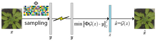
Figure 1.
The process of image acquisition based on deep CS. The image sensor compressed samples the original image and transmits the measurements to the base station. The image is reconstructed using the pre-trained generative network as prior information.
3.2. Generative Adversarial Networks with Variational Encoder
The framework of EnGe-CSNet proposed here is presented in Figure 2. is assumed as the set of all possible low dimension latent vectors. is set as the distribution of images, and is set as the distribution of latent vectors. As mentioned in [11], Generator, termed as called Decoder in VAE, is trained to learn a model that maximizes ,
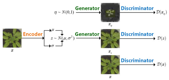
Figure 2.
The framework of EnGe-CSNet. The Encoder is used to find the low dimension latent vector of image . The Generator is used to reconstruct images. The Discriminator is used to distinguish real and erroneous images.
is considered the standard Gaussian prior distribution in DCGAN. In deep CS, more stress is placed on the vectors that more likely generate natural images. The Encoder is trained to learn a posterior probability distribution .
The problem that VAE tends to produce blurred images is solved by Discriminator (). It comprises three convolutional layers and two fully connected layers. Discriminator attempts to distinguish the real from the erroneous images. When Discriminator is being trained, the target score of real image is 1, and that of the image generated with vector sampled from standard Gaussian distribution is 0. As inspired by [10], cross-entropy acts as the loss function of Discriminator:
Generator () covers a fully connected layer and four deconvolutional layers. It is updated twice in each iteration. In the DCGAN process, image is generated using vector sampled from standard Gaussian distribution to fool Discriminator. When Generator is being trained, the target score of is 1. Thus, Equation (12) is derived as the loss function of the Generator in the DCGAN process:
In the VAE process, generates image with vector sampled from . It aims to make the Euclidean distance between and to be minimum. Thus, Equation (13) is derived as the loss function of the Generator trained in VAE process:
Encoder () comprises three convolutional layers and a fully connected layer. It finally outputs two vectors, i.e., a mean vector and a variance vector . is randomly sampled from the normal distribution . As derived in [24], latent loss of VAE is
where denotes the ith element of vector ; expresses the ith element of vector . Encoder aims to find the latent vector that makes approach and fool the Discriminator. Thus, Equation (15) is derived as the loss function of the Encoder:
Regularizer is introduced since Gaussian representation is selected for the latent prior and the approximate posterior .
4. Experiments and Discussion
4.1. Dataset and Training Details
The performance of the proposed model is tested with plant seedling and face images. The Aberystwyth leaf evaluation dataset contains four sets of 20 Arabidopsis Thaliana plants that have been grown in trays. Images of the respective tray are taken in a 15-min timelapse sequence. Interested readers can obtain this dataset from the following link: https://zenodo.org/record/168158#, accessed on 18 January 2021. CelebA is a large-scale face dataset with over 200,000 images involved. It can be obtained from this link: http://mmlab.ie.cuhk.edu.hk/projects/CelebA.html, accessed on 25 January 2021. For both datasets, we randomly sample 19,200 images for training, and 1000 for evaluation. In this study, each sample is cut from a large-scale image and scaled to an RGB image of size , giving inputs. The value of the respective input is scaled to .
The Encoder of EnGe-CSNet consists of three latent convolutional layers and one full connection output layer with a kernel size of , strides of 2. In the latent layers, acts as the activation function. The dimension of latent vector is set to . The Generator comprises one full connection layer and four transposed convolutional layers. Besides, all layers adopt the hyperbolic tangent function as activation. The discriminator consists of three convolutional layers and two full connection layers. All layers except for the output employ activation. Adam is employed to update all parameters of EnGe-CSNet with batch size 32 and learning rate 0.0001.
The optimizer of the reconstruction model refers to Adam with learning rate . This study searches up to times for the optimal low dimensional representation of each image. After the respective search step with iterations, the search will be terminated if , as the optimal solution is considered to be found.
The experiments’ hardware environment includes Intel(R) Xeon(R) W-2145 @3.70 GHz CPU, 64.0 GB DDR4 Memory, and NVIDIA Quadro RTX4000 GPU. The software environment is Windows 10 64-bit operating system, Python as the programming language, and Tensorflow2.0 as a library.
4.2. Comparisons with State-of-the-Art Approaches
4.2.1. Experimental Setup
For baselines, the proposed model is compared with Lasso [4], TVAL3 [25], NLRCS [26], DAMP [27], GAPTV [28] and CSGM [12]. The first five are optimization-based methods. The implementation codes of these algorithms are downloaded from authors’ websites. Lasso is applied to reconstruct images in WT domain because we found it perform better than in DCT domain. To reconstruct RGB images, we use CBM3D as the denoiser of DAMP. The RGB versions of TVAL3, NLRCS and GAPTV do not exist currently, so we reconstruct the three color channels independently. Other parameters for these methods, including the number of iterations, are set to the default values suggested by authors without any changes. CSGM is a reconstructed method based on generative models. The architecture of the generator in the CSGM is identical to EnGe-CSNet. According to [12], we optimize CSGM using Adam with a learning rate of 0.1 and do two random restarts with 500 update steps per restart and pick the reconstruction with the best measurement error.
The performance of the mentioned methods are tested at different compression rates (, that is, the ratio of the dimension of images and measurements ). The regularization parameters in Equation (8) are set to and in the experiments since these parameters are suggested to lead to the best performance according to experience. The parameters’ influence is discussed in Section 4.3. For all methods, the measurement matrix is a random Gaussian matrix with each entry sampled i.i.d from .
The Peak Signal to Noise Ratio (PSNR) and Structural Similarity (SSIM) are adopted for quantitative comparison. The PSNR is calculated by Equation (16).
where denotes the Mean Squared Error:
The SSIM is calculated by Equation (18).
where expresses the mean of , is the mean of , is the variance of , is the variance of , is covariance between and , and are constants that avoid dividing by zero.
4.2.2. Results and Discussion
Some visual examples reconstructed by various methods at the compression rate are illustrated in Figure 3 and Figure 4. Figure 3 gives four plant seedling images and Figure 4 shows four face images. Lasso’s reconstructed results are illegible. The results of TVAL3 are composed of many small color blocks, which makes the image unnatural. The reconstructed images of NLRCS and DAMP are excessively smooth and lose considerable useful information. As indicated from the face reconstruction results of GAPTV, there are numerous jagged edges in the image. CSGM is capable of reconstructing the outline of plants with high probability, whereas many details are lost. By comparison, The images reconstructed by the proposed model are much explicit than others with the compression rate . The edges of objects in images are easy to distinguish, which is more valuable information in applications. In terms of visual effect, the present study’s approach achieves better results.
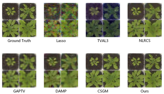
Figure 3.
Four examples of plant seedling images reconstructed by various methods. The compression rate is set to .
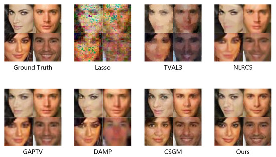
Figure 4.
Four examples of face images reconstructed by various methods. The compression rate is set to .
Table 1 lists the quantitative evaluations of different approaches. The average PSNR and SSIM at different compression rates on two test datasets are shown. The optimal results are marked in bold font. According to the quantitative results, the proposed model is significantly superior to six compared CS methods on plant seedling images. With a low compression rate of , the proposed model achieves the result similar to those achieved by NLRCS and DAMP. The PSNR&SSIM of three methods are 30.31&0.8110, 30.19&0.8044, 30.22&0.8098. The performance of the model here complies with the existing methods when there are sufficient measurements. However, the advantages gradually appear with the increase of compression rate. At the compression rate of 20, the PSNR&SSIM of NLRCS and DAMP decrease to 27.30&0.7014, 26.68&0.6780. But our method’s performance is almost maintained, the PSNR&SSIM are 30.01&0.8020. The performance of the proposed method on the face dataset is slightly worse than that on the plant seedling images, whereas it remains better than comparison methods at the high compression rate. DAMP achieves the best results with the PSNR&SSIM of 29.05&0.8506 at a compression rate of 10. Nevertheless its performance declines rapidly with the increase of compression rate. At , DAMP completely collapses, and the proposed model has PSNR&SSIM of 25.01&0.7492, which is significantly better than other methods. To be specific, when , the performance of the proposed model is highly consistent with CSGM’s on the face dataset because neither of them has sufficient information to reconstruct the high quality images. Yet both outperform other algorithms, which indicates that the compressed sensing method based on generative networks performs better at the high compression rate.

Table 1.
Average PSNR and SSIM comparisons of different image CS approaches. Bold indicates the best result.
The intuitive comparison presented in Figure 5 combines PSNR and SSIM. At the compression rate of 20, the SSIM of the proposed model reaches over 0.8 on both datasets, which is noticeably better than others. Moreover, Figure 3 and Figure 4 show that the proposed model retains more significant details. In brief, it is a more suitable method for specific applications of compressed sensing image reconstruction. With sufficient datasets, the proposed method is capable of obtaining high-quality images with meager sampling rates.
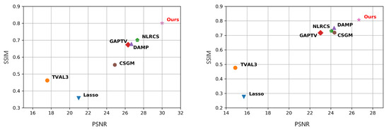
Figure 5.
Comparison of PSNR and SSIM at the compression rate of 20. The results of various methods on plant seedling images (left) and the CalebA dataset (right) are shown.
Table 2 shows the average runtimes of comparison methods on plant seedling images. The runtime is not the focus of our work because our method work on GPU while the first six baselines are implemented in MATLAB or scikit-learn and only utilize CPU. Our method runs faster than CSGM when the compression rate is low (e.g., and ) because it reconstructs high quality images with fewer restarts. It is hard to seek the optimal solution when the compression rate is high (e.g., ), so the proposed method costs more time than CSGM.
Table 2.
The average runtime (seconds) for each method with the variety of compression rates. Bold indicates the best result.
4.3. The Influence of Hyper-Parameters
Figure 6 shows the curves of the MSE of the reconstructed images using different hyper-parameters in Equation (9) with the number of iterations. In this subsection, the effect of and on the performance of our algorithm is mainly evaluated. The reconstructed model is considered over-fitting if the MSE decreases rapidly in the early stage of iteration but is finally maintained at a large value. It is considered under-fitting if the MSE decreases slowly and can not reach the minimum error. In Figure 6 (left), is set to 0.1 and is set to 0, 0.1, 0.5 respectively. It is shown that gives the best performance. The proposed method is over-fitting when and it is under-fitting when . In Figure 6 (right), is set to 0.1 and is set to 0, 0.1, 0.5, respectively. It is suggested that the three combinations exhibit the identical convergence rate at the early stage of iteration, but finally reaches the minimum test error. The proposed method is over-fitting when and it is under-fitting when . Hence, the recommended parameter combination here is , .
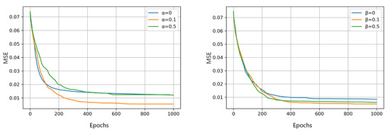
Figure 6.
The variety of average MSE test error with the increasing of epochs using 1000 plant seedling images. The influences of (left) and (right) in Equation (9) are presented.
4.4. Anti-Noise Performance
The images captured by sensors are commonly accompanied by noise. Several possible causes are presented as follows:
- The scene is insufficiently bright, or the brightness is non-uniform when the image sensor is operating.
- The temperature of image sensors is excessively high due to their long working time.
- Noise affecting the sensor’s circuit components may have an impact on the output image captured.
Accordingly, the image acquisition system should have strong anti-noise ability. The anti-noise performance is tested with Gaussian noise and salt-and-pepper noise. The image collected by the sensor is assumed below:
The algorithm aims to reconstructed image from measurements . The anti-noise performance is assessed by comparing the similarity between and . Figure 7 presents some reconstructed samples of various methods. Gaussian noise is added to seedling and face images.
where denotes the ratio of noise, is the Gaussian random noise, . As revealed from the visual comparison, the reconstructed image’s quality of the proposed approach is significantly higher than others. To be specific, the images reconstructed by TVAL3 and NLRCS are extremely blurry, which is even worse than noisy images. GAPTV is capable of recovering the target’s outline in general, whereas many color blocks cause the whole image lack details. DAMP achieves good results on several images, such as the female face, while other images are illegible. CSGM’s face reconstructed samples are unnatural. Though the outline is consistent with the ground truth, the details (e.g., eyes and mouth) are different. Besides, CSGM completely collapses while reconstructing the first plant seedling image. As opposed to the mentioned, the proposed model is more accurate in reconstructing image details and the edge of the target is clearer.
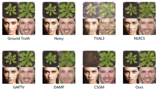
Figure 7.
Some reconstruction samples of plant seedling and face images adding Gaussian noise with and . The ground truth, noisy images, and images reconstructed by various methods are illustrated.
Table 3 shows the quantitative comparison of various methods with and . The best results are marked in bold font. The proposed method’s PSNR and SSIM are higher than others on both plant seedling and face datasets. As revealed from the evaluation, GAPTV also achieves good results, whereas the samples in Figure 7 reveal that its visual effect is poor.
Table 3.
Average PSNR and SSIM comparisons using images with Gaussian noise. Bold indicates the best result.
In another experiment, salt-and-pepper (i.e., pixel loss) noise is added to images.
where denotes the ratio of pixels lost, and abides by the uniform distribution between 0 and 1. Figure 8 presents some reconstructed samples and Table 4 gives the quantitative evaluation with and . The results on images with salt-and-pepper noise provide the identical conclusion as that of images with Gaussian noise. In brief, the proposed model’s anti-noise performance is significantly better than that of other methods, and the model has strong robustness.
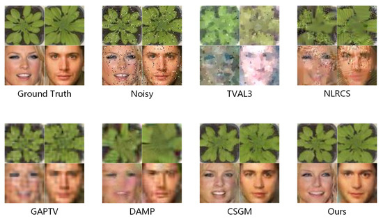
Figure 8.
Some reconstruction samples of plant seedling and face images adding salt-and-pepper noise with and . The ground truth, noisy images, and images reconstructed by various methods are illustrated.
Table 4.
Average PSNR and SSIM comparisons using images with salt-and-pepper noise. Bold indicates the best result.
5. Conclusions
In this study, a deep CS model is proposed and introduced to specific CS applications (e.g., plant seedling or face images acquisition). The proposed model is capable of reconstructing images more effectively than existing models, significantly reducing the amount of data to be transmitted. As verified by experiments on both datasets, the performance of the method proposed here outperforms existing algorithms. The major advantage of the proposed algorithm is that it can effectively reconstruct the images at high compression rates (above 20). Thanks to convolutional neural networks, it is a data-driven method. Thus, another important advantage is that, with the increase of the training set, the generative model’s performance will be enhanced and the details of images can be restored more effectively. It also exhibits strong anti-noise ability. For the mentioned reason, it is a more practical method.
Moreover, the reconstruction of images exhibiting complex backgrounds is an open question. Given the different characteristics of the target and background, multiple generative networks are considered helpful. The recovering of details refers to another question. In subsequent studies, we will introduce some post-processing methods to improve reconstruction performance in depth.
Author Contributions
Conceptualization, B.Z. and J.Z.; methodology, B.Z.; software, B.Z.; validation, J.Z.; formal analysis, B.Z.; investigation, X.R.; resources, X.R.; data curation, J.Z.; writing—original draft preparation, B.Z.; writing—review and editing, G.S.; supervision, G.S.; project administration, G.S. All authors have read and agreed to the published version of the manuscript.
Funding
This work was supported by the National Natural Science Foundation of China (No.61771262), Tianjin Science and Technology Major Project and Engineering (No.18ZXRHNC00140).
Data Availability Statement
All data generated or analyzed during this study are included in this article.
Acknowledgments
The authors would like to thank Tianjin Key Laboratory of Optoelectronic Sensor and Sensor Network Technology for providing working conditions.
Conflicts of Interest
The authors declare no conflict of interest.
References
- Donoho, D.L. Compressed sensing. IEEE Trans. Inf. Theory 2006, 52, 1289–1306. [Google Scholar] [CrossRef]
- Fracastoro, G.; Fosson, S.M.; Magli, E. Steerable discrete cosine transform. IEEE Trans. Image Process. 2016, 26, 303–314. [Google Scholar] [CrossRef]
- Rein, S.; Reisslein, M. Scalable line-based wavelet image coding in wireless sensor networks. J. Vis. Commun. Image Represent. 2016, 40, 418–431. [Google Scholar] [CrossRef]
- Candes, E.J.; Tao, T. Decoding by linear programming. IEEE Trans. Inf. Theory 2005, 51, 4203–4215. [Google Scholar] [CrossRef]
- Candes, E.J. The restricted isometry property and its implications for compressed sensing. C. R. Math. 2008, 346, 589–592. [Google Scholar] [CrossRef]
- Raskutti, G.; Wainwright, M.J.; Yu, B. Restricted eigenvalue properties for correlated Gaussian designs. J. Mach. Learn. Res. 2010, 11, 2241–2259. [Google Scholar]
- Tropp, J.A.; Gilbert, A.C. Signal recovery from random measurements via orthogonal matching pursuit. IEEE Trans. Inf. Theory 2007, 53, 4655–4666. [Google Scholar] [CrossRef]
- Bickel, P.J.; Ritov, Y.; Tsybakov, A.B. Simultaneous analysis of Lasso and Dantzig selector. Ann. Stat. 2009, 37, 1705–1732. [Google Scholar] [CrossRef]
- Ji, S.; Xue, Y.; Carin, L. Bayesian compressive sensing. IEEE Trans. Signal Process. 2008, 56, 2346–2356. [Google Scholar] [CrossRef]
- Radford, A.; Metz, L.; Chintala, S. Unsupervised representation learning with deep convolutional generative adversarial networks. arXiv 2015, arXiv:1511.06434. [Google Scholar]
- Kingma, D.P.; Welling, M. Auto-encoding variational bayes. arXiv 2013, arXiv:1312.6114. [Google Scholar]
- Bora, A.; Jalal, A.; Price, E.; Dimakis, A.G. Compressed sensing using generative models. In Proceedings of the International Conference on Machine Learning, Sydney, Australia, 6–11 August 2017; pp. 537–546. [Google Scholar]
- Larsen, A.B.L.; Sønderby, S.K.; Larochelle, H.; Winther, O. Autoencoding beyond pixels using a learned similarity metric. In Proceedings of the International Conference on Machine Learning, New York, NY, USA, 19–24 June 2016; pp. 1558–1566. [Google Scholar]
- Bell, J.; Dee, H. Aberystwyth leaf evaluation dataset. 2016, 168158, 2. Available online: https://doi.org/10.5281/zenodo (accessed on 18 January 2021).
- Liu, Z.; Luo, P.; Wang, X.; Tang, X. Deep learning face attributes in the wild. In Proceedings of the IEEE International Conference on Computer Vision, Santiago, Chile, 7–13 December 2015; pp. 3730–3738. [Google Scholar]
- Chartrand, R.; Yin, W. Iteratively reweighted algorithms for compressive sensing. In Proceedings of the 2008 IEEE International Conference on Acoustics, Speech and Signal Processing, Las Vegas, NV, USA, 31 March–4 April 2008; pp. 3869–3872. [Google Scholar]
- Zhang, J.; Xiong, T.; Tran, T.; Chin, S.; Etienne-Cummings, R. Compact all-CMOS spatiotemporal compressive sensing video camera with pixel-wise coded exposure. Opt. Express 2016, 24, 9013–9024. [Google Scholar] [CrossRef] [PubMed]
- Kwan, C.; Gribben, D.; Chou, B.; Budavari, B.; Larkin, J.; Rangamani, A.; Tran, T.; Zhang, J.; Etienne-Cummings, R. Real-Time and Deep Learning Based Vehicle Detection and Classification Using Pixel-Wise Code Exposure Measurements. Electronics 2020, 9, 1014. [Google Scholar] [CrossRef]
- Wu, Y.; Rosca, M.; Lillicrap, T. Deep compressed sensing. arXiv 2019, arXiv:1905.06723. [Google Scholar]
- Shi, W.; Jiang, F.; Liu, S.; Zhao, D. Image Compressed Sensing Using Convolutional Neural Network. IEEE Trans. Image Process. 2019, 29, 375–388. [Google Scholar] [CrossRef] [PubMed]
- Yang, Y.; Sun, J.; Li, H.; Xu, Z. ADMM-CSNet: A deep learning approach for image compressive sensing. IEEE Trans. Pattern Anal. Mach. Intell. 2018, 42, 521–538. [Google Scholar] [CrossRef]
- Seitzer, M.; Yang, G.; Schlemper, J.; Oktay, O.; Würfl, T.; Christlein, V.; Wong, T.; Mohiaddin, R.; Firmin, D.; Keegan, J.; et al. Adversarial and perceptual refinement for compressed sensing MRI reconstruction. In Proceedings of the International Conference on Medical Image Computing and Computer-Assisted Intervention, Granada, Spain, 16–20 September 2018; pp. 232–240. [Google Scholar]
- Kingma, D.P.; Ba, J. Adam: A method for stochastic optimization. arXiv 2014, arXiv:1412.6980. [Google Scholar]
- Odaibo, S. Tutorial: Deriving the Standard Variational Autoencoder (VAE) Loss Function. arXiv 2019, arXiv:1907.08956. [Google Scholar]
- Li, C.; Yin, W.; Jiang, H.; Zhang, Y. An efficient augmented Lagrangian method with applications to total variation minimization. Comput. Optim. Appl. 2013, 56, 507–530. [Google Scholar] [CrossRef]
- Dong, W.; Shi, G.; Li, X.; Ma, Y.; Huang, F. Compressive sensing via nonlocal low-rank regularization. IEEE Trans. Image Process. 2014, 23, 3618–3632. [Google Scholar] [CrossRef]
- Metzler, C.A.; Maleki, A.; Baraniuk, R.G. From denoising to compressed sensing. IEEE Trans. Inf. Theory 2016, 62, 5117–5144. [Google Scholar] [CrossRef]
- Yuan, X. Generalized alternating projection based total variation minimization for compressive sensing. In Proceedings of the 2016 IEEE International Conference on Image Processing (ICIP), Phoenix, AZ, USA, 25–28 September 2016; pp. 2539–2543. [Google Scholar]


Publisher’s Note: MDPI stays neutral with regard to jurisdictional claims in published maps and institutional affiliations. |
© 2021 by the authors. Licensee MDPI, Basel, Switzerland. This article is an open access article distributed under the terms and conditions of the Creative Commons Attribution (CC BY) license (https://creativecommons.org/licenses/by/4.0/).