3.1. Numerical Simulations
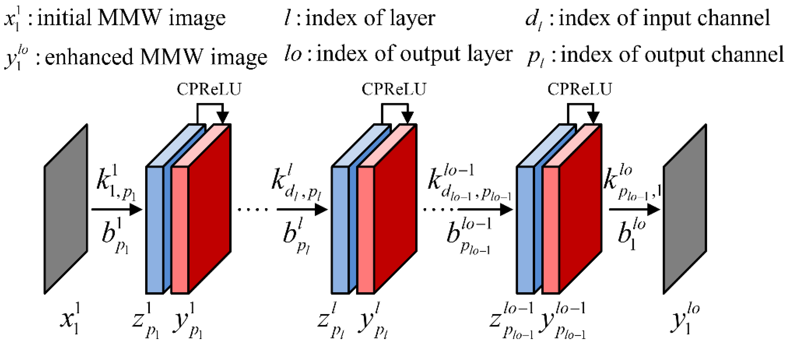
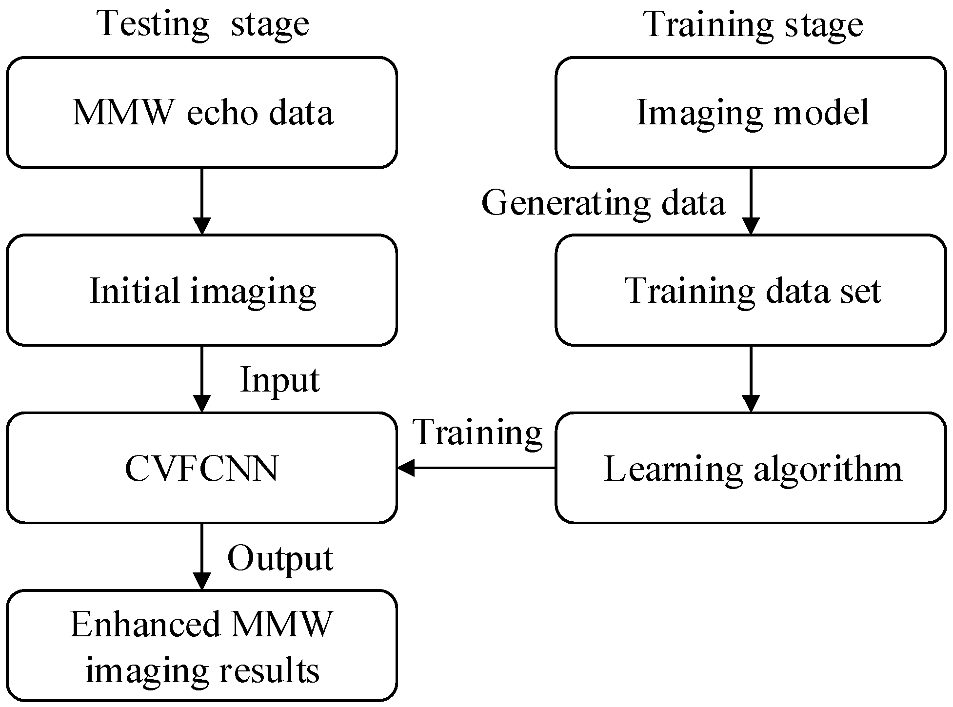
The structures of several enhanced imaging approaches, based on CNN and CS, are shown in
Figure 4. The phase shift migration (PSM) algorithm is used for the initial imaging, also known as the range stacking technique [
37,
38,
39,
40]. The variables CConv and Conv represent the complex and real convolutions, respectively. In the CS method, we employ the PSM operator-based CS algorithm given in [
37] with the constraints of
l1-norm and TV-norm. Next, we will provide comparisons of these methods through simulations and experiments.
The parameters for generating the simulated dataset are shown in
Table 1. The data generation method is similar to that used in [
30], but we generate the initial images using the PSM algorithm. In addition, both the initial images and the ground-truth images contain phases. For different sampling rates, 2048 groups of simulated data are generated respectively, including pairs of initial images and ground-truth images. Among them, 1920 groups of data are used as the training set, and the remaining 128 groups are treated as the testing dataset. The above neural networks are trained using the same initialization parameters. RVFCNN is initialized by the real and imaginary parts of CVFCNN. The method of momentum stochastic gradient descent with weight decay is used to update the network parameters. The momentum factor is set to be 0.5 for all parameters. For the parameters of convolution kernels and biases, the weight decay coefficient is 0.001 and the learning rate is 6 × 10
−6. The parameters of CPReLU and PReLU are initialized to be 0.25 without weight decay, and the learning rate is 6 × 10
−4. We trained for 8 epochs with a batch size of 16. The networks were programmed based on MATLAB, implemented on a computer platform with an Intel Xeon E5-2687W v4 CPU.
The networks are randomly initialized 5 times during training,
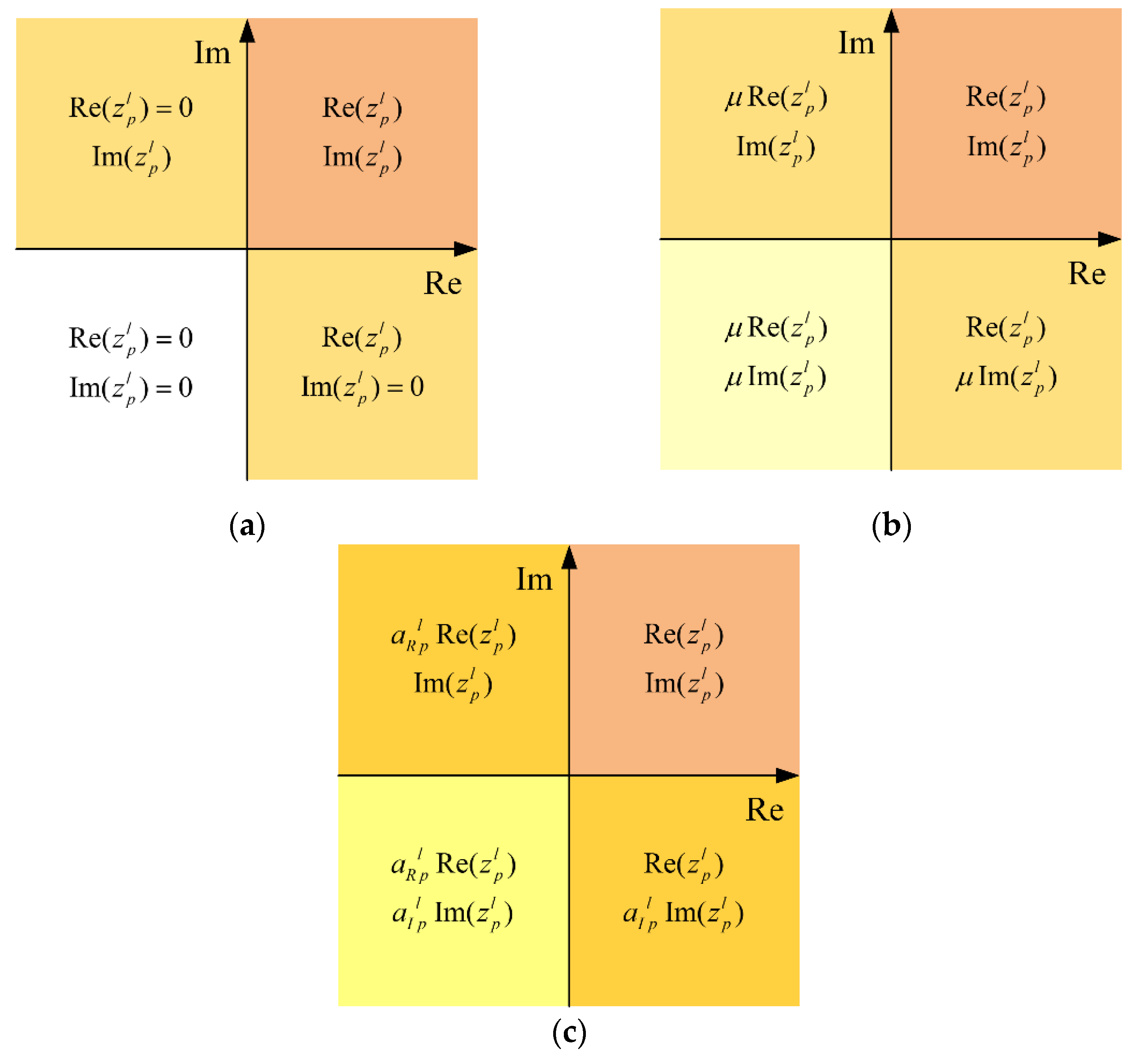
Table 2 shows the average for the sum of the squared errors between the imaging results and the ground-truth images on the testing dataset. CPReLU
1 represents the CPReLU demonstrated in [
31] with constant parameters, and the parameters are set as the initial value, i.e., 0.25. CPReLU
2 refers to the proposed adaptive CPReLU, with independent real and imaginary parameters. Note that the neural network methods outperform both the traditional PSM method and the CS method with respect to different data ratios. The proposed CVFCNN (CPReLU
2) possesses the minimum number of errors among the neural network methods. We also note that the parameters of RVFCNN are twice those of CVFCNN [
28]. Specifically, CVFCNN (CPReLU
1) and CVFCNN (CPReLU
2) contain 38,032 real numbers, CVFCNN (CReLU) contains 37,936 real numbers, and RVFCNN (PReLU) contains 75,968 real numbers in this example. However, RVFCNN does not perform better. The CVFCNN (CPReLU
1) has relatively poor performance, which means it is unreliable to directly set a constant value as the parameter of CPReLU
1. Similarly, the performance of CReLU is also inferior to that of CPReLU
2, due to being without adaptive parameter adjustments.
The training time for different network architectures is shown in
Table 3. We note that CVFCNN (CReLU) has the fastest training speed since the CReLU contains operations including zero. RVFCNN (PReLU) contains more channels, so the training speed is slow. The proposed CVFCNN (CPReLU
2) is slightly slower than CVFCNN (CReLU) and CVFCNN (CPReLU
1) because the parameters of the CPReLU
2 activation function need to be updated adaptively during the training stage. However, in general, people pay more attention to the processing time of the testing stage, as shown in
Table 4.
Table 4 indicates the average processing time for a single image, where GPU time means the time spent when we input the image obtained by the PSM algorithm into the neural network and evaluate the processing time on the GPU. The NVIDIA TITAN Xp card is utilized to record the GPU time. Note that the neural network methods run much faster than the CS method, due to being without iterations. In addition, in terms of CS methods, we need to readjust the parameters for different types of targets, while CNN-based methods can obtain results very rapidly after training the parameters of the network. The processing time of the proposed CVFCNN (CPReLU
2) on the CPU is slightly longer than that of CVFCNN (CReLU) but with a lower SSE, as shown in
Table 2. Usually, in order to obtain a better-quality image, the cost of a little processing time could be ignored. In addition, when processed by the GPU, the processing time difference between CVFCNN (CPReLU
2) and CVFCNN (CReLU) in this simulation experiment is very small, being less than 0.01 s.
3.2. Results of the Measured Data
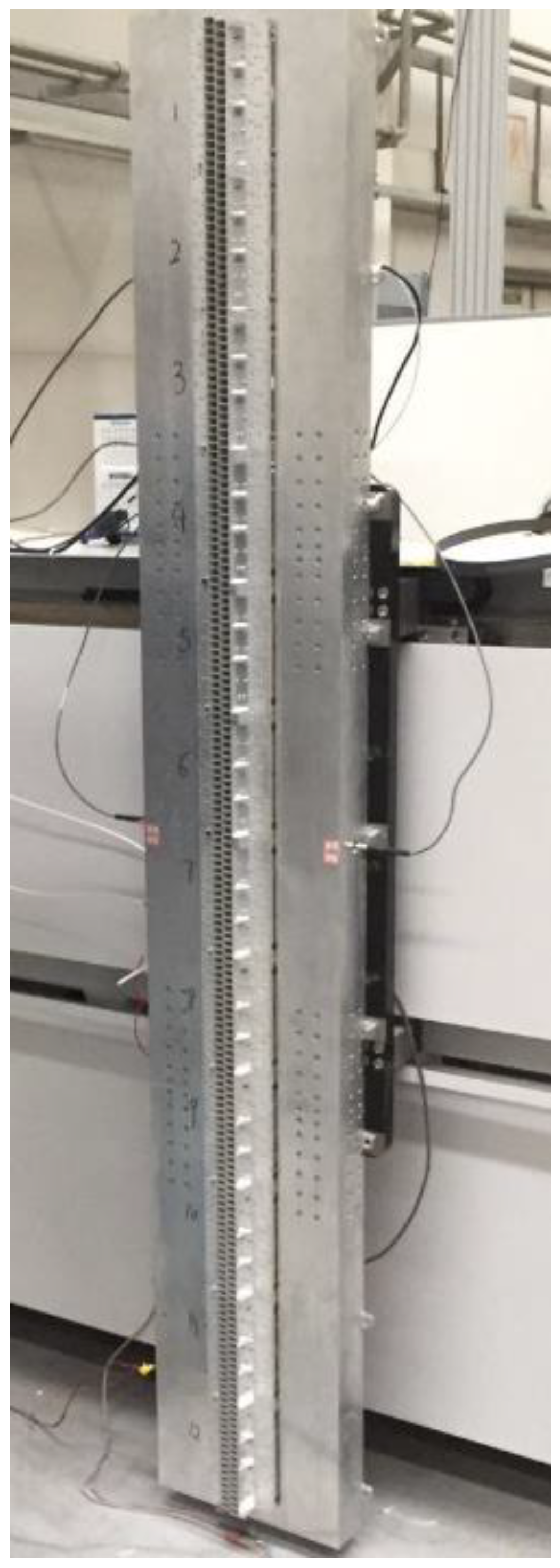
Here, we present experiments on the real measured data by a Ka band system operating at 32~37 GHz, as shown in
Figure 5. The wide-band linear array forms a 2-D aperture through mechanical scanning. The parameters for the measured data are provided in
Table 5. The measured targets are located at different distances from the antenna array, as shown in
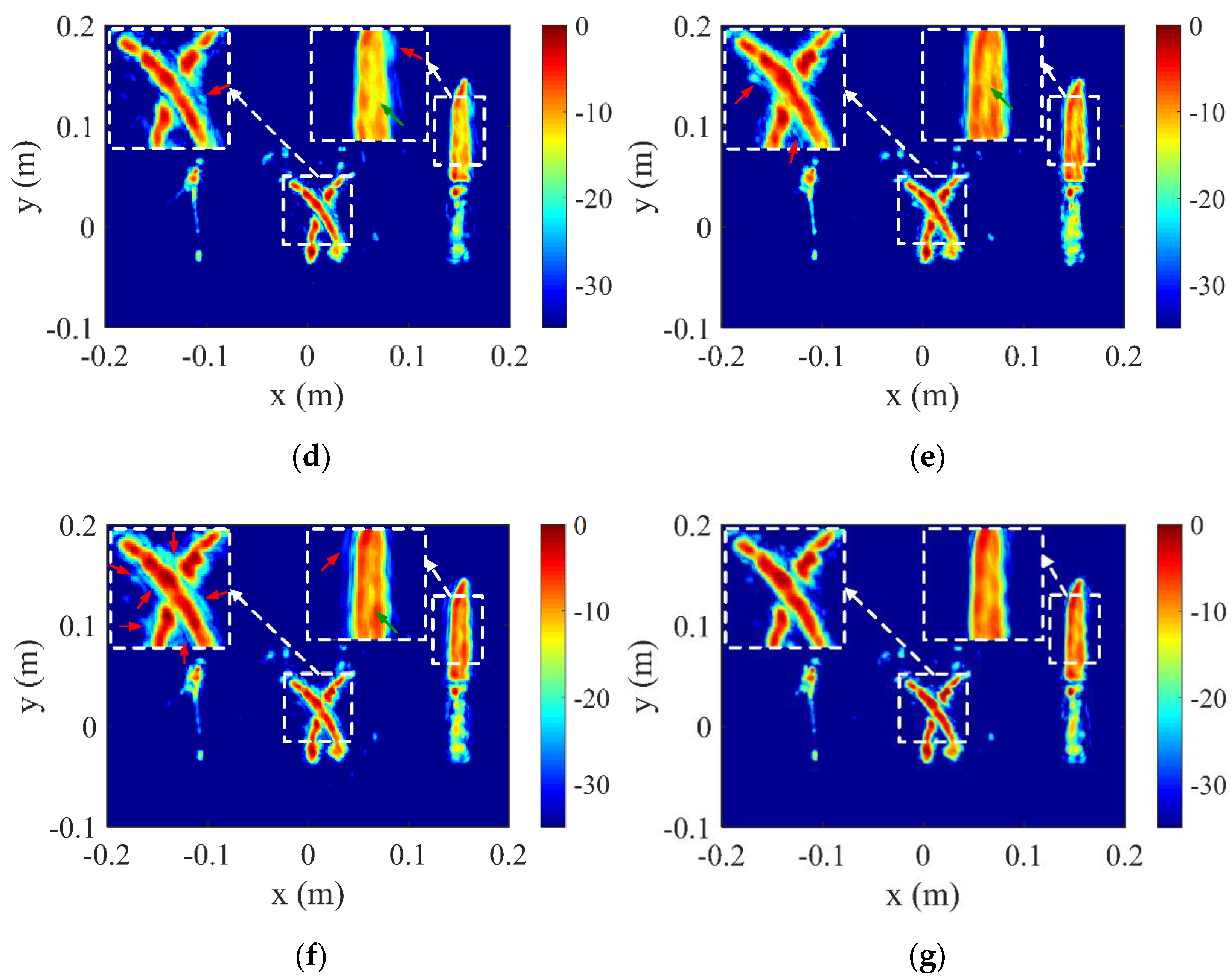
Figure 6a. The 2-D images are obtained through the maximum value projection of the 3-D results.
Figure 6b demonstrates the imaging result of the PSM, using only 50% of the full data.
Figure 6c illustrates the result of the CS method after repeated artificial parameter optimization. It can be seen that in order to suppress the aliasing artifacts and sidelobes of the image, the amplitudes of the targets are weakened; the parameters of the CS algorithm need to be adjusted according to the states of the scenes and the objects.
Figure 6d–g shows the results of the CNN methods. Note that the CNN methods can achieve better results than the traditional PSM algorithm and perform competitively with the CS method or are even better, especially for the amplitude maintenance of the image. More importantly, CNN methods have strong robustness in terms of different objects and scenes in the testing stage. In regard to the CNN methods, as indicated by the green arrows, the amplitudes of the knife blade of CPReLU
1 (
Figure 6f) and CPReLU
2 (
Figure 6g) are more uniform than those of PReLU (
Figure 6d) and CReLU (
Figure 6e). Note from the detailed subfigures that the result of the proposed CPReLU
2 in
Figure 6g exhibits lower sidelobes than the results in
Figure 6d–f, respectively, wherein the sidelobes are indicated by red arrows. The experimental results show that the proposed CPReLU
2 performs best of the tested methods.
Table 6 shows the processing time of each algorithm for the measured data, which is similar to the results on the simulated testing dataset in
Table 4. In the processing of measured data, the CNN-based methods are much faster than the CS method. In addition, the CNN method exhibits stronger robustness in the testing stage, and the CS method needs to readjust the algorithm parameters for different objects and scenes. The processing time of the proposed CVFCNN (CPReLU
2) is slightly longer than that of CVFCNN (CReLU) but yielded better imaging results, as shown in
Figure 6. Usually, in order to obtain a better-quality image, the cost of a little processing time could be ignored.


 ,
, 


