
A Frequency and Voltage Coordinated Control Strategy of Island Microgrid including Electric Vehicles

 ,
, 
 ,
,
Abstract
:1. Introduction
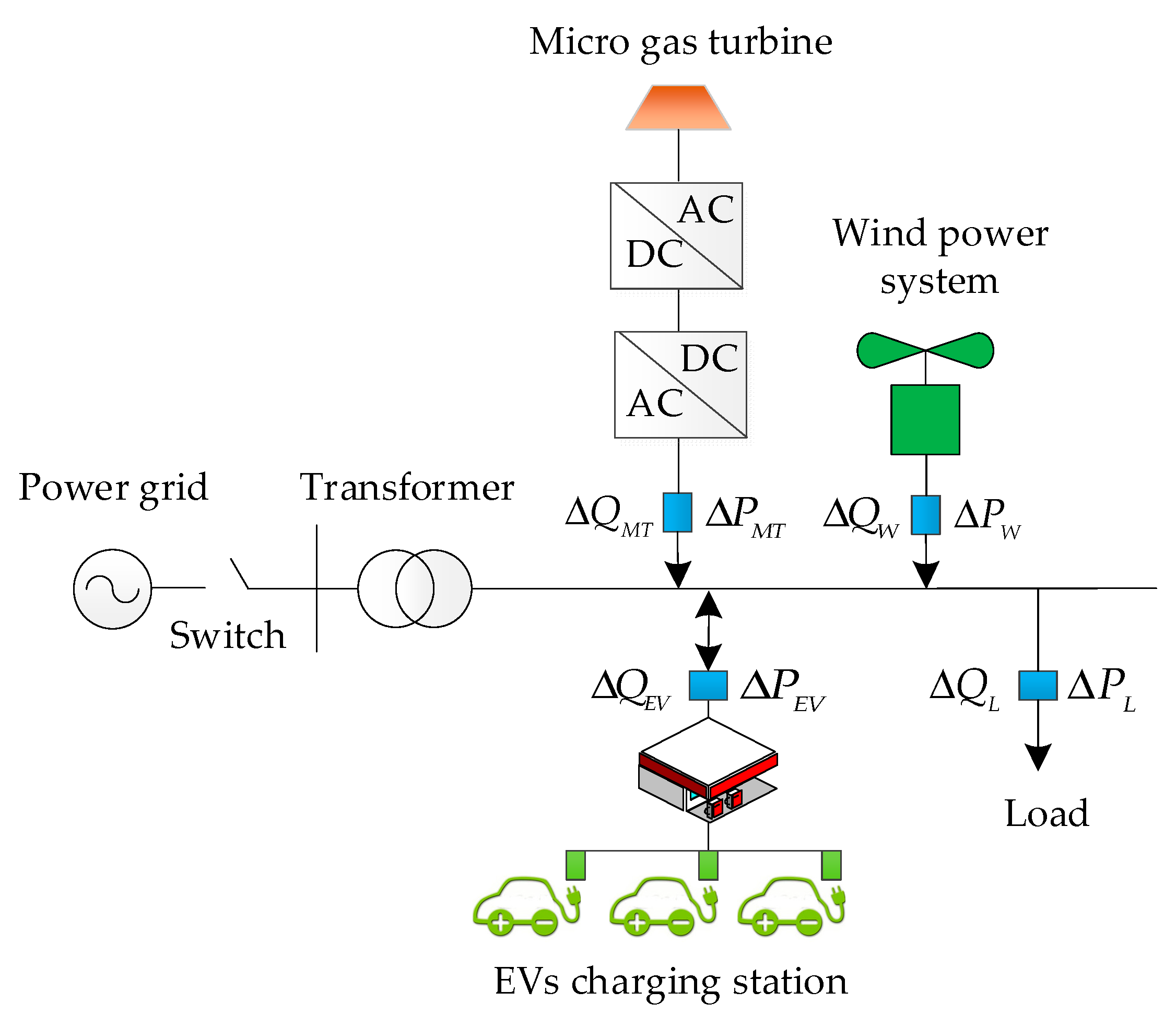
2. Microgrid Control Model with EVs
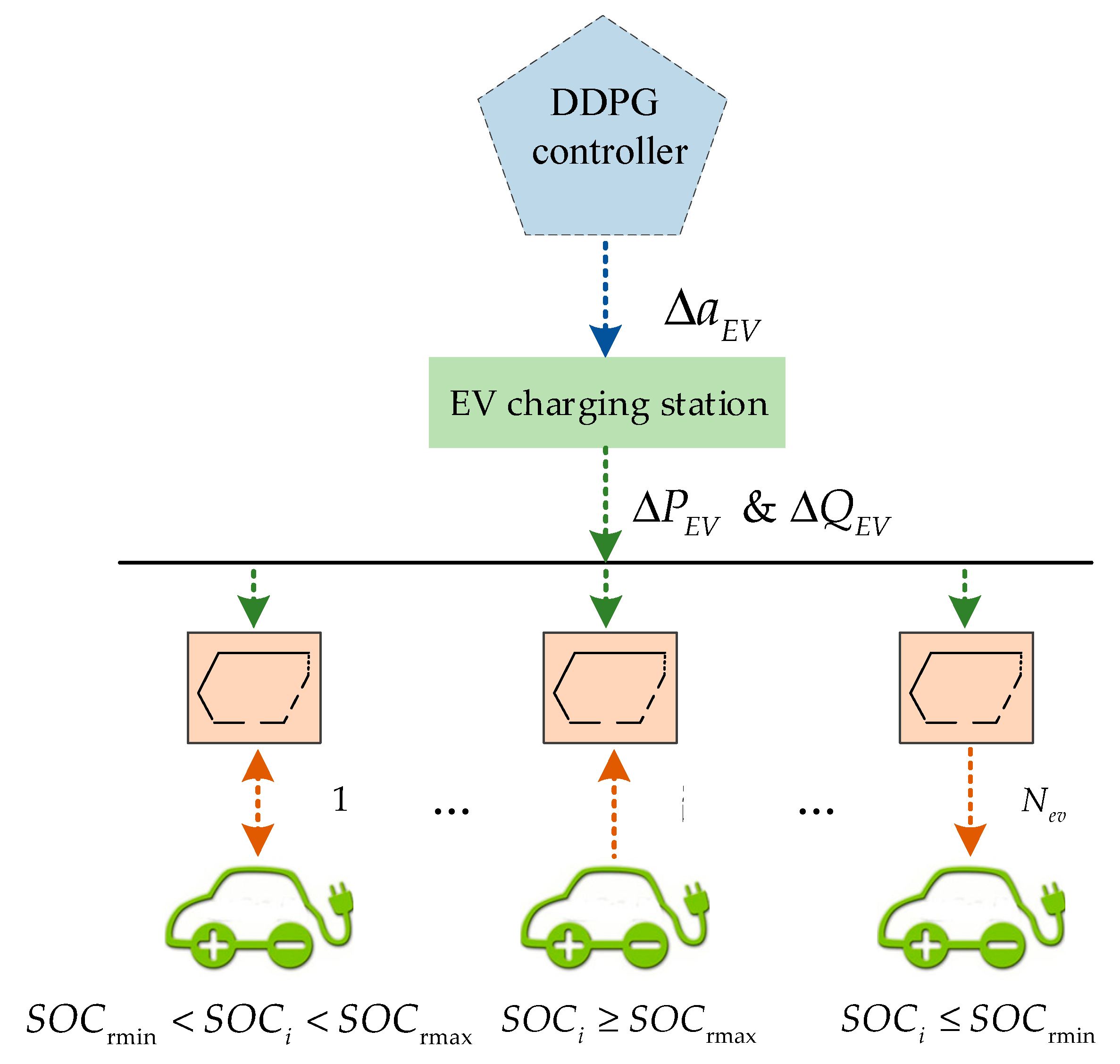
2.1. Electric Vehicle Control Model
2.2. VF Control Model of Microgrids with EVs
3. The Design of Microgrid VF Controller Based on DDPG
3.1. Theoretical Analysis of DDPG
3.2. Design of DDPG VF Controller Structure
3.3. Definition of Space and Reward Function
3.4. The Selection of Hyperparameter
3.5. Summary of Control Strategy
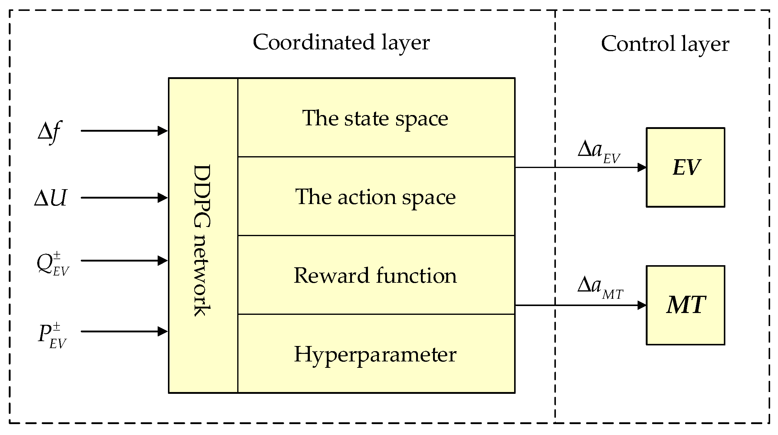
- Firstly, definite the state set of the control system as ∆F(t), ∆U(t), and . In addition, the action space can be defined as ∆AP,MT (t), ∆AP,EV (t), ∆AQ,MT (t), ∆Aφ,EV (t).
- Secondly, the parameters are adjusted according to the actual calculation example, and the values of the reward function coefficients and hyperparameters are obtained.
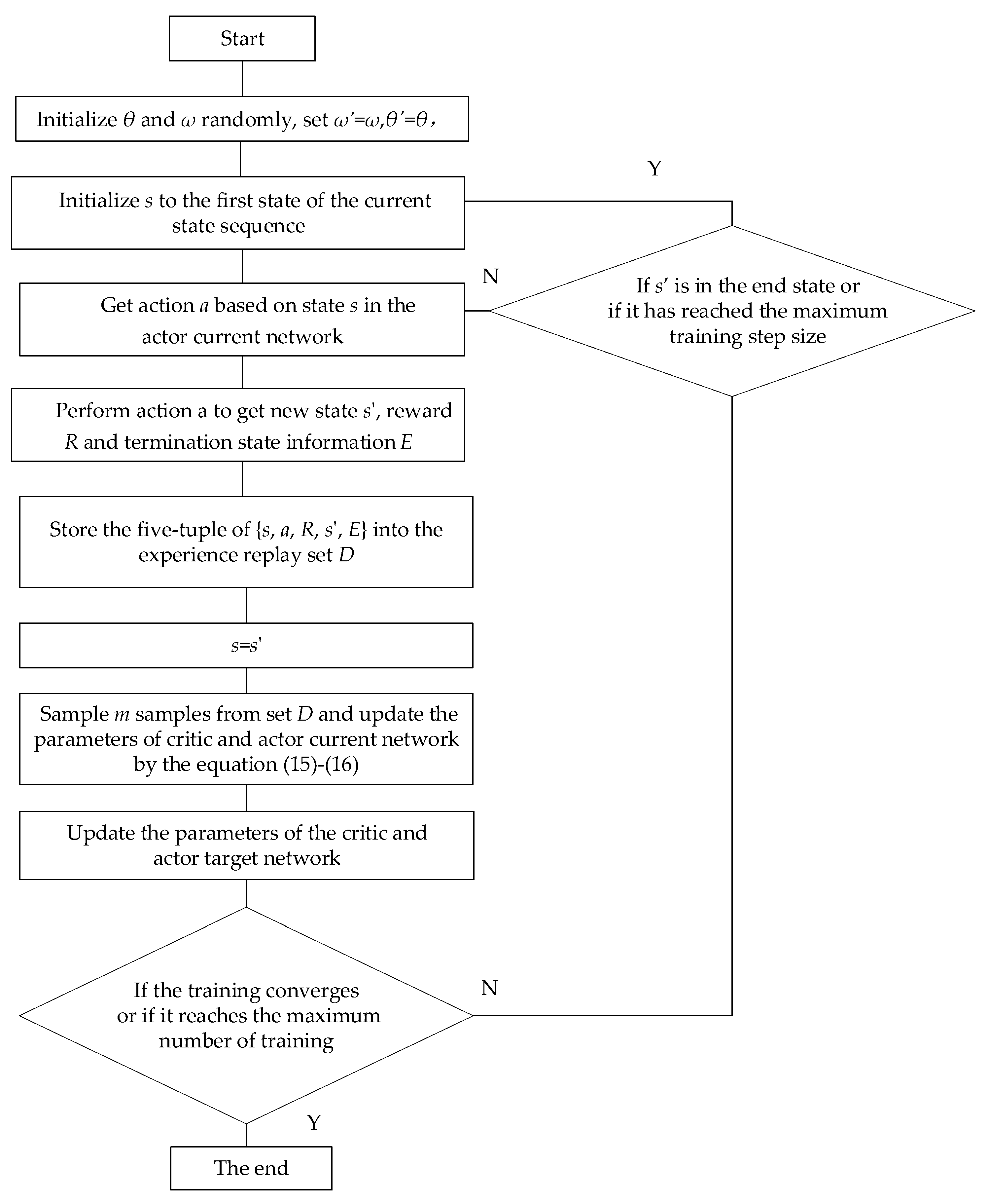
- Thirdly, perform agent training according to the process in Figure 5, and obtain the optimal value function Q network Qφ(s,a).
- Finally, in different cases, input disturbances to the islanded microgrid system, and the agent can generate corresponding actions based on the disturbances to adjust the output of each unit, so as to ensure the frequency and voltage balance of the islanded microgrid system.
4. Simulation Results
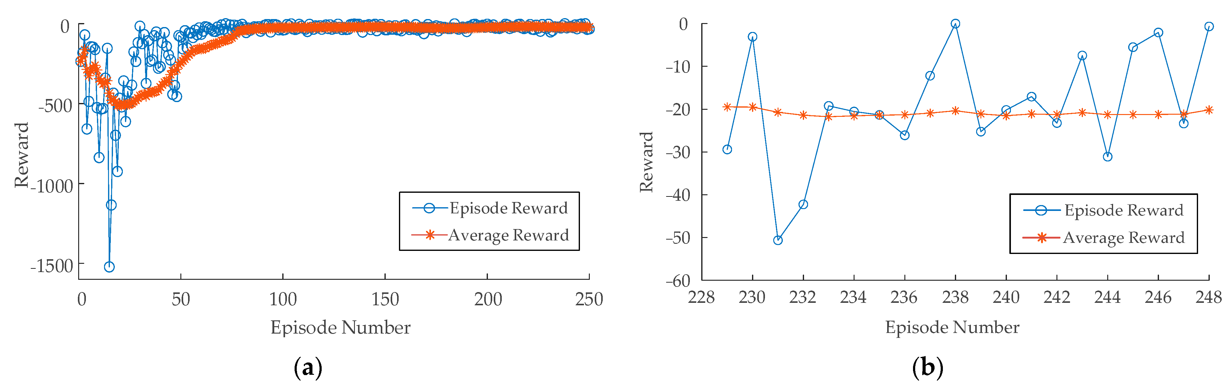
4.1. Pre-Learning Stage
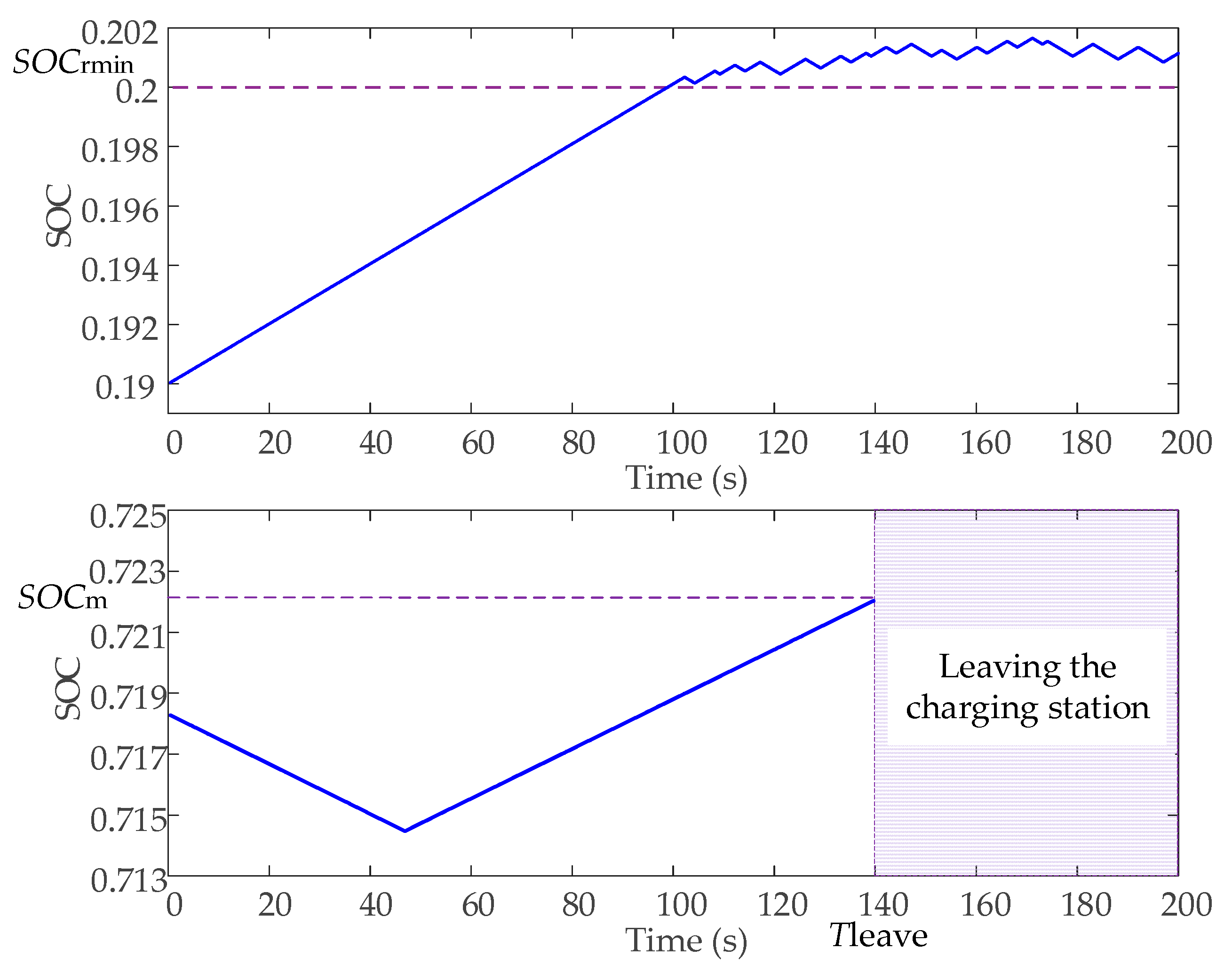
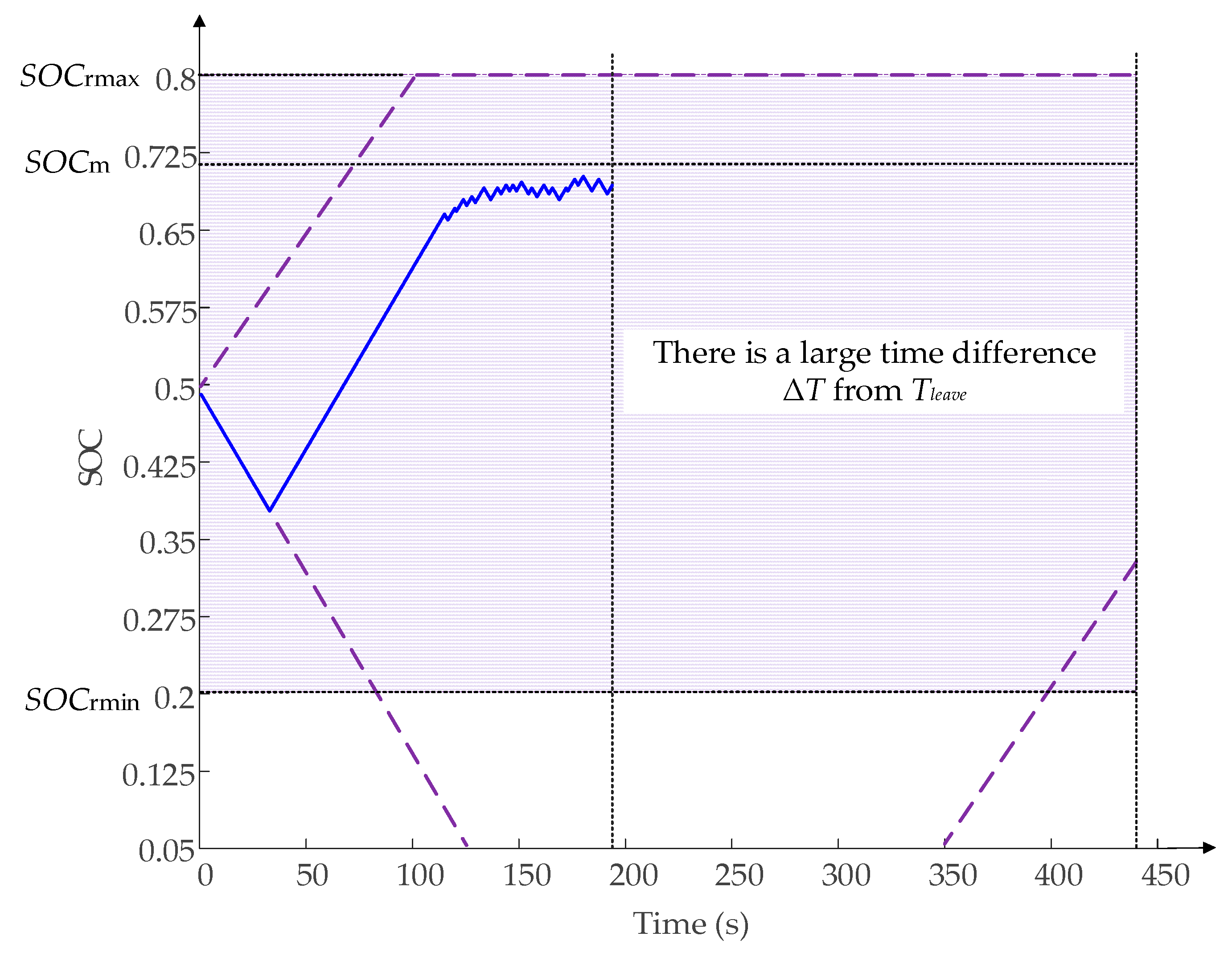
4.2. The Implementation of Constraint Conditions in the EV Model
4.3. Case Study
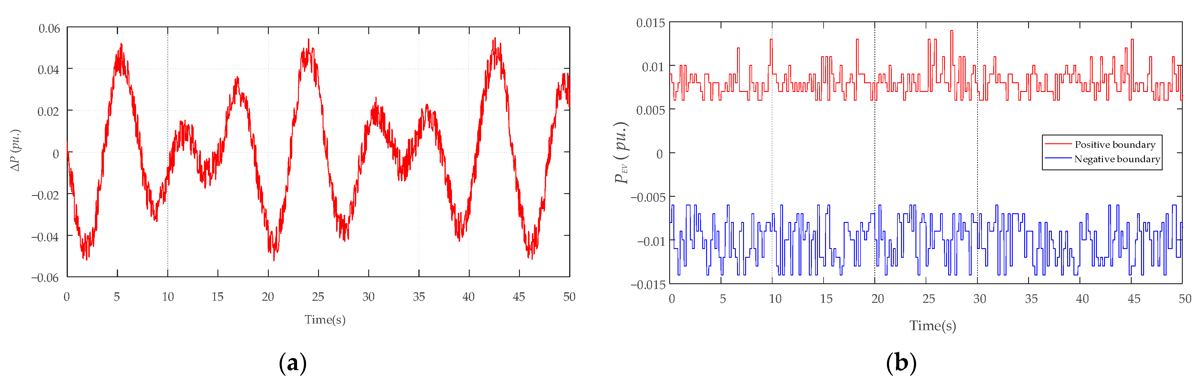
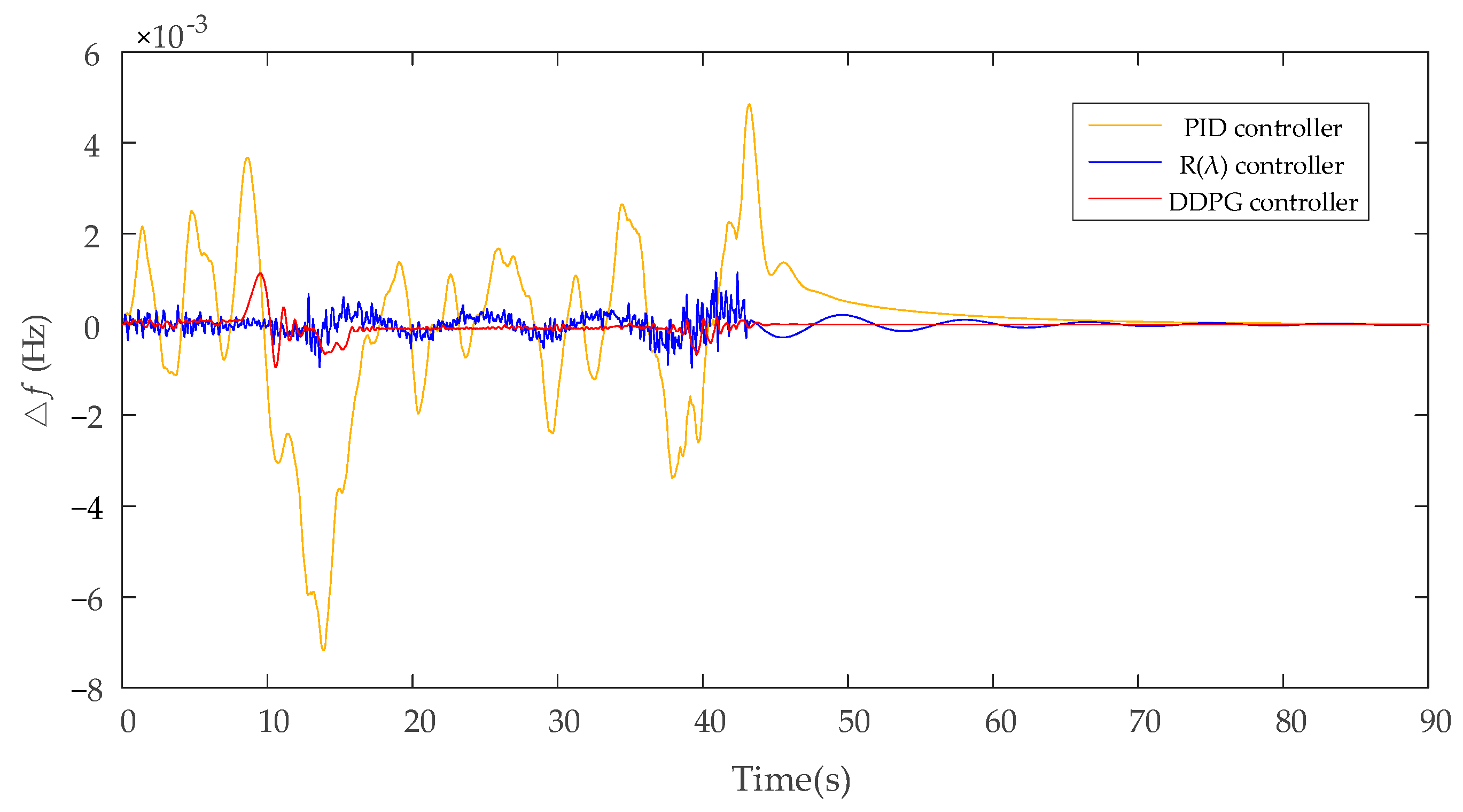
4.3.1. Case 1: The Response of Wind Power Disturbance
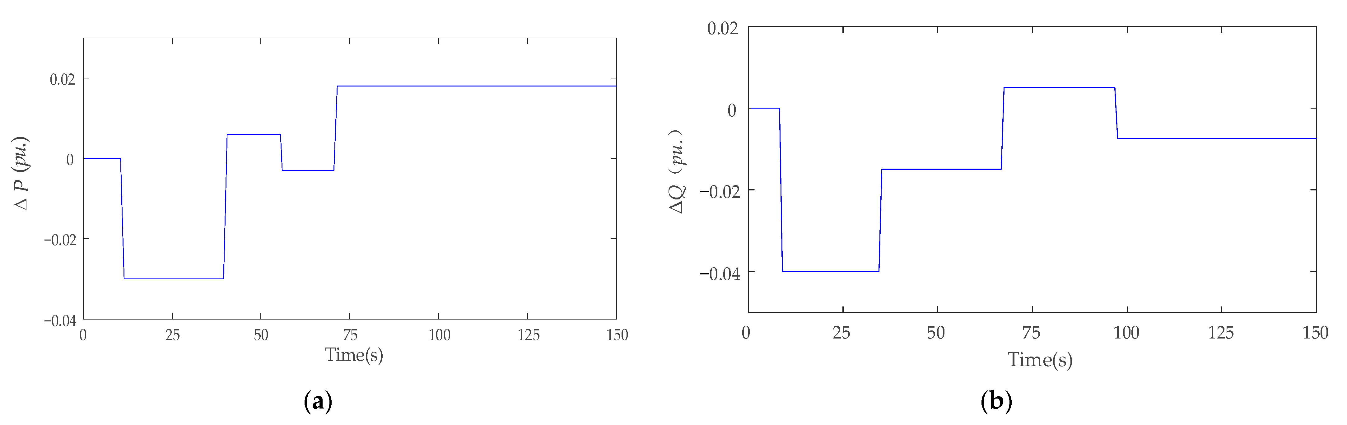
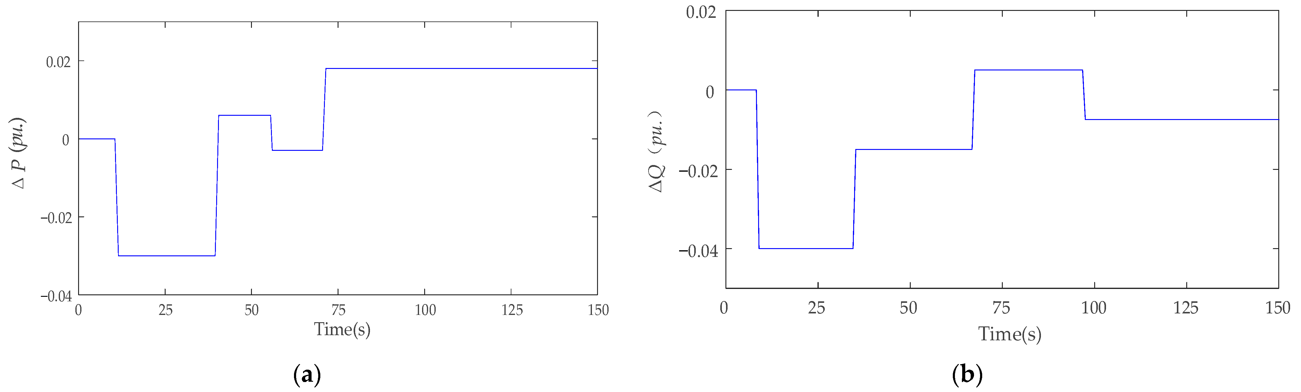
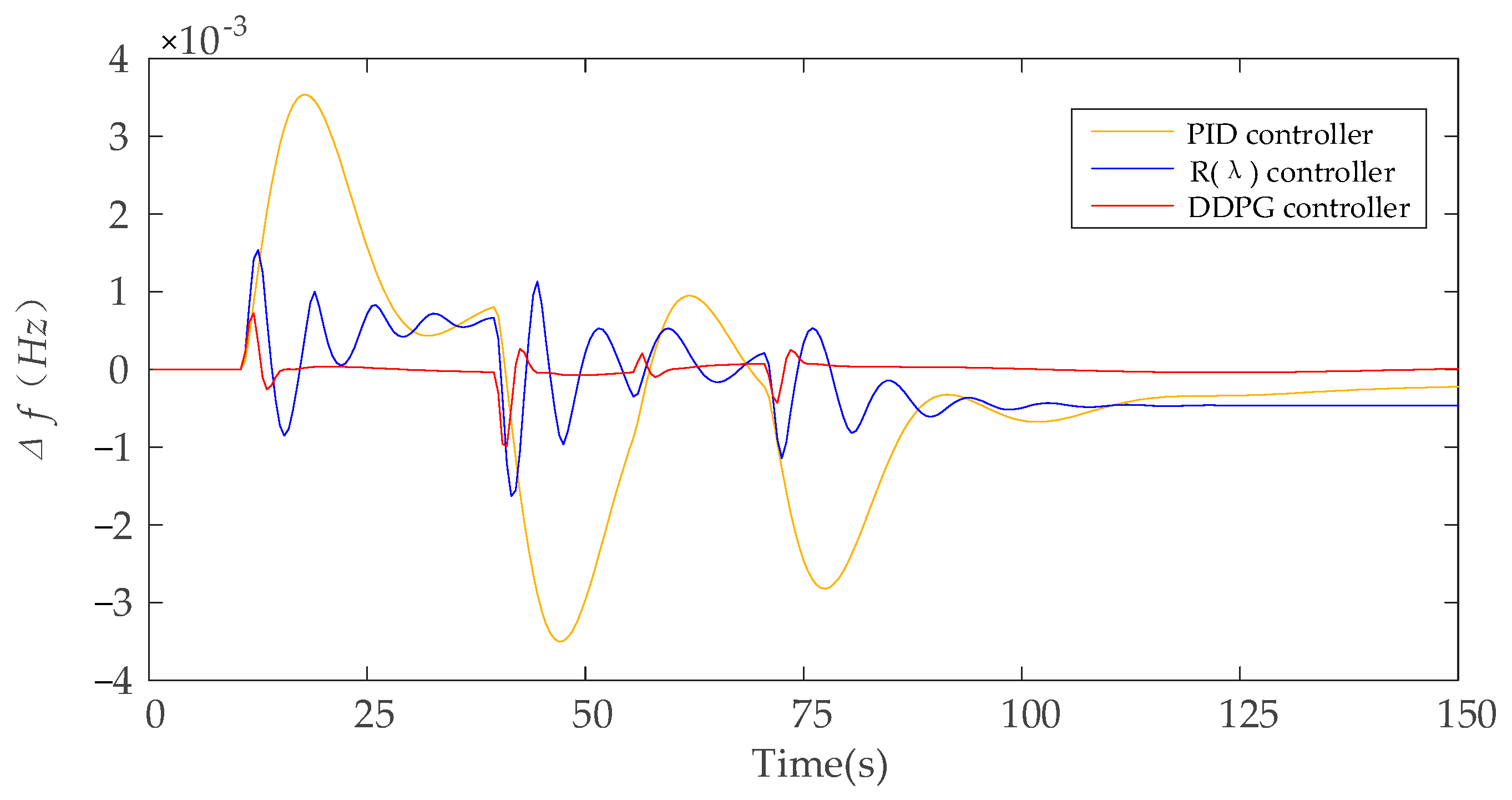
4.3.2. Case 2: The Response to Load Power Disturbance
5. Conclusions
- Compared with PID controller, the DDPG controller with the ability of online learning and experience playback can more effectively deal with the highly random disturbance. Under the wind disturbance, the frequency fluctuation of the islanded microgrid under the DDPG controller can be limited in 2 × 10⁻⁴ Hz, and the excellent rate can reach 98%, which is significantly better than the traditional controller.
- Compared with the R(λ) controller, the DDPG controller in this paper can coordinate the frequency recovery and voltage adjustment of the island microgrid, so as to meet the VF control requirements at the same time, which is more suitable for the stable control of the microgrid. When the load changes, the DDPG controller can ensure that the frequency deviation of the microgrid is maintained within ±1 × 10⁻³ Hz, and the voltage deviation is also close to 0.
- The EV charging station has the characteristics of small inertia and fast regulation speed in the microgrid control, which can play an important role in VF regulation;
- The realization effect of the constraint conditions in the EV model is great. The single EV can judge whether it participates in the adjustment of the microgrid system according to the SOC situation.
Author Contributions
Funding
Conflicts of Interest
References
- Lam, Q.L.; Bratcu, A.I.; Riu, D.; Boudinet, C.; Labonne, A.; Thomas, M. Primary frequency H_∞ control in stand-alone mi-crogrids with storage units: A robustness analysis confirmed by real-time experiments. Int. J. Electr. Power Energy Syst. 2020, 115, 105507.1–105507.13. [Google Scholar] [CrossRef]
- Chae, S.; Kim, G.; Choi, Y.-J.; Kim, E.-H. Design of Isolated Microgrid System Considering Controllable EV Charging Demand. Sustainability 2020, 12, 9746. [Google Scholar] [CrossRef]
- Ziras, C.; Prostejovsky, A.M.; Bindner, H.W.; Marinelli, M. Decentralized and discretized control for storage systems offering primary frequency control. Electr. Power Syst. Res. 2019, 177, 106000.1–106000.10. [Google Scholar] [CrossRef] [Green Version]
- Roudbari, E.S.; Beheshti, M.T.H.; Rakhtala, M. Voltage and frequency regulation in islandeded microgrid with PEM fuel cell based on a fuzzy logic voltage control and adaptive droop control. IET Power Electron. 2019, 13, 78–85. [Google Scholar] [CrossRef]
- Joung, K.W.; Kim, T.; Park, J.W. Decoupled frequency and voltage control for stand-alone microgrid with high renewable penetration. In Proceedings of the IEEE/IAS Industrial & Commercial Power Systems Technical Conference IEEE, Niagara Falls, ON, Canada, 7–10 May 2018. [Google Scholar]
- Dhua, R.; Goswami, S.K.; Chatterjee, D. An Optimized Frequency and Voltage Control Scheme for Distributed Generation Units of an Islandeded Microgrid. In Proceedings of the 2021 Innovations in Energy Management and Renewable Resources (IEMRE), Kolkata, India, 5–7 February 2021. [Google Scholar]
- Keypour, R.; Adineh, B.; Khooban, M.H.; Blaabjerg, F. A New Population-Based Optimization Method for Online Minimiza-tion of Voltage Harmonics in Islandeded Microgrids. IEEE Trans. Circuits Syst. II: Express Briefs 2019, 67, 1084–1088. [Google Scholar] [CrossRef]
- Wang, C.; Mei, S.; Dong, Q.; Chen, R.; Zhu, B. Coordinated Load Shedding Control Scheme for Recovering Frequency in Is-landeded Microgrids. IEEE Access 2020, 8, 215388–215398. [Google Scholar] [CrossRef]
- Iqbal, S.; Xin, A.; Jan, M.U.; Salman, S.; Abdelbaky, M.A. V2G Strategy for Primary Frequency Control of an Industrial Mi-crogrid Considering the Charging Station Operator. Electronics 2020, 9, 549. [Google Scholar] [CrossRef] [Green Version]
- Fan, H.; Lin, J.; Zhang, C.K.; Mao, C. Frequency regulation of multi-area power systems with plug-in electric vehicles con-sidering communication delays. IET Gener. Transm. Distrib. 2016, 10, 3481–3491. [Google Scholar] [CrossRef] [Green Version]
- Yang, J.; Zeng, Z.; Tang, Y.; He, H.; Wu, Y. Load Frequency Control in Isolated Micro-Grids with Electrical Vehicles Based on Multivariable Generalized Predictive Theory. Energies 2015, 8, 2145–2164. [Google Scholar] [CrossRef]
- Rao, Y.; Yang, J.; Xiao, J.; Xu, B.; Liu, W.; Li, Y. A frequency control strategy for multi-microgrids with V2G based on the im-proved robust model predictive control. Energy 2021, 222, 119963.1–119963.13. [Google Scholar] [CrossRef]
- Li, P.; Hu, W.; Xu, X.; Huang, Q.; Liu, Z.; Chen, Z. A frequency control strategy of electric vehicles in microgrid using virtual synchronous generator control. Energy 2019, 189, 116389. [Google Scholar] [CrossRef]
- Kisacikoglu, M.C.; Ozpineci, B.; Tolbert, L. EV/PHEV Bidirectional Charger Assessment for V2G Reactive Power Operation. IEEE Trans. Power Electron. 2013, 28, 5717–5727. [Google Scholar] [CrossRef]
- Cao, Y.; Tang, S.; Li, C.; Zhang, P.; Tan, Y.; Zhang, Z.; Li, J. An Optimized EV Charging Model Considering TOU Price and SOC Curve. IEEE Trans. Smart Grid 2011, 3, 388–393. [Google Scholar] [CrossRef]
- U.S. U.S. Department of Transportation. Federal Highway Administration, 2017 National Household Travel Survey. Available online: http://nhts.ornl.gov (accessed on 20 November 2021).
- Gjelaj, M.; Hashemi, S.; Andersen, P.B.; Traeholt, C. Optimal infrastructure planning for EV fast-charging stations based on prediction of user behaviour. IET Electr. Syst. Transp. 2020, 10, 1–12. [Google Scholar] [CrossRef] [Green Version]
- Mojdehi, M.N.; Ghosh, P. An On-Demand Compensation Function for an EV as a Reactive Power Service Provider. IEEE Trans. Veh. Technol. 2015, 65, 4572–4583. [Google Scholar] [CrossRef]
- Vachirasricirikul, S.; Ngamroo, I. Robust LFC in a Smart Grid with Wind Power Penetration by Coordinated V2G Control and Frequency Controller. IEEE Trans. Smart Grid 2014, 5, 371–380. [Google Scholar] [CrossRef]
- Zhu, X.; Xia, M.; Chiang, H.-D. Coordinated sectional droop charging control for EV aggregator enhancing frequency stability of microgrid with high penetration of renewable energy sources. Appl. Energy 2018, 210, 936–943. [Google Scholar] [CrossRef]
- Zhang, J.; Zhang, C.; Chien, W.C. Overview of Deep Reinforcement Learning Improvements and Applications. J. Internet Technol. 2021, 22, 239–255. [Google Scholar]
- Giannopoulos, A.; Spantideas, S.; Kapsalis, N.; Karkazis, P.; Trakadas, P. Deep Reinforcement Learning for Energy-Efficient Multi-Channel Transmissions in 5G Cognitive HetNets: Centralized, Decentralized and Transfer Learning Based Solutions. IEEE Access 2021, 9, 129358–129374. [Google Scholar] [CrossRef]
- Yang, Q.; Zhu, Y.; Zhang, J.; Qiao, S.; Liu, J. UAV Air Combat Autonomous Maneuver Decision Based on DDPG Algorithm. In Proceedings of the 2019 IEEE 15th International Conference on Control and Automation (ICCA) IEEE, Edinburgh, Scotland, 16–19 July 2019. [Google Scholar]
- Gulde, R.; Tuscher, M.; Csiszar, A.; Riedel, O.; Verl, A. Deep reinforcement learning using cyclical learning rates. In Proceedings of the 2020 Third International Conference on Artificial Intelligence for Industries (AI4I), Irvine, CA, USA, 21–23 September 2020. [Google Scholar]
- Yu, T.; Zhou, B.; Chan, K.W.; Yuan, Y.; Yang, B.; Wu, Q.H. R(λ) imitation learning for automatic generation control of in-terconnected power grids. Automatica 2012, 48, 2130–2136. [Google Scholar] [CrossRef]


| Unit | Parameter | Meaning | Value |
|---|---|---|---|
| MT | time constant of governor | 10 s | |
| time constant of generator | 0.1 s | ||
| speed regulation factor | 0.005 Hz/p.u. | ||
| lower limit of active power variation | −0.025 p.u. | ||
| upper limit of active power variation | 0.025 p.u. | ||
| lower limit of reactive power variation | −0.025 p.u. | ||
| upper limit of reactive power variation | 0.03 p.u. | ||
| EV1 | time constant of EV | 1 s | |
| lower limit of active power variation | −0.016 p.u. | ||
| upper limit of active power variation | 0.016 p.u. | ||
| lower limit of reactive power variation | −0.015 p.u. | ||
| upper limit of reactive power variation | 0.015 p.u. | ||
| nEV1 | Initial number of EVs in station1 | 40 | |
| EV2 | time constant of EV | 1.5 s | |
| lower limit of active power variation | −0.014 p.u. | ||
| upper limit of active power variation | 0.014 p.u. | ||
| lower limit of reactive power variation | −0.0135 p.u. | ||
| upper limit of reactive power variation | 0.0135 p.u. | ||
| nEV2 | Initial number of EVs in station2 | 35 |
| SN | Parameter Settings | Average Reward | Final Award |
|---|---|---|---|
| 1 | h = 3, u = 50 | −34.037 | −1.83622 |
| 2 | h = 3, u = 200 | −26.673 | −1.20923 |
| 3 | h = 5, u = 50 | −21.096 | −0.65307 |
| 4 | h = 5, u = 200 | −27.075 | −1.35723 |
| 5 | h = 10, u = 50 | −34.572 | −2.54778 |
| 6 | h = 10, u = 200 | −40.922 | −3.04643 |
| Controller | Describe | Parameter | Value |
|---|---|---|---|
| PID | Proportional gain | KP | 4 |
| Integral gain | Ki | 1.18 | |
| Differential gain | KD | 0.5 | |
| R(λ) | learning rate | α | 0.01 |
| discount factor | γ | 0.9 | |
| network depth | (h, u) | (3, 10) |
| Indicators | PID | R(λ) | DDPG |
|---|---|---|---|
| Average (Hz) | 0.9215 × 10⁻³ | 0.1159 × 10⁻³ | 0.0267 × 10⁻³ |
| Maximum (Hz) | 7.174 × 10⁻³ | 1.148 × 10⁻³ | 1.133 × 10⁻³ |
| Proficiency (%) | 30.56% | 92.07% | 98.35% |
| Trecover (s) | 34.25 | 23.95 | 0.75 |
| Indicators | PID | R(λ) | DDPG |
|---|---|---|---|
| Average (Hz) | 0.995 × 10⁻³ | 0.437 × 10⁻³ | 0.0521 × 10⁻³ |
| Maximum (Hz) | 3.54 × 10⁻³ | 1.63 × 10⁻³ | 1.09 × 10⁻³ |
| Proficiency (%) | 9.6% | 16.7% | 98% |
| Trecover (s) | / | / | 0.13 |
| Indicators | PID | R(λ) | DDPG |
|---|---|---|---|
| Average (p.u) | 0.0093 | 0.0021 | 0.00047 |
| Maximum (p.u) | 0.0569 | 0.0112 | 0.0023 |
| Proficiency (%) | 30.3% | 83.07% | 100% |
| Trecover (s) | / | / | 9.2 |
Publisher’s Note: MDPI stays neutral with regard to jurisdictional claims in published maps and institutional affiliations. |
© 2021 by the authors. Licensee MDPI, Basel, Switzerland. This article is an open access article distributed under the terms and conditions of the Creative Commons Attribution (CC BY) license (https://creativecommons.org/licenses/by/4.0/).
Share and Cite
Fan, P.; Ke, S.; Kamel, S.; Yang, J.; Li, Y.; Xiao, J.; Xu, B.; Rashed, G.I. A Frequency and Voltage Coordinated Control Strategy of Island Microgrid including Electric Vehicles. Electronics 2022, 11, 17. https://doi.org/10.3390/electronics11010017
Fan P, Ke S, Kamel S, Yang J, Li Y, Xiao J, Xu B, Rashed GI. A Frequency and Voltage Coordinated Control Strategy of Island Microgrid including Electric Vehicles. Electronics. 2022; 11(1):17. https://doi.org/10.3390/electronics11010017
Chicago/Turabian StyleFan, Peixiao, Song Ke, Salah Kamel, Jun Yang, Yonghui Li, Jinxing Xiao, Bingyan Xu, and Ghamgeen Izat Rashed. 2022. "A Frequency and Voltage Coordinated Control Strategy of Island Microgrid including Electric Vehicles" Electronics 11, no. 1: 17. https://doi.org/10.3390/electronics11010017
APA StyleFan, P., Ke, S., Kamel, S., Yang, J., Li, Y., Xiao, J., Xu, B., & Rashed, G. I. (2022). A Frequency and Voltage Coordinated Control Strategy of Island Microgrid including Electric Vehicles. Electronics, 11(1), 17. https://doi.org/10.3390/electronics11010017