Time Delay Estimation Control of Permanent Magnet Spherical Actuator Based on Gradient Compensation

Abstract

A multi-degree-of-freedom Permanent Magnet Spherical Actuator (PMSpA) has a special mechanical structure and electromagnetic fields, and is easily affected by nonlinear disturbances such as modeling errors and friction. Therefore, the quality of a PMSpA control system may be deteriorated. In order to keep the PMSpA with good trajectory tracking performance, this paper designs a time delay estimation controller based on gradient compensation. Firstly, the dynamic model of the PMSpA with nonlinear terms is derived. The nonlinear terms in the complex dynamic model can be simplified and estimated by the time delay estimation method. Secondly, for the estimation errors caused by time delay control, a gradient compensator is introduced to further correct and compensate for it. Furthermore, the stability of the designed controller is proved by the Lyapunov equation. Finally, the correctness and effectiveness of the controller are validated by comparison with other controllers through simulation. In addition, experimental results have also shown that the control accuracy of the spherical motor can be effectively improved using the proposed controller.

1. Introduction

Usually, the multiple dimensional motion on a single axis must be achieved by multiple single-shaft motors and complex mechanical transmission mechanisms. However, this will increase the weight, volume, and design cost of the system, reduce stiffness and dynamic performance, and generate working singularity. By contrast, the novel spherical motor can realize three degree-of-freedom (DOF) of motion at one node. It has broad potential applications in essential fields such as robotics, industrial manufacturing, and precision assembly [1,2,3]. In [4], the shell-like induction motor was concretized as a traction motor in an electric wheel-chair. In [5], the concept of a spherical-motor-based motion platform for providing high performance nozzle-substrate negotiation in conformal printing of curved electronics was presented. The spherical motor has become a research focus worldwide.

In the process of research in recent decades, spherical motors with various structures and principles such as induction, permanent magnet (PM), and ultrasonic have been produced [6,7,8]. The spherical motors usually refer to the multi-DOF motors with spherical rotors. As for the permanent magnet spherical motor in [7], its rotor is composed of two spherical surfaces, on which the PM poles are distributed symmetrically. It is worth noting that the distribution of stator coils and the PM poles are extended into three dimensional space. The magnetic field interacts with the current input in the stator coils and creates torque vectors in the space to move the rotor in 3-DOF.

This paper mainly studies a Permanent Magnet Spherical Actuator (PMSpA) with a compact structure. The control goal of the spherical motor is to make the rotor output shaft reach a continuous trajectory from the initial position to any desired position. For fulfilling such a purpose, scholars have proposed many control algorithms. In [9,10], the Proportional Derivative (PD) control method was put forward. The PD controller is simple and easy to design, but it requires a large control torque to compensate for uncertainties and external disturbances and has a certain degree of conservatism. In [11], a Computational Torque Control (CTC) method was proposed to linearize and decouple the dynamic model. However, this method is a model-based method, and the control accuracy will be affected in the presence of uncertainty, friction, and external disturbances. In addition, scholars have proposed adaptive control [12,13], neural network identifier-based control [14], sliding mode control [15], decoupling control [16], and other intelligent control methods, but these controllers have a complicated structure and are cumbersome in the gain adjustment process, which are not convenient for practical applications.

A time delay estimation control method with a simple structure and good robustness was proposed for the tracking problem of robot systems with the unknown dynamic model [17]. The main idea of this control method is to estimate unknown and difficult nonlinear terms in complex dynamic equations by using the values of delayed input torque and acceleration. The time delay estimation control has been widely used in mechanical systems and control schemes because of its simple control system and relatively simple control gain selection.

However, when the nonlinear disturbances such as friction and external disturbance exist in the system, the performance of time delay estimation control will be degraded. This will result in large estimation errors and affect the control effect [18]. In [19], a time delay estimation control method with ideal speed feedback for systems was designed to compensate for the estimation errors. The speed feedback is used to eliminate the nonlinear term that cannot be offset by the time delay estimation control. However, it is difficult for the speed feedback to correct the estimation errors caused by various uncertain disturbances, and the robustness of the system is poor. In [20,21,22], a sliding mode controller is added to the time delay estimation control to reduce estimation errors. However, the implementation of the sliding mode control algorithm needs to know the upper bound of disturbance, and it is easy to cause the chattering of the position tracking response and output torque, which will affect the motor body. In [23], a method combining time delay estimation control with fuzzy logic was put forward, which uses fuzzy logic to eliminate nonlinear terms, but fuzzy control will make the system complicated and increase the amount of calculation. Although the above methods can effectively suppress the time delay estimation errors, more control gain will make the system complicated, and the control gain adjustment is time-consuming, which will increase the burden of actual controller design.

Considering the nonlinear uncertainty and strong coupling of PMSpA body structure and dynamic model [24], this paper has proposed the time delay estimation control method based on gradient compensation (TDGEC), which deals with unknown and nonlinear terms in complex dynamic equations through time delay estimation, and at the same time uses gradient compensation to reduce the estimation errors caused by time delay estimation control. The simple structure of the proposed controller can improve the tracking effect of the complex nonlinear PMSpA motion control system and avoid the complicated gain adjustment process. Finally, the PD control method, CTC method, and traditional Time Delay Estimation Control (TDC) are used for simulation and experimental comparison with the proposed controller.

The remainder of this paper is organized as follows. In Section 2, the structure and dynamic model of the PMSpA are introduced. In Section 3, a time delay estimation controller with gradient estimation is designed, and the stability of the control system is verified based on the Lyapunov method. The PD controller, CTC controller, and TDC controller are used to simulate and compare with the proposed control algorithm in Section 4. Section 5 introduces the experimental platform and carries on verification on the experimental platform. Finally, conclusions are made in Section 6.

2. Structure and Dynamic Model of PMSpA

2.1. Mechanical Structure of PMSpA

Figure 1 is the structure diagram of the PMSpA, which is composed of a spherical rotor, and two hemispherical shells [25]. Four layers of cylindrical PMs are evenly embedded on the rotor. There are 40 PMs in total, and the two poles are alternately distributed. There are two layers of stator coils on the stator shell symmetrically distributed along the equator, and each layer contains 12 equidistant air-core coils.

The principle diagram of PMSpA movement is shown in Figure 2. The interaction between the energized coils and the PMs of the rotor generates an electromagnetic torque. By energizing the stator coil according to a particular energization strategy, the PMSpA can realize three-DOF of spin, pitch, and yaw motion. The specifications of the PMSpA are shown in

Table 1. Specifications of the PMSpA.

Parameters	Unit	Value
Radius of the stator	mm	115
Radius of the rotor	mm	64
Height of coils	mm	25
Inner radius of coils	mm	4
Ampere-turns coils	A	1200
Radius of PMs	mm	10
Length of air gap	mm	1
Material of PM		NdFe35
Maximum pitch angle	degree	37.5

.

2.2. Dynamic Modeling

The three-dimensional motion of the spherical motor can be equivalently considered as three independent rotations of a single rigid body around the spherical axis of the rotor. In this paper, the stator coordinate system xyz is fixed on the stator. The rotor coordinate system dqp is fixed on the rotor. The relative position between two coordinate systems is described by Euler angles α, β, and γ, and gives the corresponding rotation matrix R_rot:

$$\begin{array}{cc}{R}_{rot}& =R_z{R}_y{R}_x=\left[\begin{array}{ccc}\cos \gamma & -\sin \gamma & 0\\ \sin \gamma & \cos \gamma & 0\\ 0& 0& 1\end{array}\right]\left[\begin{array}{ccc}\cos \beta & 0& \sin \beta \\ 0& 1& 0\\ -\sin \beta & 0& \cos \beta \end{array}\right]\left[\begin{array}{ccc}1& 0& 0\\ 0& \cos \alpha & -\sin \alpha \\ 0& \sin \alpha & \cos \alpha \end{array}\right]\\ & =\left[\begin{array}{ccc}\cos \beta \cos \gamma & \sin \alpha \sin \beta \cos \gamma -\cos \alpha s\sin \gamma & \cos \alpha \sin \beta \cos \gamma +\sin \alpha \sin \gamma \\ \cos \beta \sin \gamma & \sin \alpha \sin \beta \sin \gamma +\cos \alpha \cos \gamma & \cos \alpha \sin \beta \sin \gamma -\sin \alpha \cos \gamma \\ -\sin \beta & \sin \alpha \cos \beta & \cos \alpha \cos \beta \end{array}\right]\end{array}.$$

(1)

According to Lagrange’s second equation [26], the PMSpA dynamic model is expressed in the form of a second-order differential equation as follows:

$$J(\theta )\ddot{\theta }+C(\theta ,\dot{\theta })\dot{\theta }+F_q+d=u,$$

(2)

where $J(\theta )$ is the inertial matrix, $C(\theta ,\dot{\theta })$ is the Coriolis matrix, θ= [α, β, γ]^T is the Euler angle vector, F_q represents the nonlinear disturbance, d is the load torque, and u ∈ R³ means the control torque. The expressions of $J(\theta )$ and $C(\theta ,\dot{\theta })$ are as follows:

$$J(\theta )=\left[\begin{array}{ccc}{I}_{dq}{\cos }^2\beta +I_p{\sin }^2\alpha & 0& I_p\sin \beta \\ 0& I_{dq}& 0\\ I_p\sin \beta & 0& I_p\end{array}\right],$$

(3)

$$C(\theta ,\dot{\theta })=\left[\begin{array}{ccc}(I_p-I_{dq})\dot{\beta }\cos \beta \sin \beta & (I_p-I_{dq})\dot{\alpha }\cos \beta \sin \beta & I_p\dot{\beta }\cos \beta \\ -(I_p-I_{dq})\dot{\beta }\cos \beta \sin \beta & 0& -I_p\dot{\alpha }\cos \beta \\ 0& I_p\dot{\alpha }\cos \beta & 0\end{array}\right].$$

(4)

In Equations (3) and (4), I_d, I_q and I_p are the main moments of inertia of the PMSpA rotor in the three axes of the dqp coordinate system, respectively. The rotor of the PMSpA is axisymmetric along the direction of the output shaft, so I_dq = I_d = I_q. There are following two important properties for the dynamic model of the PMSpA (see Appendix A).

Introducing a constant matrix $\overline{N}$, another expression of Equation (2) is obtained as below:

$$\overline{N}\ddot{\theta }+[J(\theta )-\overline{N}]\ddot{\theta }+C(\theta ,\dot{\theta })\dot{\theta }+F_q+d=\overline{N}\ddot{\theta }+Q(\theta ,\dot{\theta },\ddot{\theta })=u,$$

(5)

where $Q(\theta ,\dot{\theta },\ddot{\theta })=[J(\theta )-\overline{N}]\ddot{\theta }+C(\theta ,\dot{\theta })\dot{\theta }+F_q+d$ represents the total sum of the nonlinear dynamics of the PMSpA, nonlinear disturbance and load torque. $\overline{N}\in {\Re }^{3\times 3}$ is a positive definite diagonal matrix.

In the actual control system, $Q(\theta ,\dot{\theta },\ddot{\theta })$ include a lot of disturbances such as nonlinear friction, uncertain model parameters, and external disturbances. These disturbances result in $Q(\theta ,\dot{\theta },\ddot{\theta })$ being very complex and difficult to calculate. Therefore, its estimate values $\widehat{Q}(\theta ,\dot{\theta },\ddot{\theta })$ are obtained by the time delay estimation as follows:

$$Q(\theta ,\dot{\theta },\ddot{\theta })\approx Q{(\theta ,\dot{\theta },\ddot{\theta })}_{t-L}\stackrel{\Delta }{=}\widehat{Q}(\theta ,\dot{\theta },\ddot{\theta }),$$

(6)

where L represents the delay time. $Q{(\theta ,\dot{\theta },\ddot{\theta })}_{t-L}$ introduces L to estimate $Q(\theta ,\dot{\theta },\ddot{\theta })$. The smaller L, the more accurate $Q(\theta ,\dot{\theta },\ddot{\theta })$ can be estimated by Equation (6).

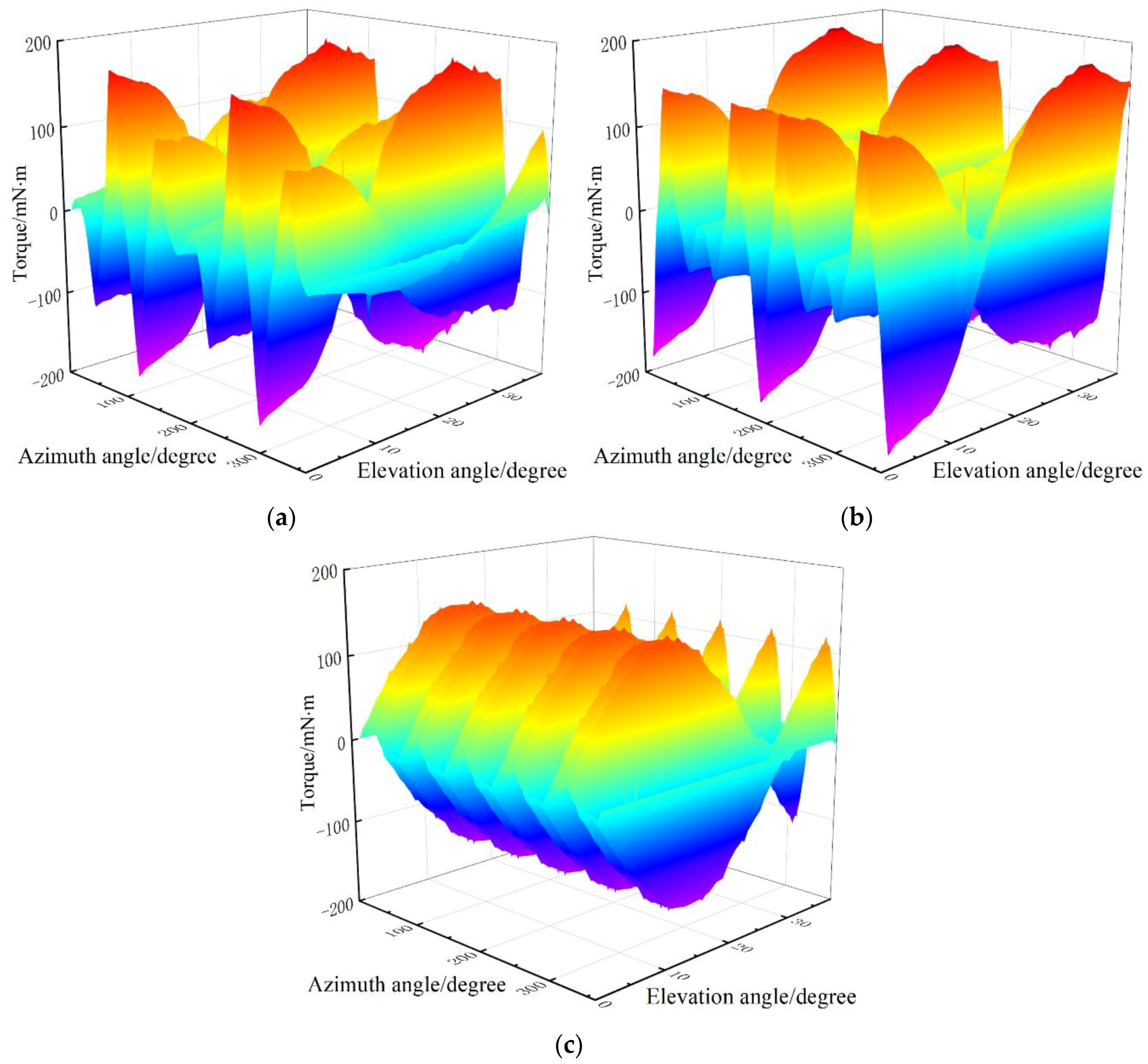
2.3. Torque Modeling

The establishment of the torque model can obtain the coil current through the rotor output torque. The PMs and coils on the PMSpA are symmetrically distributed in space. Since the stator adopts air-core coils, there is no saturation effect [27].

When the unit current flows into the stator coil, using the finite element method, the relationship between the relative position of the single stator coil and single PM and the generated electromagnetic torque can be obtained. Through the superposition principle, the torque model can be expressed as [28]:

$$u_{ij}={\displaystyle \sum _{i=1}^{40}{\displaystyle \sum _{j=1}^{24}f({\theta }_{ij})\frac{S_{ri}\times S_{rj}}{\left|S_{ri}\times S_{rj}\right|}{I}_i}},$$

(7)

where f(θ_ij) is the corresponding torque characteristic curve; θ_ij is the deflection angle; S_ri and S_rj are the position vectors of the coils and the PMs, respectively; and I_i is the coil current. Equation (7) can be converted into matrix form as follows:

$$u=\left[\begin{array}{c}{u}_x\\ u_y\\ u_z\end{array}\right]=\left[\begin{array}{cccc}{f}_{x1}& f_{x2}& \cdots & f_{x24}\\ f_{y1}& f_{y2}& \cdots & f_{y24}\\ f_{z1}& f_{z2}& \cdots & f_{z24}\end{array}\right]\cdot \left[\begin{array}{c}{I}_1\\ I_2\\ ⋮\\ I_{24}\end{array}\right]=f\cdot I,$$

(8)

where u_x, u_y, and u_z represent the spin torque, pitch torque, and yaw torque, respectively; and f_xi, f_yi, and f_zi are the torque components along three directions under the unit current (1A). The torque output map is shown in Figure 3. According to Equation (8), the current vector generating the required torque can be calculated by I = f^T (f f^T)⁻¹u.

3. Design of Controller

3.1. TDC Controller

Substitute Equation (6) into (5) to obtain the delay estimate value as follows:

$$Q{(\theta ,\dot{\theta },\ddot{\theta })}_{t-L}=u_{t-L}-\overline{N}{\ddot{\theta }}_{t-L}.$$

(9)

The control objective of TDC is the same as that of CTC, and the ideal dynamic error equation of the system is as follows:

$$\ddot{e}+K_d\dot{e}+K_{p}e=0,$$

(10)

where e = θ_d − θ represents PMSpA position tracking errors.

Combining Equations (5), (6), (9) and (10), the TDC output torque is obtained as follows:

$$\begin{array}{cc}\hfill u& =\overline{N}\ddot{\theta }+Q(\theta ,\dot{\theta },\ddot{\theta })=\overline{N}\ddot{\theta }+Q{(\theta ,\dot{\theta },\ddot{\theta })}_{t-L}=\overline{N}\ddot{\theta }+u_{t-L}-\overline{N}{\ddot{\theta }}_{t-L}\hfill \\ & =\overline{N}({\ddot{\theta }}_d-\ddot{e})+u_{t-L}-\overline{N}{\ddot{\theta }}_{t-L}=\overline{N}({\ddot{\theta }}_d+K_d\dot{e}+K_{p}e)+u_{t-L}-\overline{N}{\ddot{\theta }}_{t-L}\end{array}.$$

(11)

where ${\theta }_d={[{\alpha }_d,{\beta }_d,{\gamma }_d]}^T$ represents the expected Euler angle trajectory of the PMSpA; and K_p and K_d represent the diagonal gain matrix of the PD controller.

In practical applications, L represents the system sampling time, and its value will be restricted. The limitation of the value of L will cause the time delay estimation errors. From Equations (5), (6), (9) and (11), we can get

$$\begin{array}{cc}\hfill Q(\theta ,\dot{\theta },\ddot{\theta })-\widehat{Q}(\theta ,\dot{\theta },\ddot{\theta })& =Q(\theta ,\dot{\theta },\ddot{\theta })-Q{(\theta ,\dot{\theta },\ddot{\theta })}_{t-L}=Q(\theta ,\dot{\theta },\ddot{\theta })-(u_{t-L}-\overline{N}{\ddot{\theta }}_{t-L})\hfill \\ & =(u-\overline{N}\ddot{\theta })-[u-\overline{N}({\ddot{\theta }}_d+K_d\dot{e}+K_{p}e)]=\overline{N}(\ddot{e}+K_d\dot{e}+K_{p}e).\end{array}$$

(12)

From Equations (10)–(12), the time delay estimation errors λ can be obtained as

$$\lambda ={\overline{N}}^{-1}[Q(\theta ,\dot{\theta },\ddot{\theta })-Q{(\theta ,\dot{\theta },\ddot{\theta })}_{t-L}]=\ddot{e}+K_d\dot{e}+K_{p}e.$$

(13)

When there are nonlinear disturbances such as uncertainty, friction, and load torque, λ will become very large, which will affect the trajectory tracking effect.

3.2. TDC Controller with Gradient Compensation

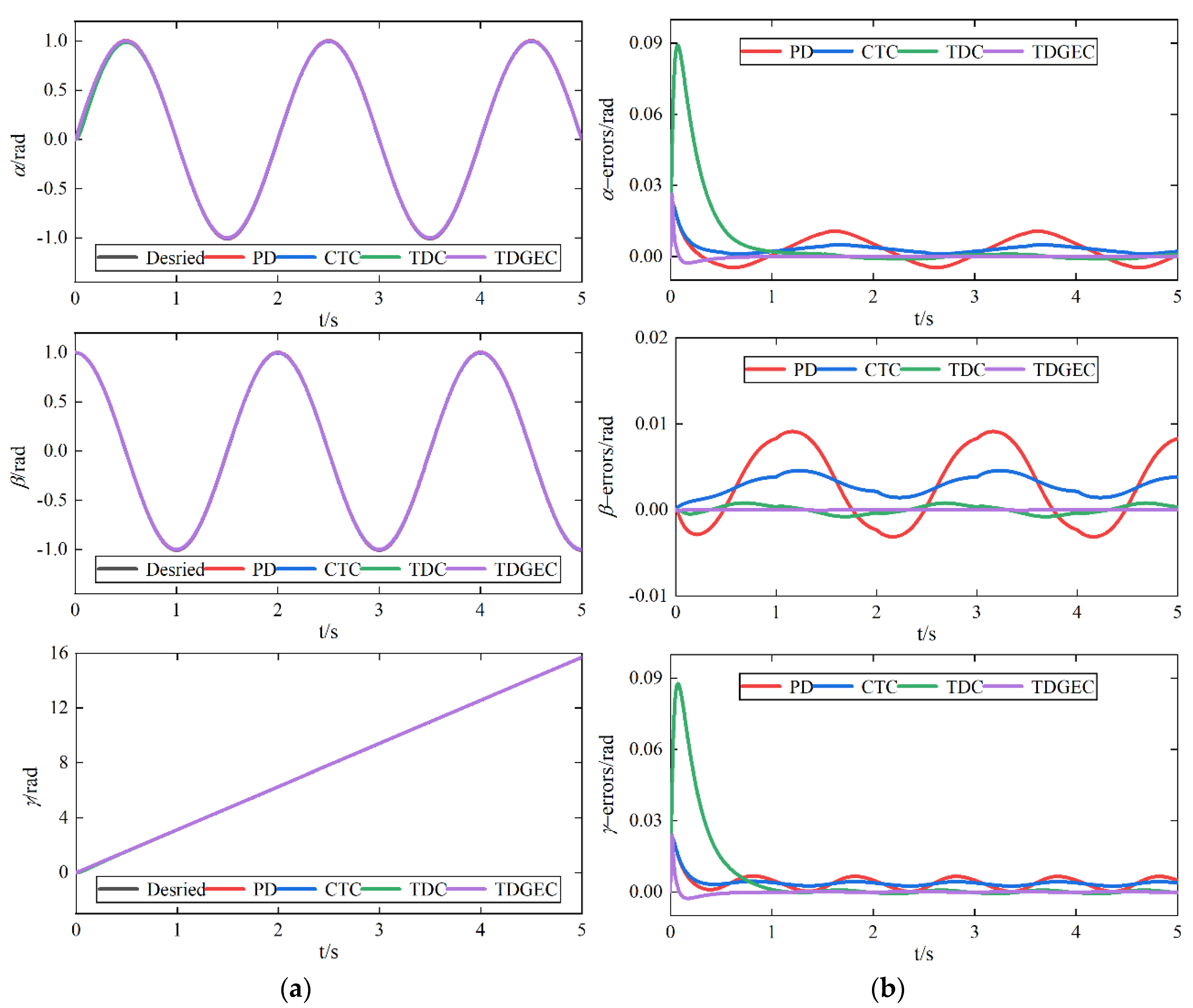
In order to suppress λ, this paper designs a time delay estimation controller with gradient compensation. The design process is as follows.

Firstly, the gradient compensation term $\widehat{\lambda }$ is introduced into Equation (11) to get:

$$u=u_{t-L}-\overline{N}{\ddot{\theta }}_{t-L}+\overline{N}({\ddot{\theta }}_d+K_d\dot{e}+K_{p}e)+\overline{N}\widehat{\lambda }.$$

(14)

With the combination of Equations (5) and (14), the dynamic error of the time delay estimation control system with gradient compensation is defined as follows:

$$\ddot{e}+K_d\dot{e}+K_{p}e=\lambda -\widehat{\lambda }=-\tilde{\lambda },$$

(15)

where $\tilde{\lambda }\stackrel{\Delta }{=}\widehat{\lambda }-\lambda$ represents the estimated error value of λ.

Secondly, the cost function of the λ is defined as

$$H(\tilde{\lambda })=\frac{1}{2}{\tilde{\lambda }}^T\tilde{\lambda }.$$

(16)

We used one assumption that the time delay estimation error λ is slow-varying or constant. The gradient compensator is designed as:

$$\dot{\widehat{\lambda }}=-K_{GC}\frac{\partial H}{\partial \widehat{\lambda }}=-K_{GC}\tilde{\lambda }=K_{GC}(\ddot{e}+K_d\dot{e}+K_{p}e),$$

(17)

where K_GC $\stackrel{\Delta }{=}$ diag(K_GC1, …, K_GCn) represents the gain matrix of the gradient compensator. The update of the gradient compensation amount can make the cost function Equation (16) always be negative, which can reduce λ.

The gradient compensation term $\widehat{\lambda }$ can be defined as

$$\widehat{\lambda }=K_{GC}(\dot{e}+K_{d}e+K_p{\displaystyle \int e}dt).$$

(18)

Therefore, Equation (14) is equivalent to

$$\begin{array}{cc}\hfill u& =u_{t-L}-\overline{N}{\ddot{\theta }}_{t-L}+\overline{N}({\ddot{\theta }}_d+K_d\dot{e}+K_{p}e)+\overline{N}\widehat{\lambda }\hfill \\ & =u_{t-L}-\overline{N}{\ddot{\theta }}_{t-L}+\overline{N}({\ddot{\theta }}_d+K_d\dot{e}+K_{p}e)+\overline{N}{K}_{GC}(\dot{e}+K_{d}e+K_p{\displaystyle \int e}dt)\end{array}.$$

(19)

It can be seen from Equation (19) that λ can be reduced by adjusting gain K_GC and does not require complete dynamic calculation. $K_{GC}{K}_p{\displaystyle \int e}dt$ in Equation (18) makes the effect of time delay estimation better, and only $\overline{N}$ and K_GC need to be adjusted in the entire control law, which is convenient for the actual controller design.

The trajectory tracking block diagram of the PMSpA system is shown in Figure 4.

In order to demonstrate the stability of the PMSpA control system based on gradient compensation, Theorem 1 is defined as follows (The proof of Theorem 1 is given in Appendix B):

Theorem 1.

Consider the PMSpA motion control system (2) with nonlinear disturbances and load, under the derived control law (19) with the time delay estimation (11) and gradient compensation term (18), the closed-loop system is gradually stable. The tracking error e is also uniformly bounded.

4. Simulations

In order to compare the simulation effect of the proposed controller, this paper designs four comparative control schemes: (1) the PD method; (2) the CTC method; (3) the TDC method; and (4) the proposed TDGEC method. According to Figure 4, a simulation model of the PMSpA position tracking control system is built in the MATLAB/SIMULINK environment, as shown in Figure 5. First, the given trajectory θ_d is input to the controller. According to the general design steps of the TDC controller, the error dynamics is injected into the TDGEC controller. At the same time, the error dynamics are passed through the gradient compensator to get $\widehat{\lambda }$, which can reduce the estimation error caused by the TDC. Finally, the actual control torque u is constructed by combining the output torque of the previous moment to drive the PMSpA for trajectory tracking control.

Under the same expected trajectory and nonlinear disturbance, Section 4.1 and Section 4.2 are designed for simulation under different modeling errors and different load torque, respectively.

The simulation parameters are set as follows. The control gains of the PD controller and CTC controller are both K_p = diag{30,30,30}, K_d = diag{5,5,5}. According to the actual size and structural parameters of the PMSpA prototype, the rotational inertia calculated using COMSOL Multiphysics^® is as follows:

$$\{\begin{array}{c}{I}_{dq}=1.548\times {10}^{-2}(kg\cdot m^2)\\ I_p=1.571\times {10}^{-2}(kg\cdot m^2)\end{array}.$$

(20)

To verify that the PMSpA has fully controllable operating conditions, the desired trajectory is set as

$${\theta }_d={[\begin{array}{ccc}\sin (\pi t)& \cos (\pi t)& \pi t\end{array}]}^T,t\in [0,5].$$

(21)

The initial position and speed setting of the system are as follows:

$$\{\begin{array}{c}{\theta }_d(0)={[\begin{array}{ccc}0& 1.0& 0\end{array}]}^T\hfill \\ {\dot{\theta }}_d(0)={[\begin{array}{ccc}0& 0& 0\end{array}]}^T\hfill \end{array}.$$

(22)

The modeling errors are set as:

$$\Delta J(\theta )+\Delta C(\theta ,\dot{\theta })=r\times [J(\theta )+C(\theta ,\dot{\theta })].$$

(23)

where r represents the modeling error coefficient.

The nonlinear disturbance F_q are set as the following two parts:

$$\{\begin{array}{c}{F}_{q1}=0.03\times {[\begin{array}{ccc}\sin (\pi t)& \cos (\pi t)& \exp (-0.5\pi t)\end{array}]}^T\hfill \\ F_{q2}=0.02\times sign(\dot{\theta })\hfill \end{array}.$$

(24)

The load torque is set as

$$d=w\times {[\begin{array}{ccc}0.15& 0.15& 0.15\end{array}]}^T.$$

(25)

where w is the load moment coefficient.

The sampling time L of the system is set to 0.001 s. The gain matrices of the TDC controller are $\overline{N}$ = diag{0.006,0.007,0.008}, K_p = diag{120,120,120}, K_d = diag{30,30,30}, and K_GC = diag{100,100,100}.

4.1. Simulation under Different Modeling Errors

In order to verify the influence of the modeling error on the proposed controller, it is assumed that the model has varying degrees of uncertainty. Based on the interference as shown in Equation (24), the load moment coefficient w and the modeling error coefficient r are set as 1 and 0.4, respectively, which means that the system has 40% modeling uncertainty. The tracking curves and tracking error curves of the four controllers are shown in Figure 6a,b, respectively.

It can be observed from Figure 6a that under the condition of 40% model uncertainty, the trajectory tracking using the TDGEC algorithm fits the desired trajectory well. In addition, the tracking error curves show that the error change of the system using the TDGEC algorithm is more stable. Under 40% modeling error, using four control algorithms, the absolute of the Max Steady-State Error (AMSSE) in three directions is shown in

Table 2. AMSSE values.

AMSSE (rad)	PD	CTC	TDC	TDGEC
α	0.0107	4.94 × 10−3	8.98 × 10−4	5.02 × 10−5
β	0.0091	4.56 × 10−3	7.85 × 10−4	2.82 × 10−5
γ	6.56 × 10−3	4.31 × 10−3	7.61 × 10−4	5.07 × 10−5

. The AMSSE values of using the TDGEC method are 5.02 × 10⁻⁵ rad, 2.82 × 10⁻⁵ rad, and 5.07 × 10⁻⁵ rad, which are much smaller than those of the other three controllers.

Furthermore, select the Root Mean Square Error (RMSE) under the four controllers to evaluate the adaptability and robustness of the controller. Figure 7 shows the RMSE with the variation of r from 0.2 to 0.8. The RMSE using the TDGEC controller is the smallest compared with the other three controllers. The results show that the TDGEC control method is not sensitive to the model parameters. In the presence of model uncertainty, the TDGEC controller can obtain better performance and better robustness.

4.2. Simulation under Different Load Torque

In the practical applications, the load will affect the control accuracy to a certain extent. In this section, the four controllers are designed with modeling error coefficient r = 0.3. The load torque coefficient w is changed from 1 to 5, which means that the system is under 30% model uncertainty and has to withstand different degrees of load torques. The parameter setting of the four controllers is the same as mentioned above. The tracking curves and tracking error curves when the load torque coefficient w = 3 are shown in Figure 8a,b, respectively.

Similarly, the AMSSE values under the four control methods are shown in

Table 3. AMSSE values.

AMSSE (rad)	PD	CTC	TDC	TDGEC
α	0.0161	0.0104	8.90 × 10−4	4.61 × 10−5
β	0.0146	0.0101	6.98 × 10−4	2.56 × 10−5
γ	0.0123	0.0101	7.06 × 10−4	4.71 × 10−5

. The expected trajectory is closely tracked using the TDGEC controller, which can be seen in Figure 8a. In addition, we can see from Figure 8b that under PD control and CTC control, the steady-state tracking error is very obvious, which means that the load seriously affects the tracking accuracy. In contrast, the tracking error after reaching the steady-state is the smallest with the TDGEC controller, and the AMSSE values are only 4.61 × 10⁻⁵ rad, 2.56 × 10⁻⁵ rad, and 4.71 × 10⁻⁵ rad, respectively.

Figure 9 shows the RMSE when w varies from 1 to 5. It can be seen that with the change of w, the RMSE of the TDGEC controller is the smallest among the four control methods. Moreover, the RMSE value has no noticeable change. However, when the load changes with the PD controller and CTC controller, the RMSE value changes obviously, indicating that the robustness of these two controllers is poor. The simulation results demonstrate that the TDGEC controller can maintain a good tracking effect under the influence of the external load torque.

From the above numerical simulation results, we can conclude that the proposed TDGEC controller offers an improved controller design for high-precision motion control of PMSpA with model uncertainty and nonlinear disturbances. Furthermore, the control gain adjustment is simple, which is convenient for the actual controller design.

5. Experiment Evaluation

5.1. Experimental Platform and Principle

The experimental platform is shown in Figure 10. The experimental platform includes a host computer, a PMSpA prototype, the current driver, a MEMS sensor, and a power supply. The rotor output shaft is equipped with a flange to transmit the electromagnetic torque generated by the actuator. Communication between the host computer and the current driver is through the serial port.

As shown in Figure 11, the upper computer obtains the position information from the MEMS sensor and executes the control algorithm. A graphical user interface program is written on the host computer. Through this interface, the user can easily adjust the control parameters, set the desired trajectory, and send the current command. The user can also observe the attitude information of the output shaft in real time on this interface. The MEMS sensor can obtain the position information of the output shaft in time and send it to the upper computer through the Bluetooth device. Then the control torque is obtained according to the control law Equation (19). The current reference values of the 24 stator coils are solved according to the torque model in Section 2.3, which are sent to the current driver through the RS485 serial port.

The current driver includes 24 individual driving units, each containing an ARM processor. The driving unit is powered by 24 V DC power supply and uses power transistors 2SC4552 to adjust the current of 24 stator coils in the form of the controllable constant current source. In addition, the main circuit of the driving units consists of a single-phase H-bridge, a power transistor connected in series with it and a sampling resistor. The H-bridge is composed of two P-MOSFETs and two N-MOSFETs. The single-phase H-bridge circuit controls the direction of the current flowing through the stator coil. After receiving the current command from the host computer, it provides current to 24 stator coils to generate the electromagnetic torque, thereby driving the PMSpA movement.

5.2. Experiment and Analysis

Two simple tracking trajectories are set up in the experiment to observe the control performance of the proposed controller, as shown below:

$${\theta }_{d1}={[\begin{array}{ccc}\alpha (t)& 0& 0\end{array}]}^T,$$

(26)

$${\theta }_{d2}={[\begin{array}{ccc}0& \beta (t)& 0\end{array}]}^T,$$

(27)

where $\alpha (t),\beta (t)=\{\begin{array}{l}0.5t,t\in [0,20]\\ 10,t\in [20,30]\end{array}$.

In the experiment, the PD controller and TDC controller are used to compare with the TDGEC controller. Three controllers’ parameter setting is shown in

Table 4. Parameter setting of three controllers.

	PD	TDC	TDGEC
Kp	diag{0.02,0.02,0.02}	diag{0.05,0.05,0.05}	diag{0.05,0.05,0.05}
Kd	diag{0.005,0.005,0.005}	diag{0.02,0.02,0.02}	diag{0.02,0.02,0.02}
$\overline{N}$	-	diag{0.003,0.004,0.004}	diag{0.003,0.004,0.004}
KGC	-	-	diag{0.08,0.08,0.08}

, and the trajectory tracking curves are shown in Figure 12a,b.

As we can see from Figure 12, the actual tracking trajectory is closer to the expected trajectory, and the rising phase is more stable with the TDGEC controller. When the PD controller is used, the trajectory is stepped. In addition, the error from the expected trajectory after reaching stability is obviously greater than that of the TDGEC controller. Furthermore, the tracking errors are statistically analyzed, and the steady-state error (SSE), the absolute value of maximum of error (AME), and the standard deviation of error are shown in

Table 5. The SSE, AME, and the standard deviation.

	PD		TDC		TDGEC
	α	β	α	β	α	β
SSE (degree)	0.814	0.714	0.614	0.494	0.414	0.246
AME (degree)	1.869	1.635	1.449	1.247	0.743	0.799
Standard deviation (degree)	0.487	0.327	0.590	0.532	0.319	0.240

.

From the statistical results, the SSE in α and β using PD controller and TDC controller are 0.814°, 0.714° and 0.614°, 0.494°, respectively. While using the TDGEC controller, the SSE are only 0.414° and 0.246°. The AME or the standard deviation of the TDGEC controller is smaller than that of the PD controller and CTC controller. It is worth noting that the traditional TDC control will increase the standard deviation, which means that the error fluctuation is greater. In contrast, the TDGEC control can effectively reduce the standard deviation by about 45% and reduce the error fluctuation.

6. Conclusions

Based on the TDC control algorithm, this paper uses gradient compensation to reduce the estimation errors caused by TDC control. There are uncertainties and various external interferences in the dynamic model of the PMSpA. In this situation, the proposed method still has a good trajectory tracking effect. Both simulation and experiment have also shown that the TDGEC controller has high tracking accuracy, good robustness to system model uncertainty and load disturbance, and can effectively reduce the estimation error caused by the TDC controller. In addition, it has a simple structure and simple control gain adjustment. It lays the foundation for the industrial applications of the spherical motors.

References

1. Yang, L.; Chen, I.M.; Lim, C.K.; Yang, G.; Lin, W.; Lee, K.M. Design and analysis of a permanent magnet spherical actuator. IEEE-ASME Trans. Mechatron. 2008, 13, 239–248. [Google Scholar] [CrossRef]
2. Wright, S.E.; Mahoney, A.W.; Popek, K.M.; Abbott, J.J. The Spherical-Actuator-Magnet Manipulator: A Permanent-Magnet Robotic End-Effector. IEEE Trans. Robot. 2017, 33, 1013–1024. [Google Scholar] [CrossRef]
3. Li, Z.; Gao, S.H.; Zhang, H.M. Wireless power transmission for multi-degree-of-freedom motor applications based on magnetic field coupling. IEICE Electron. Express. 2019, 16, 20190330. [Google Scholar] [CrossRef]
4. Fernandes, J.F.P.; Branco, P.J.C. The Shell-Like Spherical Induction Motor for Low-Speed Traction: Electromagnetic Design, Analysis, and Experimental Tests. IEEE Trans. Ind. Electron. 2016, 63, 4325–4335. [Google Scholar] [CrossRef]
5. Bai, K.; Xu, R.Y.; Lee, K.M.; Dai, W.; Huang, Y.A. Design and Development of a Spherical Motor for Conformal Printing of Curved Electronics. IEEE Trans. Ind. Electron. 2018, 65, 9190–9200. [Google Scholar] [CrossRef]
6. Maeda, S.; Hirata, K.; Niguchi, N. Dynamic Analysis of an Independently Controllable Electromagnetic Spherical Actuator. IEEE Trans. Magn. 2013, 49, 2263–2266. [Google Scholar] [CrossRef]
7. Yan, L.; Wu, Z.W.; Jiao, Z.X.; Chen, C.Y.; Chen, I.M. Equivalent energized coil model for magnetic field of permanent-magnet spherical actuators. Sens. Actuator A Phys. 2015, 229, 68–76. [Google Scholar] [CrossRef]
8. VanNinhuijs, B.; Motoasca, T.E.; Gysen, B.L.J.; Lomonova, E.A. Modeling of Spherical Magnet Arrays Using the Magnetic Charge Model. IEEE Trans. Magn. 2013, 49, 4109–4112. [Google Scholar] [CrossRef]
9. Son, H.S.; Lee, K.M. Open-Loop Controller Design and Dynamic Characteristics of a Spherical Wheel Motor. IEEE Trans. Ind. Electron. 2010, 57, 3475–3482. [Google Scholar] [CrossRef]
10. Son, H.S.; Lee, K.M. Control system design and input shape for orientation of spherical wheel motor. Control. Eng. Pract. 2014, 24, 120–128. [Google Scholar] [CrossRef]
11. Chen, W.H.; Zhang, L.; Yan, L.; Liu, J.M. Design and control of a three degree-of-freedom permanent magnet spherical actuator. Sens. Actuator A Phys. 2012, 180, 75–86. [Google Scholar] [CrossRef]
12. Zhang, L.; Chen, W.H.; Liu, J.M.; Wen, C.Y. A Robust Adaptive Iterative Learning Control for Trajectory Tracking of Permanent-Magnet Spherical Actuator. IEEE Trans. Ind. Electron. 2015, 63, 291–301. [Google Scholar] [CrossRef]
13. Nguyen, K.D. On the adaptive control of spherical actuators. Trans. Inst. Meas. Control. 2019, 41, 816–827. [Google Scholar] [CrossRef]
14. Xia, C.L.; Guo, C.; Shi, T.N. A Neural-Network-Identifier and Fuzzy-Controller-Based Algorithm for Dynamic Decoupling Control of Permanent-Magnet Spherical Motor. IEEE Trans. Ind. Electron. 2010, 57, 2868–2878. [Google Scholar] [CrossRef]
15. Guo, X.W.; Pan, K.D.; Wang, Q.J.; Wen, Y. Robust Adaptive Sliding-Mode Control of a Permanent Magnetic Spherical Actuator with Delay Compensation. IEEE Access 2020, 8, 128096–128105. [Google Scholar] [CrossRef]
16. Yan, L.; Zhang, L.; Zhu, B.; Zhang, J.Y.; Jiao, Z.X. Single neural adaptive controller and neural network identifier based on PSO algorithm for spherical actuators with 3D magnet array. Rev. Sci. Instrum. 2017, 88, 105001. [Google Scholar] [CrossRef] [PubMed]
17. Youcef, T.K.; Ito, O. A Time Delay Controller for Systems with Unknown Dynamics. J. Dyn. Syst. Meas., Control. 1990, 112, 133–142. [Google Scholar] [CrossRef]
18. Chang, P.H.; Park, S.H. On improving time-delay control under certain hard nonlinearities. Mechatronics 2003, 13, 393–412. [Google Scholar] [CrossRef]
19. Jin, M.L.; Kang, S.H.; Chang, P.H. Robust Compliant Motion Control of Robot with Nonlinear Friction Using Time-Delay Estimation. IEEE Trans. Ind. Electron. 2008, 55, 258–269. [Google Scholar] [CrossRef]
20. Baek, J.; Jin, M.; Han, S. A New Adaptive Sliding-Mode Control Scheme for Application to Robot Manipulators. IEEE Trans. Ind. Electron. 2016, 63, 3628–3637. [Google Scholar] [CrossRef]
21. Baek, J.; Kwon, W.; Kim, B.; Han, S. A Widely Adaptive Time-Delayed Control and Its Application to Robot Manipulators. IEEE Trans. Ind. Electron. 2019, 66, 5332–5342. [Google Scholar] [CrossRef]
22. Jin, M.L.; Kang, S.H.; Chang, P.H.; Lee, J. Robust Control of Robot Manipulators Using Inclusive and Enhanced Time Delay Control. IEEE-ASME Trans. Mechatron. 2017, 22, 2141–2152. [Google Scholar] [CrossRef]
23. Jiang, S.R.; Wang, Y.Y.; Ju, F.; Chen, B.; Wu, H.T. A new fuzzy time-delay control for cable-driven robot. Int. J. Adv. Robot. Syst. 2019, 16, 1729881419835017. [Google Scholar] [CrossRef] [Green Version]
24. Wang, J.; Jewell, G.W.; Howe, D. Analysis, design and control of a novel spherical permanent-magnet actuator. IEE Proc.—Electr. Power Appl. 1998, 145, 61–71. [Google Scholar] [CrossRef]
25. Li, H.L.; Li, G.L.; Wang, Q.J.; Ju, B.; Wen, Y. Friction torque field distribution of a permanent-magnet spherical motor based on multi-physical field coupling analysis. IET Electr. Power Appl. 2021, 15, 1045–1055. [Google Scholar] [CrossRef]
26. Lee, K.M.; Vachtsevanos, G.; Kwan, C. Development of a spherical stepper wrist motor. J. Intell. Rob. Syst. 1988, 1, 225–242. [Google Scholar] [CrossRef]
27. Xia, C.L.; Li, H.F.; Shi, T.N. 3-D magnetic feld and torque analysis of a novel Halbach array permanent-magnet spherical motor. IEEE Trans. Magn. 2008, 44, 2016–2020. [Google Scholar] [CrossRef]
28. Wen, Y.; Li, G.L.; Wang, Q.J.; Guo, X.W. Robust Adaptive Sliding-Mode Control for Permanent Magnet Spherical Actuator with Uncertainty Using Dynamic Surface Approach. J. Electr. Eng. Technol. 2019, 14, 2341–2353. [Google Scholar] [CrossRef]
29. Hsia, T.C.; Gao, L.S. Robot manipulator control using decentralized linear time-invariant time-delayed joint controllers. In Proceedings of the IEEE International Conference on Robotics and Automation, Cincinnati, OH, USA, 13–18 May 1990; pp. 2070–2075. [Google Scholar] [CrossRef]
Figure 1. PMSpA structure diagram.
Electronics 11 00066 g001
Figure 2. Movement diagram.
Electronics 11 00066 g002
Figure 3. The torque map of the PMSpA: (a)Spinning torque, (b) Pitching torque, and (c) Yawing torque.
Electronics 11 00066 g003
Figure 4. Controller system block diagram: (a) Feedforward function processing, (b) PD-type feedback, (c) Time delay estimation, and (d) Gradient compensator.
Electronics 11 00066 g004
Figure 5. Simulink model.
Electronics 11 00066 g005
Figure 6. Simulation results: (a) Tracking curves (r = 0.4) and (b) Tracking error curves (r = 0.4).
Electronics 11 00066 g006
Figure 7. RMSE under different r.
Electronics 11 00066 g007
Figure 8. Simulation results: (a) Tracking curves (w = 3) and (b) Tracking error curves (w = 3).
Electronics 11 00066 g008
Figure 9. RMSE under different w.
Electronics 11 00066 g009
Figure 10. The experiment platform.
Electronics 11 00066 g010
Figure 11. The principle of experimental operation.
Electronics 11 00066 g011
Figure 12. Trajectory tracking curves: (a) α-axis tracking trajectory and (b) β-axis tracking trajectory.
Electronics 11 00066 g012