Abstract
Aiming at the influence of friction, leakage, noise and other nonlinear factors on the performance of the electro-hydraulic servo system of a continuous rotary motor, a finite-time composite controller for the aforementioned servo system is proposed. First, a mathematical model of the electro-hydraulic servo system was analyzed, and the input and output angle data of the motor were collected for system identification. Subsequently, the ARMAX identification model of the continuous rotary motor system was obtained. Then, according to the observed advantages, namely faster capability of the finite-time controller (FTC) to converge the system, and ability of the finite-time observer to reduce the steady-state error of the system, the finite-time controller and finite-time state observer of a continuous rotary electro-hydraulic servo motor were respectively designed. Finally, comparison with PID control simulation shows that the compound controller could effectively improve the control accuracy and performance of the system.
1. Introduction
The continuous rotary electro-hydraulic servo motor represents the core instrument in driving the hydraulic simulation turntable. The interference of oil-source pulsation, friction, leakage and uncertain external factors in the system, makes it difficult to establish an accurate mathematical model [,,], that is unable to meet the control performance requirements of continuous rotary electro-hydraulic servo motor systems. Thus, to enhance electro-hydraulic servo motor performance, it is necessary to establish both a more accurate model of the servo system and a more reasonable controller design that can withstand the poorest of conditions. This challenge has become one of the main hotspots in research [,,].
Aiming at the problems of nonlinear disturbance and parameter change in the electro-hydraulic servo system, an adaptive fuzzy PID controller with online parameter adjustment was designed in reference []. The researchers experimentally verified the effectiveness of the controller, which was of great significance in improving the position control accuracy of the parallel motion platform. In reference [], the adaptive back stepping sliding mode control algorithm was proposed in order to solve issues regarding external disturbances on the system. Experiments showed that the controller had strong robustness and could well realize the position control of the electro-hydraulic servo system. In reference [], in order to solve the uncertainty of the system and the disturbance caused by friction torque, QFT (Quantitative Feedback Control) was applied to the motor position control system; however, the influence of leakage was not considered. In reference [], in order to improve the position control precision of the branch chain of a parallel moving platform, the adaptive inverse sliding mode control algorithm was proposed. This proposal aimed to solve the influence of external disturbances on the position control system of the parallel moving platform and its branch chain. The experimental results revealed strong robustness of the controller. To enhance the performance of PMSM and to reduce the influence of parameter perturbation and other factors on the system, a nonlinear position tracker was designed in reference [], and the finite-time stability of the controller was proven. In reference [], the background, basic definition and judgment method of finite-time control were described, and the control problems and controller design were thoroughly investigated. In reference [], according to neural network, sliding mode control theory and control allocation technology, a finite-time composite control strategy was proposed for the attitude control of an aerospace vehicle in the loading phase. The effectiveness of the proposed control strategy was verified by simulation. In reference [], a non-smooth compound controller was designed to study the third-order saturated nonlinear system. On the premise that the initial conditions of the system were known, the system state gradually approached the equilibrium point. Simulation results showed that the algorithm could improve the performance of the system. In reference [], the problem of non-smooth optimal control was studied, and the sufficient optimality conditions with or without Lagrange multiplier were given, respectively. In reference [], a non-smooth finite-time control method was proposed to control the wheel steering angle, and the performance of the controller was experimentally verified. In reference [], an adaptive continuous non-smooth partial-state feedback controller without hyper-parameterization was designed, and the effectiveness of the method was demonstrated by simulation. In reference [], a compound controller was designed to eliminate the influence of disturbances on a permanent-magnet synchronous motor. Through simulation and experimentation, it was subsequently demonstrated that the controller could eliminate the influence of disturbances on the motor system.
The finite-time control exhibits fast convergence and robustness and the motor system is a nonlinear system with external interference. Therefore, employing the finite-time control can effectively improve the performance of the motor. In order to improve the continuous rotary motor electro-hydraulic servo system regarding better anti-interference ability and convergence speed enhancement of the motor system, the finite-time controller and finite-time state observer were employed to control the motor system on the basis of system model identification. The finite-time controller was designed to improve the convergence speed of the system, and the finite-time state observer was used to observe the state of the system. The simulation results show that the controller is feasible for the motor system and can improve system performance.
2. Transfer Function of Continuous Rotary Motor System
The schematic figure of the motor system is shown in Figure 1a. Oil is supplied by the plunger pump, and then the motor is controlled by the electro-hydraulic servo valve. When the motor begins operating, the hydraulic oil enters the oil inlet cavity 1 and 2 of the oil distribution plate through the electro-hydraulic servo valve to promote rotation of the motor blade. As the blade runs through the stator working area, the pressure of the relief valve is adjusted to make the blade root enter the oil, as to balance the liquid pressure on top of the blade. It is important to ensure that the motor blades maintain constant contact with the inner wall of the stator to form a sealed cavity. When the blade runs to the curve transition section in the stator, the oil in the oil chamber at the root of the blade and the oil in the working chamber at the top are connected with a specific flow distribution mechanism to prevent flow pulsation and to reduce friction between the blade and the stator.
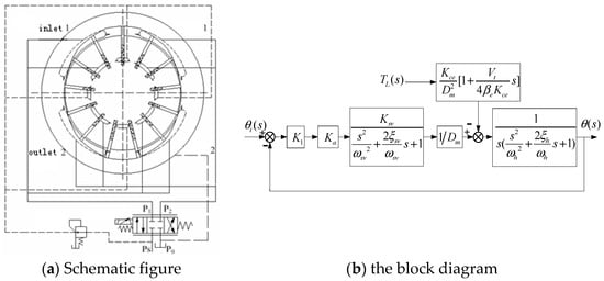
Figure 1.
A schematic figure and transfer function block diagram of the motor system.
2.1. Valve Port Flow Equation of Servo Valve
The linearized flow equation of the valve port of the electro-hydraulic servo valve is established, and the Laplace transform is as follows
where, QL is the load flow of motor (m3/s), Kq is the flow gain of electro-hydraulic servo valve port (m2/s), xv is the displacement of servo valve core (m), Kc is the flow pressure coefficient of servo valve port (m3/(s · Pa)), and PL is the load pressure (Pa).
2.2. Load Flow Continuity Equation of Motor
The load flow of the motor in working state consists of three parts: the flow required by normal continuous rotation of the motor, the internal and external leakage loss caused by friction and external interference, and the additional flow generated by oil compression. Through Laplace transform, the following equation can be obtained.
where, Dm is the arc displacement of the hydraulic motor (m3/rad), θ is the angular displacement of the hydraulic motor (rad), Ctm is the total leakage coefficient of the hydraulic motor (m3/(s · Pa)), Vt is the total volume of the hydraulic motor, servo valve cavity and connecting pipeline (m3), and βe is the effective bulk modulus of elasticity (Pa) of the working oil.
2.3. Motor Torque Balance Equation
Ignoring the influence of nonlinear load factors such as static friction force, based on Newton’s second law, the torque balance equation of the sum of motor torxes and load is established, which can be written by Laplace transform.
where, Jt is the total moment of inertia of the motor and external load (kg·m2), Bm is the viscous damping coefficient (N · m/(rad/s)), G is the spring stiffness of the load (N · m/rad), and TL is the load torque on the motor (N · m).
2.4. Transfer Function of Valve Controlled Motor Power Mechanism
According to Equations (1)–(3), the total output angular displacement xv(s) of the motor under the simultaneous action of spool displacement xv(s) and interference TL(s) can be obtained as follows.
where, Kce is the total flow pressure coefficient of valve controlled motor (m3/(s · Pa)).
In the connections of the hydraulic system, the motor and load are closely connected, so the influence of load stiffness is ignored. In other words, Equation (4) is usually simplified as follows.
where is the hydraulic natural frequency (rad/s), is the hydraulic damping ratio (dimensionless), .
If the no-load flow of the servo motor is Q0 = Kqxv, the transfer function of the motor output angular displacement to the no-load flow of the servo valve can be obtained from Equation (5).
2.5. Transfer Function of Servo Amplifier
Usually, the frequency of the servo amplifier is much higher than the natural frequency of the hydraulic system, so it is simplified as a proportional link.
where, Ka is gain of amplifier (A/V).
2.6. Transfer Function of Electro-Hydraulic Servo Valve
The transfer function of the electro-hydraulic servo valve is as follows.
where Ksv is no-load flow gain of servo valve (m3/(s · A)), ωsv is equivalent undamped natural frequency of servo valve (rad/s), and ξsv is the equivalent damping coefficient of the servo valve.
2.7. System Transfer Function of Continuous Rotary Electro-Hydraulic Servo Motor
The block diagram of the motor system is shown in Figure 1b, K1 is the transfer function of the main controller.
The open-loop transfer function of the motor system can be obtained from Figure 1b.
where, K is the open-loop gain of the system, .
3. Parameter Identification of Continuous Rotary Motor System
The initial frequency of the system input signal is 0.2 Hz, the peak to peak value is 2° and the frequency of the sweep signal increases by 0.2 Hz every four cycles. There is the ARX model, ARMAX model, OE model, BJ model and state space model. In this paper, the ARMAX discrete identification model is selected, which has the characteristics of strong flexibility, strong anti-noise ability, and considers the influence of other variables [].
After the identification data are processed, the first 80 s identification data are used for system identification, and the last 20 s data are used as model validation data. The identification results are as follows.
According to the identification data, the identification results of the continuous rotary motor system are compared as shown in Figure 2. The fitting degree between the identification results and the system identification output results is 87.76%. The same frequency sweeping signal is used for frequency sweeping of the identified system, and the result of frequency sweeping is compared with the actual identification result. A comparison diagram of the frequency sweeping result and identification result is shown in Figure 3. After calculation, the fitting degree between the frequency sweeping output and identification output is 71.35%. Because the fitting degree between the frequency sweep output and the identification output is more than 70%, the third-order model of identification is considered to be feasible.
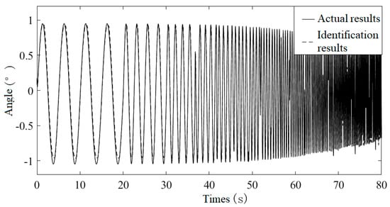
Figure 2.
Comparison of identification results.
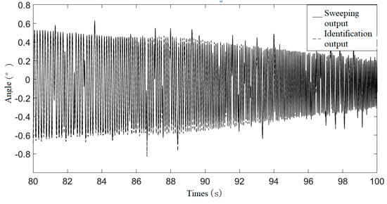
Figure 3.
Comparison diagram of verification section.
According to the identification results, the space state model of the motor system is established.
where, is the state of the system, is the rotation angle of the motor, is the angular velocity of the motor, is the angular acceleration of the motor, u is the output of the controller or the input of the motor system, and A, B, C and D are the motor parameter matrix.
4. Finite-Time Compound Control of Continuous Rotary Motor System
In order to study the performance of the continuous rotary motor electro-hydraulic servo system and improve the convergence speed of the motor system, the finite-time controller and the finite-time state observer are designed for the composite control of the motor system. The control strategy diagram is shown as Figure 4.
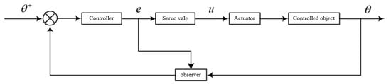
Figure 4.
Finite-time compound control flow chart of the continuous rotary motor system.
4.1. Finite-time Controller Structure
For the system satisfying the condition in reference [], the finite-time controller of the motor system is designed by using the power integral method and the step-by-step recursive method.
Step one: consider the first-order system of continuous rotary motor.
By selecting the Lyapunov function , the derivative of the system (12) is obtained.
Let be regarded as a virtual control law, and let be a virtual control law.
where, is an appropriate normal number, , .
Substituting Equation (14) into Equation (13), the following equation can be obtained.
The second step is to construct the Lyapunov function for the second-order system of the continuous rotary motor.
where, .
The derivative of Equation (15) gives the following equation.
where, is the appropriate normal number. According to Equation (16), it can be concluded that:
The virtual control law is set up as follows.
Substituting Equation (18) into Equation (17),
The third step is to design the finite-time controller. Lyapunov function is constructed as follows.
where,
It can be obtained by deriving along the Equation (19).
Making , then,
According to reference [], it can be seen that there is a derivable function.
According to reference [] and integrating the above formula.
where, is an appropriate normal number.
Let the control law be , e is the input and output error of the system, which can be obtained by substituting it into Equation (20).
The existence constants c2 and k3 satisfy , therefore,
Based on the properties of integral, the following inequality holds as follows.
It is not difficult to prove that is always true for . By synthesizing Equations (21) and (22), the follow formula can be obtained.
It can be seen from reference [] that the motor system is finite-time stable under the action of control law u. In summary, the finite-time controller is designed as follows.
4.2. Structure Design of Finite-time Observer
The motor system is a real-time changing system, which needs to observe the state variables. Therefore, the state variables are estimated through a model using the known information. The output u of the controller and the output θ of the motor system are used as the inputs of the state observer.
where, L1, L2 and L3 are appropriate constants,
It is assumed that there is a constant ,, therefore,
Definition and can be obtained from Equations (25) and (26).
where, .
In order to make the finite-time observer of the motor system converge, it is necessary to prove the existence of gain matrix L, which makes the system (27) converge in finite-time.
It can be seen from reference [] that there is a Lyapunov function with a degree of homogeneity of 2. By deriving the Lyapunov function along the system (27), it can be concluded as follows.
According to literature [], the following inequality can be obtained
According to the hypothesis in reference [], it can be concluded as follows.
From Equation (2),
where is an appropriate positive number. According to Equation (27), it can be concluded as follows.
Because there is a constant ,
In combination with reference [], there is a constant μ.
In combination with Equations (25) and (27), it can be obtained as follows.
It can be seen from the above equation that the system converges in finite-time.
4.3. Simulation of Finite-Time Compound Controller for Continuous Rotary Motor System
The finite-time compound control block diagram and PID control block diagram of motor system are built in Simulink, as shown in Figure 5. In order to improve the performance of the composite controller, the parameters of the controller and the observer are adjusted by the “separation principle” according to the setting rules.
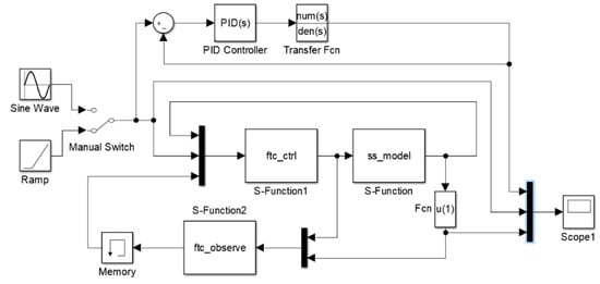
Figure 5.
Simulation diagram of finite-time compound control for the continuous rotary motor.
Finite-time controller part: parameter directly affects the stability time of the system, when is larger, the stability time of the system is shorter. When is small, the system oscillates easily, parameters k1, k2 and k3 are similar to P control, and appropriate k1, k2 and k3 can effectively improve the tracking accuracy of the system and reduce the static error of the system. In this paper, the parameters of finite-time controller are: = −0.001, k1 = 300, k2 = 186, k3 = 25.
Finite-time observer part: parameter is related to the stability of the observer . Increasing the tracking performance of the system and decreasing the tracking time will increase the stability time of the system. The value of each parameter in this paper is .
4.3.1. Slope Signal Simulation
The slope signal with 0.001°/s is used as the input signal to obtain the comparison diagram of the simulation results between the finite-time composite controller and the PID controller, as shown in Figure 6. In the figure, the solid line represents the ramp input signal, the dotted line represents the output curve of the system under the action of the PID controller, and the red dotted line represents the output curve of the system under the action of the finite-time compound controller. As can be seen from Figure 6, under the action of PID controller, the response time of the system is long and the response speed is slow. Under the action of finite-time compound control, the response speed of the system is fast, the tracking time is short, but there is a certain static error. Through the simulation of slope signal, both controllers can achieve the desired low speed performance of the system.
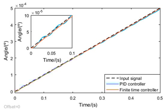
Figure 6.
Simulation diagram of finite-time composite control slope signal of the motor system.
4.3.2. Sinusoidal Signal Simulation
The motor system is simulated with a sinusoidal signal whose amplitude is 1° and frequency gradually increases, and the output comparison curves of finite-time composite control and PID control are obtained as shown in Figure 7, Figure 8, Figure 9, Figure 10, Figure 11, Figure 12 and Figure 13, where (a) is the sinusoidal response curve and (b) is the single periodic response curve. The solid line is the sinusoidal input signal at different frequencies, the dotted line is the output curve under the action of finite-time compound control, and the red dotted line is the output curve under the action of PID. Double ten index is used to measure whether the controller is effective, that is, compared with the input signal, the amplitude deviation of the output signal of the system is less than 10%, and the phase lag angle is less than 10°. Through the sinusoidal signal simulation of the motor system, the system tracking performance is shown in Table 1.
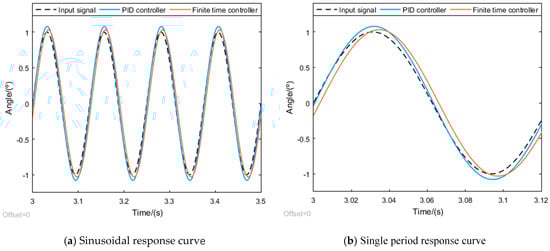
Figure 7.
Finite-time composite control response curve of the motor system with 8 Hz and 1° sinusoidal signal.
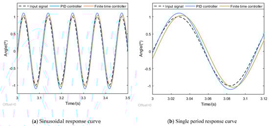
Figure 8.
Finite-time composite control response curve of the motor system with 9 Hz and 1° sinusoidal signal.
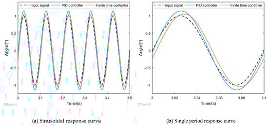
Figure 9.
Finite-time composite control response curve of the motor system with 10 Hz and 1° sinusoidal signal.
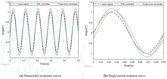
Figure 10.
Finite-time composite control response curve of the motor system with 11 Hz and 1° sinusoidal signal.
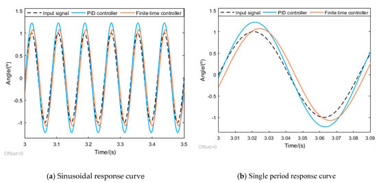
Figure 11.
Finite-time composite control response curve of the motor system with 12 Hz and 1° sinusoidal signal.
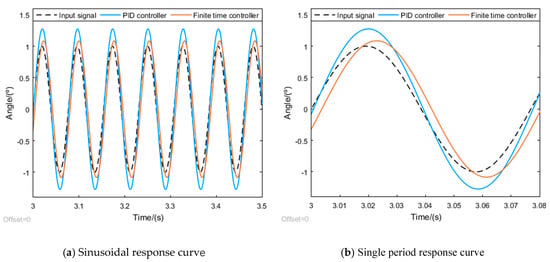
Figure 12.
Finite-time composite control response curve of the motor system with 13 Hz and 1° sinusoidal signal.
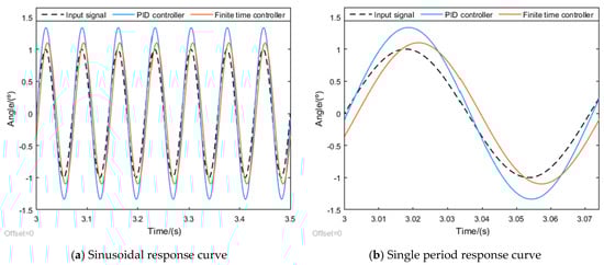
Figure 13.
Finite-time composite control response curve of the motor system with 14 Hz and 1° sinusoidal signal.

Table 1.
Comparison chart of system performance with 1° amplitude.
It can be seen from Table 1 that with the increase of input signal frequency, the amplitude error and phase error of the system increase much faster than the phase lag under PID controller. Under the action of finite-time composite controller, the amplitude error and phase error of the system increases slowly, and the phase error is greater than PID control. According to the data in the Table 1, PID controller only meets the double ten index when the sine frequency is 8 Hz, while the response frequency of the finite-time composite controller can reach 14 Hz, which proves that the performance of the finite-time composite control is better than that of the PID control. To sum up, the finite-time composite controller broadens the frequency band of the system, and its control performance is better than PID control.
5. Conclusions
In this paper, the finite-time composite controller of a continuous rotary motor electro-hydraulic servo system is designed. Firstly, the mathematical model of continuous rotary motor system is established, then the identification model of a continuous rotary electro-hydraulic servo system is obtained, and finally the finite-time composite controller is designed to control a continuous rotary electro-hydraulic servo system. By using the slope signal of 0.001°/s and sinusoidal signal with a different frequency as the input signal to control the system, the simulation comparison with PID control shows that the finite-time composite control can improve the low-speed performance of the system, broaden the frequency band and effectively improve the performance of the system. The system response frequency of the finite-time composite controller can reach 14 Hz, and the lowest stable speed of the motor system is 0.001°/s. In future research, the finite-time composite controller can be used for the actual motor system where the experimental conditions are permitted, and the controller effect can be further verified.
Author Contributions
Conceptualization, X.-J.W.; methodology, C.-H.L.; software, Q.-Z.Z.; validation, X.-J.W., Q.-Z.Z. and C.-H.L.; formal analysis, C.-H.L.; investigation, Q.-Z.Z.; resources, X.-J.W.; data curation, C.-H.L.; writing—original draft preparation, Q.-Z.Z.; writing—review and editing, X.-J.W.; visualization, C.-H.L.; supervision, X.-J.W.; project administration, X.-J.W.; funding acquisition, X.-J.W. All authors have read and agreed to the published version of the manuscript.
Funding
This research was funded by National Natural Science Foundation of China, grant number 51975164.
Conflicts of Interest
The authors declare no conflict of interest.
References
- Qian, Z. Research on Pressure Coupled Sysnchro—Driven Electrohydraulic Servo Motors; Harbin Institute of Technology: Harbin, China, 2013. [Google Scholar]
- Wang, X.; Jiang, J.; Li, S. Study on the Leakage of the Continuous Rotary Electro-hydraulic Servo Motor. Mach. Tool Hydraul. 2008, 36, 54–56. [Google Scholar]
- Kato, T.; Xu, Y.; Tanaka, T. Force control for ultraprecision hybrid electric-pneumatic vertical-positioning device. Int. J. Hydromechatron. 2021, 4, 185–201. [Google Scholar] [CrossRef]
- Wang, X.J.; Shao, J.P.; Jiang, J.H. Continuous Rotary Motor Electro-Hydraulic Servo System Based on Discrete Sliding Mode Controller. Int. Conf. Comput. Asp. Soc. Netw. 2011, 1035, 1537–1540. [Google Scholar] [CrossRef]
- Zagar, P.; Scheidl, R.; Scherrer, M. The buckling beam as actuator element for on-off hydraulic micro valves. Int. J. Hydromechatron. 2021, 4, 55–68. [Google Scholar] [CrossRef]
- Wang, X.; Shao, J.; Jiang, J.; Li, P. System identification and control of the electro-hydraulic servo system of a continuous rotary motor. J. Harbin Eng. Univ. 2011, 32, 1045–1051. [Google Scholar]
- Qiao, X.-L.; Zhang, J.-L.; Yan, R.-Z. Design and Simulation of Adaptive Fuzzy PID for Electrohydraulic Servo System. Modul. Mach. Tool Autom. Manuf. Tech. 2018, 143, 131–133. [Google Scholar] [CrossRef]
- Gao, Y. Research on Control Strategies of Electro-Hydraulic Servo Vibration Table, Excellent Papers of the Annual Meeting of China Society of Automotive Engineers; China Society of Automotive Engineers: Beijing, China, 2019. [Google Scholar]
- Wang, Z. Application of QFT Controller in Continuous Rotary Motor Position Servo. Ship Electron. Eng. 2012, 32, 123–125. [Google Scholar]
- Liu, X.; Huang, R.N.; Gao, Y.J. Adaptive Inversion Sliding Mode Control for Electro-hydraulic Servo Motion System. Chin. Hydraul. Pneum. 2019, 0, 14–19. [Google Scholar] [CrossRef]
- Wang, J.-H.; Wang, Q.; Ma, K.-M. Non-Smooth Controller Design for Permanent Magnet Synchronous Motors. Comput. Simul. 2016, 33, 227–230. [Google Scholar]
- Liu, Y.; Jing, Y.-W.; Liu, X.-P.; Li, X.-H. Survey on finite-time control for nonlinear systems. Control Theory Appl. 2019, 37, 4–15. [Google Scholar]
- Li, A.; Wang, Y.; Guo, Y.; Wang, C. Attitude Blended Control for Aerospace Vehicle with Lateral Thrusters and Aerodynamic Fins. J. Northwestern Polytech. Univ. 2019, 37, 532–540. [Google Scholar] [CrossRef]
- Gu, J.; Zheng, K.; Wang, X.; Jiang, Y. Nonsmooth 2DOF Controller Design for a Class of Third-order Nonlinear Systems with Saturation. In Proceedings of the 25th China Conference on Control and Decision Making, Guiyang, China, 25–27 May 2013. [Google Scholar]
- Oliveira, V.A.D.; Silva, G.N. New optimality conditions for nonsmooth control problems. J. Glob. Optim. 2013, 57, 1465–1484. [Google Scholar] [CrossRef]
- Meng, Q.; Sun, Z.Y.; Li, Y. Finite-time Controller Design for Four-wheel-steering of Electric Vehicle Driven by Four In-wheel Motors. Int. J. Control Autom. Syst. 2018, 16, 1814–1823. [Google Scholar] [CrossRef]
- Zhang, J.; Liu, Y. Nonsmooth adaptive control design for uncertain stochastic nonlinear systems, In proceedings of the 10th World Congress on Intelligent Control and Automation. Beijing, China, 6–8 July 2012; pp. 1779–1784. [Google Scholar] [CrossRef]
- Xia, C.H.; Li, S.H. A Non-Smooth Composite Control Approach for Direct Torque Control of Permanent Magnet Synchronous Machines. IEEE Access 2019, 7, 45313–45321. [Google Scholar] [CrossRef]
- Li, H. Research on Structural Damage Identification Method Based on Time Series Model; Shenzhen University: Shenzhen, China, 2020. [Google Scholar]
- Xiong, W. Observer-Based Finite-Time Control for Markov Jump Systems; Jiangnan University: Wuxi, China, 2019. [Google Scholar]
- Bhat, S.P.; Bernstein, D.S. Finite-time stability of continuous autonomous systems. SIAM J. Control Optim. 2000, 38, 751–766. [Google Scholar] [CrossRef]
- Qian, C. A homogeneous domination approach for global output feedback stabilization of a class of nonlinear systems. In Proceedings of the American Control Conference, Portland, OR, USA, 8–10 June 2005; pp. 4708–4715. [Google Scholar]
- Li, S.H.; Ding, S.H.; Li, Q. Global set stabilization of the spacecraft attitude control problem based on quaternion. Int. J. Robust Nonlinear Control 2010, 20, 84–105. [Google Scholar] [CrossRef]
Publisher’s Note: MDPI stays neutral with regard to jurisdictional claims in published maps and institutional affiliations. |
© 2022 by the authors. Licensee MDPI, Basel, Switzerland. This article is an open access article distributed under the terms and conditions of the Creative Commons Attribution (CC BY) license (https://creativecommons.org/licenses/by/4.0/).