Our aim is to integrate machine-learning-based multi-corner timing prediction into the chip physical design flow, so as to greatly accelerate STA. Our method is mainly composed of two parts, including a dominant corner selection strategy (iterative increase strategy) and an application flow of multi-corner timing prediction. The former is used to quickly obtain the dominant corner combination that meets the requirements of STA acceleration and prediction accuracy. The latter is used to guide the usage of multi-corner timing prediction in industrial design.
4.1.1. Iterative Increase Strategy for Dominant Corner Selection
Inspired by feature selection in [
20], a machine learning model is embedded in our selection strategy to find a new dominant corner iteratively. Assuming that the maximum number of dominant corners is
n, our strategy requires
n iterations to get a performance assessment form (
PAF), which is a list that guides the determination of dominant corner combinations.
Figure 4 shows the flow of our selection strategy in detail.
Corner Filter: The purpose of this step is to obtain the first dominant corner, which is named
. Timing results at all corners are input data of our selection strategy, and we reorganize them into a two-dimensional matrix. As mentioned earlier, the timing results of the same path at different corners have strong correlations. Therefore, we exploit a mutual information analysis method, the pearson correlation coefficient [
21], to determine
, which is the most relevant corner. The process of acquiring
is divided into two stages. Stage 1: we use Equation to calculate the correlation coefficient value
between
x and
y.
x and
y are vectors of the form
and
, representing the timing of paths at different corners.
k is the number of paths and
i is the specific timing path. Stage 2: Equation (2) is invoked to sum the correlation coefficient value of each corner. If
is the largest, then corner
x is
.
Iterative Selection: Once is obtained, the selection algorithm can be started. and the remaining corners are used to initialize the dominant corner set and non-dominant corner set separately. Next, dominant corners and non-dominant corners are utilized as features and attributes to train the machine learning model. To evaluate the prediction accuracy of the dominant corner combination, we run the trained model with the test model. The generated evaluation data are added to PAF and the output. In the meantime, the non-dominant corner with the lowest prediction accuracy is selected as the new dominant corner. The last action is to update both the dominant corner set and the non-dominant corner set. At this point, a complete selection process is finished. Each time we run the algorithm, we can filter out a dominant corner combination with the highest prediction accuracy and a new dominant corner for the next iteration. Algorithm 1 describes the iterative selection process in detail.
| Algorithm 1 Dominant corner selection algorithm |
| Input: The initial corner, seed; The set of all corners, ; Timing results at all corners in |
| matrix form, T; The maximum number of dominant corners, max; A machine learning |
| model, model; |
| Output:PAF, score; |
| 1: Creating empty dominant corner set and non-dominant corner set ; |
| 2: Initializing and : |
| , ; |
| 3: Partitioning training data Ttrain and predicting data Tpredict: |
| ; |
| 4: for do |
| 5: , ; |
| 6: , ; |
| 7: Training the machine learning model: |
| ; |
| 8: Using the trained model to predict : |
| ; |
| 9: Evaluation prediction accuracy acc, and updating score: |
| Accuracy , ; |
| 10: Selecting the corner corresponding to the lowest accuracy as temp, and then updating: |
| , ; |
| 11: end for |
| 12: return |
After
iterations,
PAF is created. A real example is demonstrated to illustrate the structure and usage of
PAF. In
Table 2, the value of
is five and therefore there are 5 dominant corner combinations. The acceleration is affected by the number of dominant corners—the lower the number, the better the acceleration benefit. On the contrary, the prediction accuracy is positively correlated with the number. As a result,
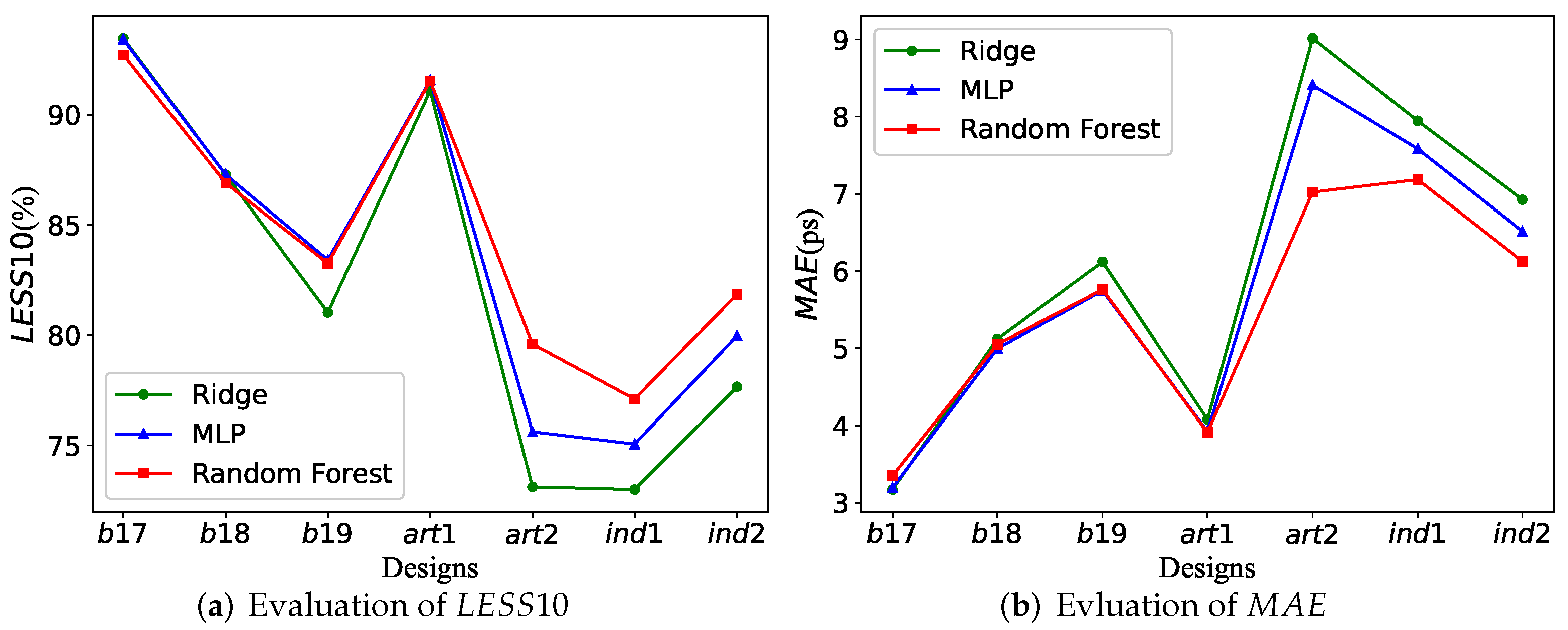
PAF can help designers to make a trade-off between acceleration effect and prediction accuracy, and to select the most suitable combination. Incidentally, the accuracy evaluation criterion is customizable, which allows our algorithm to be adapted to different goals.
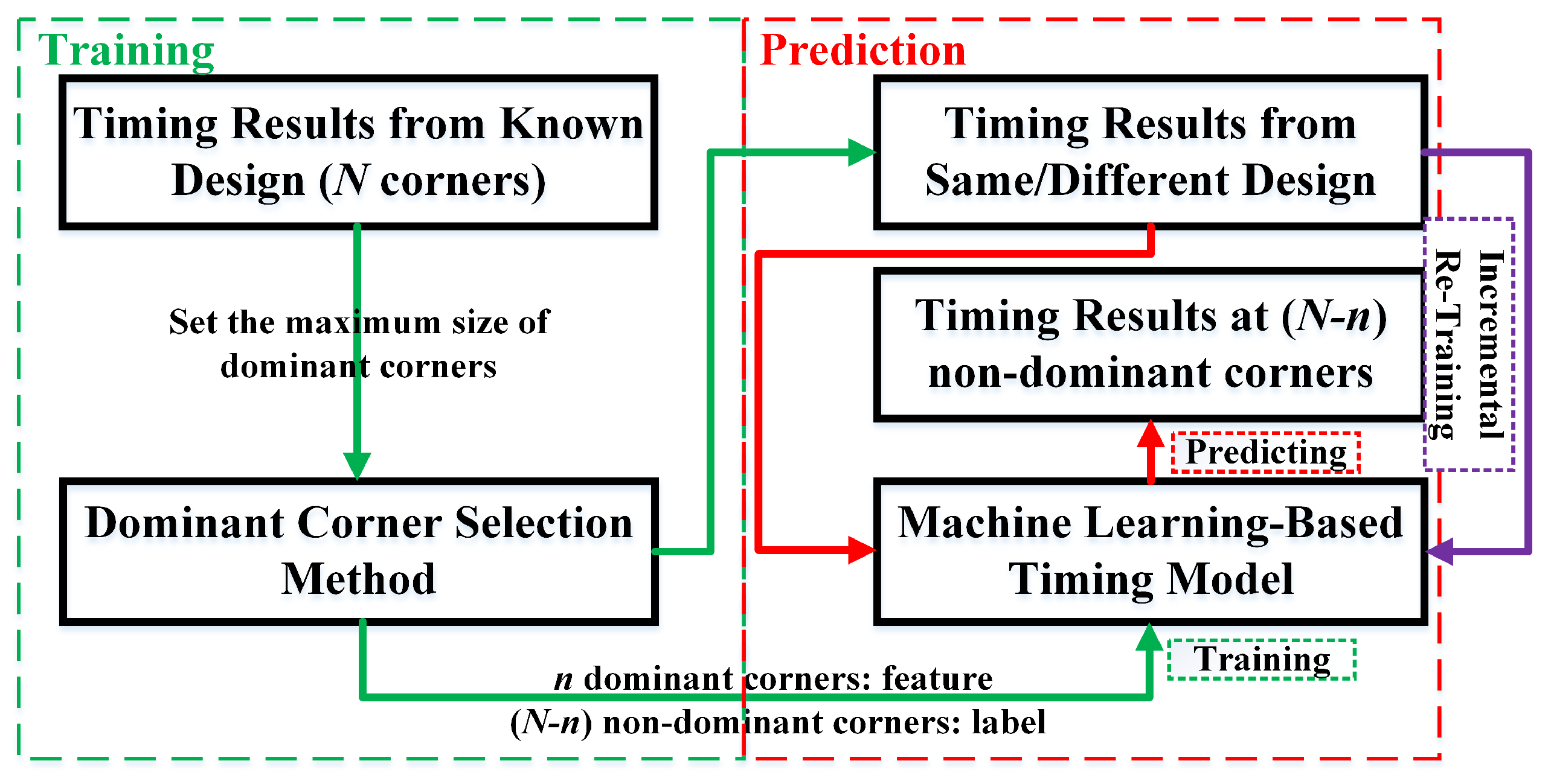
4.1.2. An Application Flow of Multi-Corner Timing Prediction
In this section, we establish an application flow of our multi-corner timing prediction, which is shown in
Figure 5.
Training: Timing results of a few paths at N corners are obtained to find the best dominant corner combination. According to the PAF generated by our dominant corner selection algorithm, we choose the combination of size n. After that, the timings at n dominant corners and non-dominant corners are used as features and labels to train the timing model.
Prediction: The trained timing model can be used to predict the timing of the same design or different designs, as long as these designs use the same chip manufacturing process. Before making the prediction, the timing of large paths at n dominant corners needs to be obtained by the STA tool. Then, the timing at the remaining non-dominant corners can be predicted.
Incremental Re-Training: Generally speaking, the more training data, the better the performance of the model. In order to continuously improve the generalization of the timing prediction model, an incremental training mechanism is integrated into this flow. That is to say, the model is re-trained by the newly obtained timing results at N corners.


